| Issue |
A&A
Volume 650, June 2021
|
|
|---|---|---|
| Article Number | A36 | |
| Number of page(s) | 13 | |
| Section | Interstellar and circumstellar matter | |
| DOI | https://doi.org/10.1051/0004-6361/202039836 | |
| Published online | 02 June 2021 | |
Simulating observable structures due to a perturbed interstellar medium in front of astrospheric bow shocks in 3D MHD
1
Ruhr-Universität Bochum, Fakultät für Physik und Astronomie, Institut für Theoretische Physik IV,
44780
Bochum,
Germany
e-mail: This email address is being protected from spambots. You need JavaScript enabled to view it.
2
Ruhr-Universität Bochum, Research Department,
Plasmas with Complex Interactions,
44780
Bochum,
Germany
3
Ruhr Astroparticle and Plasma Physics (RAPP) Center,
44780
Bochum,
Germany
4
Ruhr-Universität Bochum, Fakultät für Physik und Astronomie, Astronomisches Institut,
44780
Bochum,
Germany
Received:
3
November
2020
Accepted:
26
March
2021
Abstract
Context. While the shapes of many observed bow shocks can be reproduced by simple astrosphere models, more elaborate approaches have recently been used to explain differing observable structures.
Aims. By placing perturbations of an otherwise homogeneous interstellar medium in front of the astrospheric bow shock of the runaway blue supergiant λ Cephei, the observable structure of the model astrosphere is significantly altered, providing insight into the origin of perturbed bow shock images.
Methods. Three-dimensional single-fluid magnetohydrodynamic (MHD) models of stationary astrospheres were subjected to various types of perturbations and simulated until stationarity was reached again. As examples, simple perturbations of the available MHD parameters (number density, bulk velocity, temperature, and magnetic field) as well as a more complex perturbation were chosen. Synthetic observations were generated by line-of-sight integration of the model data, producing Hα, 70 μm dust emission, and bremsstrahlung maps of the perturbed astrosphere’s evolution.
Results. The resulting shock structures and observational images differ strongly depending on the type of the injected perturbation and the viewing angles, forming arc-like protrusions or bifurcations of the bow shock structure, as well as rings, arcs, and irregular structures detached from the bow shock.
Key words: stars: winds, outflows / magnetohydrodynamics (MHD) / shock waves
© ESO 2021
1 Introduction
Three-dimensional (3D) magnetohydrodynamics (MHD) have recently come into focus as a viable tool for further examining and understanding the structures of astrospheres (e.g. Katushkina et al. 2018; Gvaramadze et al. 2018; Scherer et al. 2020). By changing these models’ orientations with respect to an observer’s line of sight (LOS), the generation of synthetic observations produces images similar to genuine data of actual bow shocks (BSs; e.g. Meyer et al. 2017; Katushkina et al. 2018; Baalmann et al. 2020). However, the shapes of many BSs (see e.g. Kobulnicky et al. 2016) look decidedly dissimilar to those created by the above approach. By introducing inhomogeneities and perturbations to the interstellar medium (ISM; cf. e.g. Borrmann & Fichtner 2005), further observations of BSs can be reproduced on a case-by-case basis (e.g. Gvaramadze et al. 2018).
However, because of the variety of possible perturbations (see Sects. 2.3 and 2.4) and the lack of observational data that could constrain them, this approach requires a great deal of effort and insight for each observational image that is to be reproduced. To facilitate this process, the influence of different perturbations on a model astrosphere’s structure must be understood. As a first step, in this paper simple inhomogeneities of all available MHD quantities are placed in the ISM in front of the model’s BS; a more complex perturbation is examined as well. While the simple inhomogeneities (see Sect. 3.1) are motivated by computational reasons, resulting in increases in the number density, temperature, bulk speed, or magnetic field by a factor of ten, the characteristics of the complex perturbation (see Sect. 3.2) correspond to those common for tiny scale atomic structures (TSASs) and tiny scale ionised structures (TSISs; cf. Stanimirović & Zweibel 2018 and references therein).
Because a significant number of ISM perturbations are the cause of (M)HD shocks, investigations into colliding shocks (Courant & Friedrichs 1948) are also of interest to this examination (see e.g. Fogerty et al. 2017). While these studies are generalisable and applicable to various MHD scenarios, their origin lies outside the scenario of astrospheres, instead focusing on, for example, coronal mass ejections (e.g. Lugaz et al. 2005), interplanetary magnetic clouds (Xiong et al. 2009), or colliding winds of binary systems (Kissmann et al. 2016).
Within the scope of this work, λ Cephei is used as a prototype star to generate a large-scale astrosphere. As a runaway blue supergiant of spectral type O6.5, λ Cephei features a high velocity relative to a dense ISM as well as a strong stellar wind (SW), resulting in a BS distance on the scale of several parsecs. The simulated structures are examined via contour plots of the MHD values and by generating synthetic sky maps in Hα, in 70 μm dust emission, and, for selected cases, in bremsstrahlung.
An overview of the methodology used for simulating and examining the model astrospheres is given in Sect. 2. The results are presented in Sect. 3 and compared to the classification of wind-ISM interactions by Cox et al. (2012) in Sect. 4. Conclusions are drawn in Sect. 5.
2 Methodology
A brief overview of the computational model is given in Sect. 2.1, followed by details of the perturbations’ computation (Sect. 2.2), shapes (Sect. 2.3), and types (Sect. 2.4). The methodology for analysing the simulations, including synthetic observations, is presented in Sect. 2.5 and applied to the unperturbed models in Sect. 2.6. Numerical diffusion as the expected main source of errors is examined in Sect. 2.7.
2.1 Computational model
To model the astrosphere in 3D single-fluid MHD, the semi-discrete finite-volume CRONOS code (Kissmann et al. 2018) was used, solving the equations of ideal MHD,
 (1)
(1)
 (2)
(2)
![Mathematical equation: \begin{equation*} \frac{\partial e}{\partial t} + \nabla \cdot \left[ \left(e + p + \frac{1}{2\mu_0} \left| \vec{B} \right|^2 \right) \vec{u} - \frac{1}{\mu_0}\left(\vec{u} \cdot \vec{B} \right) \vec{B}\right] = 0,\end{equation*}](/articles/aa/full_html/2021/06/aa39836-20/aa39836-20-eq3.png) (3)
(3)
 (4)
(4)
with an HLL Riemann solver and a second-order Runge-Kutta scheme, where: n, u, p, B, and e are the number density, fluid velocity, thermal pressure, magnetic induction, and total energy density, respectively; m and μ0 are the proton mass and the vacuum permeability, and ⊗ represents the dyadic product. The system was closed by the additional equations
 (5)
(5)
 (6)
(6)
where γ = 5∕3 is the polytropic index of a mono-atomic ideal gas. For examining the model, the temperature T = p∕(2nkB) was evaluated instead of the thermal pressure, assuming an ideal gas with an additional factor 1∕2 from the assumption of thermodynamic equilibrium between electrons and protons (p = pe + pp = 2pp), where kB is the Boltzmann constant. Internally, however, CRONOS uses the thermal energy density eth = p∕(γ − 1) instead of the temperature T, which is reflected by the physical parameters available for the later perturbations.
To allow for heating processes, the term
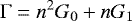 (7)
(7)
was added to the right-hand side of Eq. (3) as described in Kosiński & Hanasz (2006), following Reynolds et al. (1999). Here, G0 =1 × 10⁻²⁴ erg cm3 s−1 accounts for photoionisation heating, and G1 = 1 × 10⁻²⁵ erg s−1 accounts for photoelectric heating by dust, Coulomb collisions with cosmic rays, and the dissipation of interstellar turbulence. Because n ≫ 0.1 cm−3 outside the astropause (AP; cf. Sect. 2.6), the term nG1 is negligible there. As with the heating, a cooling term following Schure et al. (2009) was used to incorporate radiative cooling for temperatures T ∈ [103.8, 108.16] K. For T < 104 K, no cooling was implemented. For T ≥ 108.16 K, the cooling value for T = 108.16 K was used; however, no such temperatures occurred in any of the models.
The computational grid was arranged in spherical coordinates (r, ϑ, φ), producing a spherical polyhedron with equidistant intervals in the radius r and equiangular intervals in the polar and azimuthal angles, ϑ and φ. While the entirety of the angular ranges ϑ ∈ [−90°, 90°] and φ ∈ [−180°, 180°] were covered by the grid, the radial range r ∈ [rSW, rISM], rSW > 0 excluded the central volume of the star and its surroundings. The number of grid cells, Nr,ϑ,φ, in each coordinate direction and the associated cell sizes, Δ(r, ϑ, φ), of the model were changed for different purposes, as displayed in Table 1, corresponding to a low-resolution but high-performance grid (lores) and a high-resolution but low-performance one (hires) for more detailed examinations. A third grid with a more similar resolution in r and ϑ, φ (eqres) was used as a reference for the examination of numerical diffusion (cf. Sect. 2.7).
The astrospheres of different stars can be simulated by choosing different boundary conditions of the modelling equations for the inner and outer edges of the grid (at r = rSW,ISM), corresponding to the spherical SW and the ISM boundary. In this paper, λ Cephei is used as an example of a particularly strong ISM inflow and SW (cf. Baalmann et al. 2020); the corresponding boundary conditions are summarised in Table 2. The ISM was assumed to be homogeneous with an oblique magnetic field orientated with respective angles ϑB and φB. By setting the angles of the ISM fluid inflow to ϑu = 90° and φu = 180°, the simulation’s x-axis was aligned with the stellar motion (i.e. the upwind direction). Accordingly, the negative x-axis points in the downwind or tail direction. The SW was set up as a spherically symmetric outflow with only a radial component, its magnetic field following Parker’s spiral (Parker 1958). For both the SW and the ISM, n and T were fixed at the respective boundaries, rSW and rISM. More detailsabout the simulation setup are presented in Scherer et al. (2016).
Simulation sizes and resolutions of the various models.
Boundary values chosen for the model of λ Cephei.
Perturbation values.
2.2 Computation of perturbations
Once the CRONOS run reached stationarity, perturbations were injected into the ISM by externally changing the parameter values of pre-selected cells. The modified simulation file was then used as the initial set of values for a new CRONOS run, either computed until the perturbed model reached stationarity again or until another custom condition was satisfied.
Because the model of λ Cephei is rotationally symmetric about its inflow axis to a reasonable degree (Baalmann et al. 2020), the axis parallel to the homogeneous ISM inflow that passes through the star, examining its ecliptic plane (cf. Sect. 2.6), is a useful approach for understanding the entire 3D structure. Therefore, all injected perturbations were centred in the ecliptic plane (ϑ = 0°).
2.3 Shapes of perturbations
Two basic shapes were chosen as the domain in which the ISM was to be perturbed: boxes and spheres. The box represents the small-scale limiting case of any shape on a finite, rectangular grid. Because the grid is spherical and not Cartesian, a box with coordinate lengths (Nr,1, Nϑ,1, Nφ,1) is not strictly cuboid but slightly trapezoid, its volume and shape depending on the coordinates (r1, ϑ1, φ1) at which it is placed. As a small-scale limiting case, Nϑ,1 = Nφ,1 = 1 was used for all box-shaped perturbations, corresponding to angular extents of  for the low-resolution models (cf. Table 1), and Nr,1 was varied to gain different shapes (cf. Table 3). For spherical perturbations, all model cells within a radius R1 around the perturbation’s centre (r1, ϑ1, φ1) were set to the perturbed values.
2.4 Types of perturbations
Inside the perturbation area, the available physical parameters of the number density n, the thermal energy density eth, the bulk velocity u, and the magnetic flux density B were set to their perturbed values. However, not all perturbations are useful for physical modelling. From a physical standpoint, injecting a perturbation at an arbitrary position inside the homogeneous ISM necessitates it either being stable enough to have moved to that position or having been generated there. For example, a perturbation of the thermal energy density eth without any further changes to n, u, or B would thus correspond to a perturbation of the temperature T that would dissolve after a short amount of time. A perturbation of the magnetic field B must be divergence-free yet would generally still dissolve without any accompanying changes to other parameters due to magnetic pressure.
A change to the bulk velocity u might naively be assumed to correspond to a clump of material moving at a different velocity through the ISM. However, because of the single-fluid approach, the entire content of a model cell would move with this new velocity, causing an immediate accumulation of material in front of as well as a cavity behind the perturbed area, in regards to the moving direction. Also, velocities must firmly lie in the non-relativistic regime because relativistic processes are not yet supported for the simulation.
Mathematically, a perturbation would remain stable if it did not change the MHD Eqs. (1)–(4) from the unperturbed case. In HD, this is true for any perturbation of the number density n because it only functions as a scaling parameter. However, in MHD, the magnetic field in Eqs. (2) and (3) generally rules this out. For a weak magnetic field (i.e. if the magnetic pressure is much lower than the thermal pressure), a perturbation in n is still reasonably stable.
The MHD equations would likely allow for other stable configurations as well. However, finding these configurations was not part of this investigation. Instead, if a perturbation was found to be unstable, it was assumed to be generated in situ, for example by turbulence.
2.5 Model analysis
The models were examined via contour plots, commonly in the ecliptic plane, via synthetic observations as described in Baalmann et al. (2020), and via viewing their 3D structure. While the last approach gives an overview of the entire model, it is insufficient for properly quantifying the results, making the other methods necessary.
For comparisons with observational images, synthetic observations of the various models are indispensable. Synthetic sky maps were created by shifting and rotating the model to the desired position and orientation and then dividing the covered area of the virtual sky into pixels on a two-dimensional (2D) grid. By calculating the emission of each model cell and their respective flux densities through the pixels, the models were projected. However, because taking the full geometry of every model cell into account would require an unreasonable amount of computing power, only the positions of each model cell’s centre were regarded when dividing the projection into the 2D grid. Thus, model cells that would be large enough to appear in two or more pixels were only counted for the pixel in which their centres were located. Because of the large number of model cells, it was assumed that the effects of multiple model cells would roughly cancel out; the resulting errors are therefore insignificant (cf. Baalmann et al. 2020). The resolution of the 2D pixel grid is dependent on the largest distance of next-neighbour cells in the 3D model and is thus limited by the angular resolution of the model. To improve the 2D pixel resolution, the 3D model was linearly interpolated with a factor of four in the radial directions before generating synthetic sky maps. This does, however, introduce visible artefacts with the lores grid that do not correspond to physical structures, for example a ring of higher flux density with a radius of 0.2° around the model centre and sharp jags perpendicular to the radial direction at the BS (cf. Sect. 2.6). Depending on the geometry, Moiré patterns typical for two overlaying grids are visible (cf. Sect. 4).
The primary observable calculated with this approach was the Hα flux,
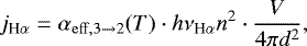 (8)
(8)
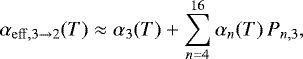
where V and d are the volume and distance to the observer of the respective model cell, h is the Planck constant, νHα = 456.81 THz is the Hα frequency, and αeff,3→2 is the temperature-dependent effective recombination rate coefficient, calculated via
 (9)
(9)
with αi(T) the temperature-dependent recombination rate coefficient of state i, and Pi,k the branching ratio from state i through state k. The αi (T) were taken from Mao & Kaastra (2016) and the Pi,k computed as in Baalmann et al. (2020) with data from Wiese & Fuhr (2009). The resulting curve for the effective recombination rate coefficient is valid for temperatures T ∈ [101, 108] K and decreases strictly monotonously from αeff,3→2(101 K) ≈ 3.6 × 10⁻¹² cm3 s−1 to αeff,3→2(108 K) ≈ 1.1 × 10⁻¹⁸ cm3 s−1.
All models were also analysed in the spectral emission due to dust at a wavelength of 70 μm. The requisite spectral emissivity εν is plotted in Fig. 1 as a function of the dimensionless radiation field U, reproduced following Henney & Arthur (2019b), where a variety of models were computed for the spectral energy distribution of an OB star using the photoionisation code Cloudy (e.g. Ferland et al. 2017). At low U, the emissivity was extrapolated with data from Draine & Li (2007), adapted by Henney & Arthur (2019b). The dimensionless radiation field U = Lλ Cep∕(4πr2cuMMP83) depends only on the distance r from the star; Lλ Cep = 6.3 × 10⁵L⊙ = 2.424 × 1039 erg s−1 is the stellar luminosity of λ Cephei, c the speed of light, and uMMP83 = 0.0217 erg s−1 cm−2∕c the energy density of the interstellar radiation field for wavelengths λ < 8 μm in the solar neighbourhood (Mathis et al. 1983; Henney & Arthur 2019b). The thus calculated spectral emissivity εν is the emitted spectral power per hydrogen atom and unit solid angle. The spectral flux for dust emission was calculated by
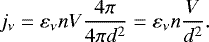 (10)
(10)
This approach is only valid under the assumption that the distribution of gas, or more specifically of ionised hydrogen, can be used as a tracer for the distribution of dust. In general, one must allow for the partial decoupling of gas and dust (Katushkina & Izmodenov 2019). However, for BSs around luminous blue supergiants with an extent of multiple parsecs, decoupling does not occur (Henney & Arthur 2019a).
For select models, the thermal bremsstrahlung flux,
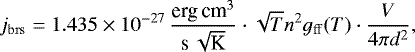 (11)
(11)
was calculated as well, with gff(T) the temperature-dependent Gaunt factor for free-free transitions (Rybicki & Lightman 1979). The Gaunt factor was calculated following van Hoof et al. (2014) and resulted in values gff (T) ∈ [1.0, 1.5[, so the usual approximation ḡ = 1.2 holds (cf. Baalmann et al. 2020). The jbrs is the flux over the entire electromagnetic spectrum without any modulation by, for example, (self-)absorption. As a simple approximation, the bremsstrahlung spectrum can be assumed to be flat up to a critical frequency,
 (12)
(12)
where v is the thermal electron speed of the respective model cell and me is the electron mass (Longair 1992). The exact spectral flux follows as
 (13)
(13)
with the spectral emissivity (Rybicki & Lightman 1979):
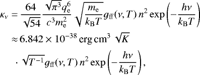 (14)
(14)
where qe, ε0, c, and kB are the elementary charge, electric constant, speed of light, and Boltzmann constant, ν is the frequency, and gff(ν, T) is the frequency- and temperature-dependent Gaunt factor taken from van Hoof et al. (2014). Absorption was incorporated by
 (15)
(15)
where the term dχν describes the fraction of radiation absorbed by a homogeneous medium between source and observer at distance d; negative values of  were set to 0. The absorption coefficient χν, calculated following Longair (1992) via
![Mathematical equation: \begin{equation*} \chi_{\nu}=\frac{\kappa_{\nu} c^2}{8\pi h\nu^3}\cdot\left[\exp\left(\frac{h\nu}{k_{\mathrm{B}}T_{\mathrm{ISM}}}\right) -1\right], \end{equation*}](/articles/aa/full_html/2021/06/aa39836-20/aa39836-20-eq18.png) (16)
(16)
was assumed to be constant from the respective model cell to the observer within a homogeneous ISM with temperature TISM. The resulting spectra for the lores grid’s final time step (cf. Sect. 2.6), both with and without modulation by absorption, are presented in Fig. 2. While the spectrum is not flat, it does remain in the same order of magnitude up to a frequency of roughly log(νcrit [Hz]) ≈ 14.5.
Equations (8) and (11) give the fluxes of the respective model cells; summation over all model cells that appear inside a pixel gives the total flux of that pixel. However, because the different resolutions of the lores and hires models lead to different 2D grid resolutions, the total fluxes at different grid resolutions of otherwise identical models differ by the ratio of the respective pixels’ solid angles. To be able to compare models of different 2D grids, the respective flux densities were obtained by dividing the fluxes as calculated by Eqs. (8) and (11) by the respective pixels’ solid angles: 5.07 × 10⁻⁸ sr for the lores grid and 1.00 × 10⁻⁸ sr for the hires grid.
 |
Fig. 1 Spectral emissivity of dust at 70 μm as a functionof the dimensionless radiation field, U = Lλ Cep∕(4πr2k), reproduced following Henney & Arthur (2019b). |
 |
Fig. 2 Bremsstrahlung spectrum of the lores grid’s final time step, unmodulated (dashed blue curve) and modulated by a homogeneous ISM between the model and the observer with T = TISM (solid red curve). Spectral domains of microwaves, far infrared (FIR), infrared (IR), ultraviolet (UV), soft X-ray (SX), and hard X-ray (HX) are delimited by vertical lines; the shaded area corresponds to the optical. |
2.6 Unperturbed models
Contour plots of the lores and the hires grids’ final time steps in the respective ecliptic plane are presented inFig. 3. The difference in the tail direction (downwards from the centre) is due to the different times of the models. The lores model (left) has reached complete stationarity at 408 kyr, whereas thehires model (right) is not yet fully stationary in the tail direction at 262 kyr.
In the contour plots of the models’ ecliptic plane, displayed in the upper row of Fig. 3, the star is located at the centre of each image, though it and its surrounding circular area with radius rSW = 0.05 pc are not included in the model. The homogeneous ISM inflow comes from the topside of the image; this is the topmost domain in both models of n= 11 cm−3, bordered at the bottom by the BS. Moving away from the star, the area with steadily decreasing density is the unperturbed SW, bordered at the top and sides by the termination shock (TS) and at the bottom by the Mach disk (MD). The area of higher densities compared tothe homogeneous ISM, situated below the BS, is the outer astrosheath, while the area of higher densities compared to the SW’s outer edge outside the TS and MD is the inner astrosheath. The inner and outer astrosheaths touch at the arc with n ≈1 cm−3, which is theAP, separating stellar from interstellar material. Along the inflow axis, the TS is located at rTS = 0.86 pc, the AP at rAP= 1.23 pc, and the BS at rBS = 1.73 pc, measured for the hires model. For the lores model, these distances are slightly shifted outwards, to 0.87, 1.25, and 1.84 pc, respectively. The MDs are located at rMD = 1.80 pc (hires) and1.81 pc (lores). The centre and the bottom row of Fig. 3 display synthetic face-on observations of the same planes for the models at a distance of 617 pc in Hα (centre row) and in dust emission (bottom row). As described in Baalmann et al. (2020), the largest part of the Hα emission comes from the outer astrosheath, resulting in the arc shape typically identified as the BS. Because the dust emission depends on the distance from the star in addition to the number density, the region of the outer astrosheath close to the AP near the inflow axis is brighter in dust emission than the regions farther from the star. This is in agreement with the results of Katushkina et al. (2018), where dust was kinetically modelled. The ring of high flux densities in both radiation types with a radius of 0.2° around the model centre and the jags perpendicular to the radial direction at the BS are artefacts introduced by the interpolation (cf. Sect. 2.5).
 |
Fig. 3 Stationary state of the unperturbed astrosphere. Top row: contour plots of log (n[cm−3]) for the final time steps of the lores (left) and hires (right) grids in the ecliptic plane (distances in pc); the cornered structure reflects the model cells. Centre row: synthetic face-on observations of the respective planes in Hα [erg cm−2 s−1 sr−1]. Bottom row:synthetic observations in infrared dust emission at 70 μm, [Jy sr−1 ] (angular extent in degrees). At a distance of 617 pc, 1° corresponds to 10.8 pc. The solid angles per pixel are 5.07 × 10⁻⁸ sr (lores) and 1.00 × 10⁻⁸ sr (hires). |
2.7 Numerical diffusion
Because of the comparatively coarse resolution in ϑ and φ, numerical diffusion is expected to play a significant role and must be taken into account while examining the calculations. To this effect, a homogeneous and non-moving ISM (u =0, B =0) on the different grids was used with a boxy perturbation in the number density (n1 = 10n0) of Nr,1 × Nϑ,1 × Nφ,1 = 50 × 1 × 1 cells (lores) and Nr,1 × Nϑ,1 × Nφ,1 = 90 × 2 × 2 cells (hires) in size. As a reference, a third grid (eqres) with a higher angular but lower radial resolution was examined as well; here the perturbation was Nr,1 × Nϑ,1 × Nφ,1 = 30 × 4 × 4 cells in size. The perturbations were injected in the ecliptic plane close to the outer boundary of the model, centred at 4.65 pc (lores), 4.61 pc (hires), and 4.74 pc (eqres), respectively.
Number density profiles of the progressing simulations are plotted in Fig. 4. As can be seen, numerical diffusion smoothed the initially sharp profile of the perturbation even after short times. While this effect is negligible in the radial direction forthe lores grid due to the high resolution, its magnitude in the angular directions is much graver. After  , the number density at the perturbation’s original position had decreased from the initial n1 = 10.0n0 to n(φ0) = 6.4n0, while the neighbouring angular cells’ number density had increased to n(φ1) = 1.7n0. As time progressed, the perturbation’s number density further decreased at its original position, while its angular extent increased. After
  , the numberdensity at the perturbation’s original position had decreased to n(φ0) = 3.2n0 and increased in its flanks to n(φ1) = 1.9n0 and n(φ2) = 1.1n0. Farther out, the number density had slightly increased: n(φ3) = 1.02n0 and n(φ4) = 1.002n0. Taking only the broadening to φ2 = 12° into account, for the lores grid this corresponds at r = 4.65 pc to a growth froma diameter of 0.5 pc to 2.3 pc perpendicular to the radial direction.
The primary reason for the intensity of the angular numerical diffusion is the confinement of the perturbation to a single angular cell (Nϑ,1 = Nφ,1 = 1 cell). Whereas the radial numerical diffusion could smooth the perturbation’s vertical flank to Gaussian-like wings while leaving the horizontal plateau untouched, the singular extent in the radial directions offered no such possibility. For a perturbation extending over a larger number of cells in the angular directions (realised by increasing either the physical size or the resolution), the angular numerical diffusion does not decrease the value of the perturbation’s horizontal plateau as much. However, increasing the number of angular cells covered by the perturbation by only a small factor does not significantly lower angular numerical diffusion, as can be seen with the hires model (centre panel in Fig. 4). Here, the perturbation covers roughly the same physical region, which means double the angular cells due to the finer angular resolution. Because a plateau spanning two cells still offers no possibility of keeping the plateau intact while smoothing its wings, the number density profiles of the hires grid barely differ from those of the lores grid. Improving the angular resolution by another factor of two, as is the case on the eqres grid, finally yields significantly different results. Here, the initial plateau covered four angular cells, marked as offsets φ0 and φ1 in Fig. 4. While the number density in the initially unperturbed cells increases more strongly compared to the previously examined grids (compare eqres φ2 to hires φ1), the outer edge of the plateau (eqres φ1, hires φ0) decreases more slowly, and the inner plateau (eqres φ0) even more slowly. However, the radial numerical diffusion on the eqres grid must be taken note of.
Because the impact of numerical diffusion decreases not only with finer angular resolutions but also with larger perturbations, the significance of numerical diffusion diminishes for spread-out perturbations such as v5blb (cf. Sect. 3.1), especially if computed on the hires grid like b4blb (cf. Sect. 3.1) and n2blb (cf. Sect. 3.2). While a finer angular resolution would be preferable, the simulation’s runtime unfortunately increases with approximately the fourth power of the angular number of cells: Keeping the two angular resolutions equal (Δφ = Δϑ) already amounts to a square increase in the number of computational cells; furthermore, the number of time steps per physical time is, to a reasonable approximation, proportional to the number of angular cells as well. This is because the length of a time step δt is limited by the cell with the smallest value of δtcell = CCFLΔL∕cmax, where ΔL is the spatial cell length, cmax is the largest characteristic speed, and CCFL comes from the Courant-Friedrichs-Lewy condition (see Kissmann et al. 2018); the last two values can be assumed as constant for the purpose of setting the grid’s resolution. Because ΔL = min{Δr, rSWn2(Δϑ)∕2} and rSW n2(Δϑ)∕2 = 0.025Δr for the hires grid, improving the angular resolution sharply decreases δt as well. Thus, doubling the angular resolution necessitates an increase in computational resources by nearly a factor of 16. Even when the total number of cells is kept constant by impairing the radial resolution, as was done from hires to eqres, the computational cost still increases with the square of the factor of angular refinement.
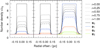 |
Fig. 4 Number density profiles of the diffusion test for the lores (left), hires (centre), and eqres (right) grids; the number density is scaled by the unperturbed ISM value. Dash types denote the time since injection in 44 828 kyr, and line colours denote the offset in the φ-direction, with φi= φ0 + i Δφ. |
3 Results
An overview over the computed perturbations is given in Table 3. Simple perturbations of a single physical variable (number density, temperature, velocity, or magnetic field) are examined in Sect. 3.1, and larger and more complex perturbations are examined in Sect. 3.2.
3.1 Simple perturbations
The nblob model describes a spatially small perturbation of the ISM, increasing the number density by a factor of ten to n1 = 110 cm−3 inside a volume of Nr,1 × Nϑ,1 × Nφ,1 = 30 × 1 × 1 cells, injected close to the outer edge of the model (![Mathematical equation: $r_1\in[1062, 1091]\,\textrm{cells}\ \hat{\approx}\ [4.61, 4.79]\,\textrm{pc}$](/articles/aa/full_html/2021/06/aa39836-20/aa39836-20-eq21.png) ) along the inflow axis. In physical terms, the volume of this pyramid frustum is V1 =
) along the inflow axis. In physical terms, the volume of this pyramid frustum is V1 =  , an excess of V1 (n1 − n0) ≈ 9.05 × 1055 protons and electrons, and an excess mass of 0.0761M⊙. All other simulation values (eth, u, B) remained constant; from T ∝ eth∕n, it follows that T1 = T0∕10 = 900 K. At this temperature, cooling holds little significance, but heating increases the energy density, according to Eq. (7), by Γ ≈n1G0 ≈ 1.21 × 10⁻²⁰ erg cm−3 s−1. Typically, the timescale of heating τΓ is approximated by dividing the increase in thermal energy by the heating power, in this case τΓ = eth∕Γ ≈ 3kB(T0 − T1)∕(n1G0) = 966.5 yrs. However, heating is incorporated into the model as a source term in Eq. (3). Thus, heating does not directly increase the thermal energy density but rather the total energy density, which is dominated by the kinetic energy density (i.e. the ram pressure): Within the perturbation right after its injection, the kinetic energy density amounts to
  (99.2% of the total energy density), the magnetic energy density to |BISM|2∕(2μ0) ≈ 3.98 × 10⁻¹² erg cm−3 (0.1%), and the thermal energy density to 3n1kBT1 ≈ 4.10 × 10⁻¹¹ erg cm−3 (0.7%). Over a time span of Δt = 4.4828 kyr, the heating term results in an increase in the energy density by 1.71 × 10⁻⁹ erg cm−3, which is 29.0% of the total energy density at injection. This additional energy does not remain inside the model cells or the perturbation region, and the heating term changes all MHD quantities to values different from their non-heated counterparts. While the perturbed region does heat up to 1347.512 K after Δt = 4.4828 kyr, only 0.053 K of this increase is due to the additional heating term, the rest stemming from pure MHD and numerical effects. Thus, the energy source term typically identified as ‘heating’ actually causes only a negligible amount of heating but is nevertheless significant for the evolution of total energy within the perturbation. Furthermore, this implies in particular that the often used approximation for the heating timescale does not hold since it neglects the self-consistent conversion of thermal into other forms of energy.
Cross-sections of the model’s ecliptic at selected times are displayed in Fig. 5 (top row), with corresponding synthetic observations in Hα shown in the bottom row of the same figure. Directly after injection (leftmost column of panels in Fig. 5, Δt = 0 kyr), the perturbation distends to a Gaussian shape due to numerical diffusion (cf. Sect. 2.7) and slowly widens further (centre-left column, Δt = 7 × 4.4828 kyr) until it impacts the BS. It enhances the number density within a small region inside the outer astrosheath by roughly a factor of two (centre-right column, Δt = 9 × 4.4828 kyr) before dispersing inside the outer astrosheath (rightmost column, Δt = 12 × 4.4828 kyr). The collision of perturbation and outer astrosheath causes a small indentation in the BS around the centre of impact (cf. centre-right column) that takes roughly 10 kyr to fill out.
While the perturbation is well visible in Hα when still inside the homogeneous ISM, contrasting by roughly a factor of two even when partially dissolved (centre-left column), neither the enhanced density of the outer astrosheath after the impact nor the dent in the BS are readily apparent (centre-right column). This is in part due to the low resolution of the model but mostly stems from the poor contrast between the perturbation and the outer astrosheath shortly before the impact. A perturbation of higher density or larger size would cause a more notable indentation, both in size and density enhancement (cf. the n2blb model in Sect. 3.2).
Because dust emission is dependent on the distance to the star, the perturbation is nearly invisible at the time of injection (left column) and only faintly visible before impacting the BS (centre-left column). Because the post-impact density enhancement occurs at the BS surface of the outer astrosheath, where dust emission is weaker due to the larger distance from the star compared to the AP surface, the small density perturbation is of little significance for the observable dust.
The t1blb model similarly describes a small perturbation that increased the temperature from TISM = 9 kK to T1 = 90 kK inside a volume of Nr,1 × Nϑ,1 × Nφ,1 = 50 × 1 × 1 cells, injected 300 cells in front of the BS (r1 ∈ [712, 761] cells) along the model’s inflow axis. In physical units, the perturbation’s centre is located 1.41 pc in front of the BS, with a radial thickness of 0.22 pc and an average width of 0.33 pc. This perturbation decreases its number density immediately after injection to regain thermal pressure equilibrium and disperses shortly afterwards, not causing any notable change in the astrosphere’s structure or synthetic observations.
The same does not hold true for a similar perturbation of the velocity. In the v5blb model (cf. Fig. 6), the shape of theperturbation was set up in the same way as for the t1blb model but the speed was increased from uISM = 80 km s−1 to u1 = 800 km s−1, keeping the velocity’s orientation (leftmost column). As expected, the perturbation distends quickly, causing a cavity at the perturbation’s co-moving position as well as an accumulation of material in front of and, to a lesser degree, behind it (centre-left column, Δt = 1 × 4.4828 kyr). The cavity significantly distorts the shape of the outer astrosheath upon impacting the BS (centre column, Δt = 2.5 × 4.4828 kyr), at first decreasing its density along the inflow axis (centre-right column, Δt = 4 × 4.4828 kyr) before generating a shell-like structure of two high-density areas separated by a low-density one (rightmost column, Δt = 6 × 4.4828 kyr). Afterwards, the shells fall together, and the configuration slowly returns to the stationary state (cf. Fig. 3, Δt ≈ 15 × 4.4828 kyr). This behaviour can be observed in the synthetic Hα flux densities as well (bottom row of Fig. 6). The formed cavity results in lower flux densities, by roughly a factor of two, bordered by a region of higher flux densities, again by roughly a factor of two. In 70 μm dust emission, the outer border of the cavity is only faintly visible due to its larger distance from the star. This is particularly prominent for the shell-like structure at Δt = 6 × 4.4828 kyr (right column), where the inner shell dominates over the outer one in dust emission but is much fainter in Hα.
The lores grid cannot resolve the magnetic structure that evolves for a similar perturbation of the magnetic field, so the hires model was used instead. The b4blb model had a perturbation of the magnetic vector potential’s ϑ-component (Aϑ= 3.5 comp. units) injected at a position and size comparable to those of the perturbations of the t1blb and v5blb models, resulting in a perturbed magnetic field B1 =B0 + ∇ × A inside a volume of Nr,1 × Nϑ,1 × Nφ,1 = 90 × 2 × 2 cells, injected 540 cells in front of the BS (r1 ∈ [1233, 1322] cells). In physical units, the perturbation’s centre was located 1.41 pc in front of the BS, with a radial thickness of 0.22 pc and an average width of 0.31 pc. The resulting magnetic field B1 formed a boxy, clockwise vortex in the (r, φ)-plane for ϑ = 0° (cf. Fig. 7): The ϑ-component of the magnetic flux density remained homogeneous, whereas the radial component increased to Br,1 (φ = −4.22°) = 8.1 nT on the ‘left’ side and to Br,1 (φ = −1.40°) = −9.0 nT on the ‘right’ side (first panel); the φ-component increased to Bφ,1(r = 3.27 pc) = 269 nT on the ‘top’ side and to Bφ,1(r = 3.24 pc) = −269 nT on the ‘bottom’ side, and also from Bφ,0 ≈ 0.3 nT to Bφ,1 ∈ [0.46, 0.49] nT ‘inside’ the vortex at r ∈ [3.24, 3.27] pc (second panel). On average, the perturbed magnetic flux density is ten times larger than the unperturbed one,  , motivating the seemingly arbitrary choice of Aϑ = 3.5 computational units. Ideally, the magnetic vortex’s outer edge would form a circle and not a trapezium; however, this requires either a finer resolution or a larger perturbation.
After injection, the perturbation forms two local minima in the number density around the top and bottom side of the vortex (cf. Fig. 8, leftmost column, Δt = 0.5 × 4.4828 kyr). Due to the higher magnetic pressure inside the perturbation, it quickly expands to form a spherical cavity with an outer wall of higher number density (centre-left column, Δt = 2.5 × 4.4828 kyr). After the impact of the perturbation with the BS, material from the outer astrosheath flows into the cavity, decreasing the number density downstream of the BS. When the perturbation’s upwind upward slope of the number density impacts the BS, it causes a front of dense material to form. The impact of the upwind part of the perturbation’s outer wall and the BS creates a second dense front, while a region of low density remains between these two fronts in a shell-like structure (centre column, Δt = 7 × 4.4828 kyr). Afterwards, the BS and AP continue to move outwards to form a bump, reaching their outermost position at Δt = 1.15 × 4.4828 kyr after injection (centre-right column). The bump slowly widens and decreases in density until it reaches its maximum extent (rightmost column, Δt = 15 × 4.4828 kyr), from which point the structure returns to its stationary state (cf. Fig. 3, Δt ≈ 25 × 4.4828 kyr). In total, the magnetic perturbation causes a behaviour similar to that of the velocity perturbation (v4blb), creating a cavity that modifies the shape of the outer astrosheath.
The synthetic observations in Hα are comparable to those of the v4blb model as well. The perturbation’s cavity before impacting the BS is visible as a very slight decrease in Hα brightness (centre-left column). After the perturbation impacts the BS, the small-scale shell-like structure is visible for a short time (centre column) but quickly smudges to a blurred distortion of the arc structure. In 70 μm dust emission, the shell-like structure’s outer shell is much fainter.
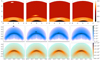 |
Fig. 5 Evolution of the nblob perturbation. Top row: cross-sections of the log number density, log (n [cm−3]), in the nblob model’s ecliptic plane at Δt ∈{0, 7, 9, 12} × 4.4828 kyr after injecting the perturbation (distances in pc). The displayed images show the (r, φ)-plane for ϑ = 0°, i.e. the ecliptic of the model. Centre row: synthetic observations of the above models in Hα [erg cm−2 s−1 sr−1] at a distanceof 617 pc, face-on to the ecliptic (angular extent in degrees). The colour scale has been truncated on both ends; values below the minimum threshold are not displayed. Bottom row: synthetic observations of the same configuration in 70 μm dust emission [Jy sr−1]. The solid angle per pixel is 5.07 × 10⁻⁸ sr. |
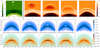 |
Fig. 6 Evolution of the v5blb perturbation. Top row: cross-sections of the v5blb model’s ecliptic plane at Δt ∈ {0, 1, 2.5, 4, 6} × 4.4828 kyr after injecting the perturbation in the absolute speed (log(u [km s−1]), left panel) and in the number density (log(n [cm−3]), four right panels; distances in pc). The white arrow in the left panel indicates the movement direction of the perturbation with respect to the surrounding ISM. Centre row: synthetic observations of the above models in Hα [erg cm−2 s−1 sr−1] at a distanceof 617 pc, face-on to the ecliptic (angular extent in degrees). The colour scale has been truncated at the bottom end; values below the minimum threshold are not displayed. Bottom row: synthetic observations of the same configuration in 70 μm dust emission [Jy sr−1]. The solid angle per pixel is 5.07 × 10⁻⁸ sr. |
 |
Fig. 7 Magnetic structure of the b4blb perturbation: r-component (left) and φ-component (right) of the magnetic flux density B for ϑ = 0° (linear scales of the magnetic flux density in nT, distances in pc). The red arrows indicate the orientation of the magnetic field. |
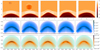 |
Fig. 8 Evolution of the b4blb perturbation. Top row: cross-sections of the log number density log (n [cm−3]) in the b4blb model’s ecliptic plane at Δt ∈{0.5, 2.5, 7, 11.5, 15} × 4.4828 kyr after injecting the perturbation (distances in pc). The navy blue arrow in the left panel indicates the direction of the magnetic vortex. Centre row: synthetic observations of the above models in Hα [erg cm−2 s−1 sr−1] at a distanceof 617 pc, face-on to the ecliptic (angular extent in degrees). The colour scale has been truncated at the bottom end; values below the minimum threshold are not displayed. Bottom row: synthetic observations of the same configuration in 70 μm dust emission [Jy sr−1]. The solid angle per pixel is 1.00 × 10⁻⁸ sr. |
3.2 Stronger perturbations
A larger perturbation was injected in the n2blb model, computed in high resolution. As in the nblob model, the perturbation’s number density was increased by an order of magnitude to n1 = 110 cm−3, while all other simulated values remained unchanged (p = const. ⇒ T1 = T0∕10). The perturbation’s shape was a sphere with a radius R1 = 225Δr ≈ 0.544 pc, injected  in front of the BS at
 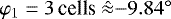 , meaning that the perturbation’s centre was y1 = (rBS + 0.725 pc)tanφ1 ≈ 0.425 pc off the inflow axis. Ecliptic cross-sections at selected times are presented in the top row of Fig. 9; the leftmost column shows the model at injection.
Moving parallel to the inflow axis, the perturbation impacts the BS off-centre and severely indents it, causing a buildup of material in the outer astrosheath by almost an order of magnitude in the number density (centre-left column, Δt = 4 × 4.4828 kyr). The perturbation continues to move parallel to the inflow axis, distorting both the AP and the TS and causing a second buildup of material (centre column, Δt = 7 × 4.4828 kyr). Both buildups move farther in the tail direction and combine (centre-right column, Δt = 9 × 4.4828 kyr). At this point in time, the perturbation is at its closest position to the star. Its momentum towards the star is overcome by the SW, which causes the inner astrosheath to extend outwards again (right column, Δt = 14 × 4.4828 kyr). As the perturbation continues to move in the tail direction, the astrosphere slowly returns to its stationary state, which is regained after about Δt = 29 × 4.4828 kyr ≈ 130 kyr.
In rows two and three of Fig. 9, synthetic observations of the Hα flux density are presented for face-on (row 2) and edge-on (row 3) orientations of the model’s ecliptic plane; the two bottom rows show the same for bremsstrahlung. In Hα, the perturbation is brighter than the outer astrosheath by roughly an order of magnitude, darkening only after the perturbation has mostly dissolved (rightmost column). The two discrete buildups of dense material corresponding to the centre column of Fig. 9 blur together into one Hα-bright clump with a distinct edge at the side towards the star, which marks the TS. A second clump of Hα-bright material, roughly 0.1 pc upwind of the first clump, is located just upwind of the BS, where the perturbation’s movement has caused the BS to bifurcate. The local maximum of Hα emission is not caused by a local maximum of the number density, which remains at n =nISM = 11 cm−3, but by a drastic decrease in the temperatureto values as low as T = 10−3 K. This clump appears to be very narrow in edge-on observations of the ecliptic (lower row), covering only a single pixel column. Both the unphysicallylow temperatures and the singular extent of this region indicate that it likely is a numerical artefact and should be dismissed for observational purposes. The movement and dissolution of the clump made of material from the perturbation are easily visible in Hα, leaving a bright trail (rightmost column) that is particularly distinctive in face-on observations (upper row).
In bremsstrahlung (rows 4 and 5 in Fig. 9), the movement of the perturbation can be clearly followed as well. While the perturbation is not as bright compared to the ISM emission in bremsstrahlung as it is in Hα at injection (leftmost column), the buildup of dense material after the perturbation impacts the BS causes said clump to emit in bremsstrahlung just as brightly as it does in Hα. The second clump, caused by low temperatures, cannot be seen in bremsstrahlung, as can be expected from Eq. (11). While the bremsstrahlung flux density is of the same order of magnitude compared to the Hα flux density, one must keep in mind that Hα is line emission, whereas bremsstrahlung is continuous, as seen in Fig. 2. Thus, the spectral bremsstrahlung flux density is far lower compared to that of Hα.
The apparent structure in 70 μm dust emission is similar to that of bremsstrahlung. The most notable difference is that the dust emission arc is hollow, as it is for Hα: because little emission comes from the inner astrosheath, the arc structure has a distinct inner edge. This is not true for bremsstrahlung, where the arc structure is filled out.
 |
Fig. 9 Evolution of the n2blb perturbation. Top row: cross-sections of the log number density log (n [cm−3]) in the n2blb model’s ecliptic plane at Δt ∈{0, 4, 7, 9, 14} × 4.4828 kyr after injecting the perturbation (distances in pc). Six bottom rows: synthetic observations of the above models in Hα (rows 2 and 3) andbremsstrahlung (rows 4 and 5) [erg cm−2 s−1 sr−1] and 70 μm dust emission [Jy sr−1] (rows 6 and 7) at the same times and at a distance of 617 pc, face-on (rows 2, 4, and 6) and edge-on (rows 3, 5, and 7) to the ecliptic (angular extent in degrees). The colour scales have been truncated at the bottom end; values below the minimum threshold are not displayed. The solid angle per pixel is 1.00 × 10⁻⁸ sr. |
 |
Fig. 10 Synthetic observations of the stationary astrosphere on the hires grid in 70 μm dust emission [Jy sr−1] at a distanceof 617 pc at different angles: with the LOS in the direction of the star’s relative motion (left), at 45° to the ecliptic’s face-on view (centre), and at 45° to the ecliptic’s edge-on view (right). The solid angle per pixel is 4.00 × 10⁻⁸ sr. |
4 Observational classification
To facilitate comparing the perturbed models to observational data, synthetic observations for additional viewing angles were generated. Figure 10 shows the unperturbed astrosphere at stationarity in the hires grid in 70 μm dust emission from three different perspectives: In the left panel, the LOS is oriented parallel to the star’s relative motion; because the astrosphere is reasonably symmetric about this axis, the resulting image shows only a slight radial gradient. The dust emission is not significantly higher compared to the homogeneous ISM. The two right panels both show the astrosphere at an inclination of 45° between the axis of stellar motion and the LOS. The centre panel displays a tilted view of the face-on ecliptic; this rotation is halfway between the zero-inclination perspective of the left panel and the face-on perspective used above (see e.g. Fig. 3). The right panel displays a tilted view of the edge-on ecliptic, halfway between the zero-inclination perspective and the edge-on perspective only used for analysing the n2blb model (rows 3, 5, and 7 of Fig. 9). Because of the astrosphere’s symmetry, the two images only differ in their geometry, most notably the Moiré patterns caused by the projection.
In Fig. 11, further rotations of the v5blb model in 70 μm dust emission are displayed. The configuration is that of Fig. 6 but rotated to the zero-inclination perspective in the top row and the 45°-inclination face-on perspective in the bottom row. Because of the rotational symmetry about the inflow axis, the 45°-inclination edge-on perspective does not significantly differ from the face-on view and is therefore not plotted. For both rows of images, the colour scales have been readjusted to utilise the full contrast. The Moiré patterns, fairly distinct at the images’ outer edges, are projection effects.
At zero inclination, the total emission is reduced by roughly three-quarters compared to the 90°-inclination perspective of Fig. 6. The perturbation is distinctly visible as a ring of high emission, similar to Class III ring-type interactions as described by Cox et al. (2012). At 45° inclination, the perturbation’s outer border is not visible as a shell-like structure as it is at 90° (Fig. 6). Instead, the ‘bow shock’ arc shows a double structure, with an inverted and much fainter arc below. For inclination angles ![Mathematical equation: $\in\left]0{^{\circ}}, 45{^{\circ}}\right[$](/articles/aa/full_html/2021/06/aa39836-20/aa39836-20-eq27.png) , the two arcswould appear more similar in intensity and more circular in shape. A denser or hotter outer border of the perturbation would further increase the intensity, resulting in an image similar to Class II eye-type interactions as described by Cox et al. (2012).
, the two arcswould appear more similar in intensity and more circular in shape. A denser or hotter outer border of the perturbation would further increase the intensity, resulting in an image similar to Class II eye-type interactions as described by Cox et al. (2012).
Further projections of the n2blb model in 70 μm dust emission are displayed in Fig. 12; the configuration is that of Fig. 9 for different rotational angles. As in Fig. 11, the first two rows are the zero-inclination and the 45°-inclination face-on ecliptic perspective. Because of the model’s asymmetry, the 45°-inclination edge-on ecliptic perspective is additionally displayed in the bottom row.
At zero inclination, only the perturbation is visible as a disk of high emission that becomes more and more distorted as the perturbation loses its spherical shape. At a time of Δt = 9 × 4.4828 kyr after injection, the former disk has lost all symmetry but remains fairly compact, akin to a Class IV irregular-type interaction as described by Cox et al. (2012). The perturbation’s shape distorts further, resulting in an arc-like shape at Δt = 14 × 4.4828 kyr after injection that looks similar to the arc-like shapes typically identified as BSs. However, following the classification of Cox et al. (2012), unlike true BSs, this structure would not be classified as a Class I fermata-type interaction because its opening angle is far below 120°. At an inclination of 45°, the perturbation’s distorted disk detaches from the outer astrosheath’s arc shortly after impact (Δt = 4 × 4.4828 kyr) and remains discrete until the two structures seemingly coalesce in the face-on perspective (Δt = 14 × 4.4828 kyr), producing a spiral-like shape. In the edge-on perspective, this does not occur; instead, the perturbation diffuses to a larger but fainter structure compared to the outer astrosheath’s distinct arc. By themselves, the perturbation’s distorted disk and the outer astrosheath’s arc would be classified as Class IV irregular-type and Class I fermata-type interactions, respectively, whereas together the arc shape prevails for the purpose of classification. However, it should be noted that the arc shapes of the 45°-inclination face-on perspective can lead to a misidentification of the star’s relative motion: By the shape of the arc alone, the star’s relative motion appears to point to the top right and the top left at Δt = 9 × 4.4828 kyr and Δt = 14 × 4.4828 kyr, respectively.
 |
Fig. 11 Synthetic observations of the v5blb model at Δt ∈{0, 1, 2.5, 4, 6} × 4.4828 kyr after injecting the perturbation in 70 μm dust emission [Jy sr−1] at a distanceof 617 pc at different angles: with the LOS in the direction of the star’s relative motion (top) and at 45° to the ecliptic’s face-on view (bottom). The solid angle per pixel is 4.00 × 10⁻⁸ sr. |
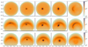 |
Fig. 12 Synthetic observations of the n2blb model at Δt ∈{0, 4, 7, 9, 14} × 4.4828 kyr after injecting the perturbation in 70 μm dust emission [Jy sr−1] at a distanceof 617 pc at different angles: with the LOS in the direction of the star’s relative motion (top), at 45° to the ecliptic’s face-on view (centre), and at 45° to the ecliptic’s edge-on view (bottom). The solid angle per pixel is 7.13 × 10⁻⁹ sr. |
5 Conclusions
Simple perturbations of the number density, the temperature (thermal pressure), the bulk velocity, and the magnetic flux density were injected in front of the model BS (cf. Sect. 3.1). While the thermal perturbation dissolved almost immediately and the density perturbation caused no significant changes to the astrosphere’s structure, both the velocity and the magnetic perturbations drastically altered the BS shape by adding abubble-like structure connected to the BS. These modified structures were visible for about 10 kyr, roughly the travel time through the perturbed domain with the ISM’s bulk speed (i.e. the speed of the star’s relative motion). A larger perturbation of the number density likewise modified the observable structure by creating a bifurcation of the BS. In all examined cases, the astrosphere returned to its previous stationary state after few tens of thousands of years, comparable to the travel time given by the astrosphere’s extent and the perturbation’s speed of motion. Depending on the orientation of the star’s relative motion with respect to the observer’s LOS, the resulting images of the perturbed astrospheres differ strongly. Using the classification by Cox et al. (2012), the above-mentioned bubble-like structures resulted in Class I fermata-type, Class II ring-type, or Class III eye-type interactions, whereas the bifurcation perturbation was visible as a Class I or a Class IV irregular-type interaction.
From a numerical standpoint, it has become clear that higher angular resolutions are preferable to reduce the uncertainty introduced by numerical diffusion. However, doubling the number of angular cells, for example, would necessitate an increase in computational resources by a factor of eight. Interpolating the model before generating synthetic observations can drastically improve the image resolution, though at the risk of introducing Moiré patterns, but it has no impact on the problem of numerical diffusion.
From the presented images, it is apparent that even simple perturbations can cause a variety of different observational shapes. More complex perturbations, as examined for example by Gvaramadze et al. (2018), would likely allow the replication of many distorted BS structures. The exact reproduction of a single object, as performed in the aforementioned study, requires high resolutions and precise insights into the respective object and its immediate surroundings, whereas this study’s aim is to provide part of that insight from multiple low-resolution simulations.
Acknowledgements
We appreciate the valuable suggestions and comments of the referee, William Henney. K.S. is grateful to the Deutsche Forschungsgemeinschaft (DFG), funding the project SCHE334/9-2. J.K. acknowledges financial support through the Ruhr Astroparticle and Plasma Physics (RAPP) Center, funded as MERCUR project St-2014-040.
References
- Baalmann, L. R., Scherer, K., Fichtner, H., et al. 2020, A&A, 634, A67 [EDP Sciences] [Google Scholar]
- Borrmann, T., & Fichtner, H. 2005, Adv. Space Res., 35, 2091 [Google Scholar]
- Courant, R., & Friedrichs, K. O. 1948, Supersonic Flow and Shock Waves (Berlin: Springer) [Google Scholar]
- Cox, N. L. J., Kerschbaum, F., van Marle, A. J., et al. 2012, A&A, 543, C1 [NASA ADS] [CrossRef] [EDP Sciences] [Google Scholar]
- Draine, B. T., & Li, A. 2007, ApJ, 657, 810 [Google Scholar]
- Ferland, G. J., Chatzikos, M., Guzmán, F., et al. 2017, Rev. Mex. Astron. Astrofis., 53, 385 [NASA ADS] [Google Scholar]
- Fogerty, E., Carroll-Nellenback, J., Frank, A., Heitsch, F., & Pon, A. 2017, MNRAS, 470, 2938 [Google Scholar]
- Gvaramadze, V. V., Alexashov, D. B., Katushkina, O. A., & Kniazev, A. Y. 2018, MNRAS, 474, 4421 [Google Scholar]
- Henney, W. J., & Arthur, S. J. 2019a, MNRAS, 486, 4423 [Google Scholar]
- Henney, W. J., & Arthur, S. J. 2019b, MNRAS, 489, 2142 [Google Scholar]
- Katushkina, O. A., & Izmodenov, V. V. 2019, MNRAS, 486, 4947 [Google Scholar]
- Katushkina, O. A., Alexashov, D. B., Gvaramadze, V. V., & Izmodenov, V. V. 2018, MNRAS, 473, 1576 [NASA ADS] [Google Scholar]
- Kissmann, R., Reitberger, K., Reimer, O., Reimer, A., & Grimaldo, E. 2016, ApJ, 831, 121 [Google Scholar]
- Kissmann, R., Kleimann, J., Krebl, B., & Wiengarten, T. 2018, ApJS, 236, 53 [Google Scholar]
- Kobulnicky, H. A., Chick, W. T., Schurhammer, D. P., et al. 2016, ApJS, 227, 18 [Google Scholar]
- Kosiński, R., & Hanasz, M. 2006, MNRAS, 368, 759 [Google Scholar]
- Longair, M. 1992, High Energy Astrophysics, Particles, Photons and their Detection, High Energy Astrophysics (Cambridge: Cambridge University Press) [Google Scholar]
- Lugaz, N., Manchester, W. B. I., & Gombosi, T. I. 2005, ApJ, 634, 651 [Google Scholar]
- Mao, J., & Kaastra, J. 2016, A&A, 587, A84 [NASA ADS] [CrossRef] [EDP Sciences] [Google Scholar]
- Mathis, J. S., Mezger, P. G., & Panagia, N. 1983, A&A, 500, 259 [NASA ADS] [Google Scholar]
- Meyer, D. M. A., Mignone, A., Kuiper, R., Raga, A. C., & Kley, W. 2017, MNRAS, 464, 3229 [Google Scholar]
- Parker, E. N. 1958, ApJ, 128, 664 [Google Scholar]
- Reynolds, R. J., Haffner, L. M., & Tufte, S. L. 1999, ApJ, 525, L21 [Google Scholar]
- Rybicki, G. B., & Lightman, A. P. 1979, Radiative Processes in Astrophysics (Hoboken: Wiley) [Google Scholar]
- Scherer, K., Fichtner, H., Kleimann, J., et al. 2016, A&A, 586, A111 [NASA ADS] [CrossRef] [EDP Sciences] [Google Scholar]
- Scherer, K., Baalmann, L. R., Fichtner, H., et al. 2020, MNRAS, 493, 4172 [Google Scholar]
- Schure, K. M., Kosenko, D., Kaastra, J. S., Keppens, R., & Vink, J. 2009, A&A, 508, 751 [NASA ADS] [CrossRef] [EDP Sciences] [Google Scholar]
- Stanimirović, S., & Zweibel, E. G. 2018, ARA&A, 56, 489 [Google Scholar]
- van Hoof, P. A. M., Williams, R. J. R., Volk, K., et al. 2014, MNRAS, 444, 420 [Google Scholar]
- Wiese, W. L., & Fuhr, J. R. 2009, J. Phys. Chem. Ref. Data, 38, 565 [Google Scholar]
- Xiong, M., Zheng, H., & Wang, S. 2009, J. Geophys. Res. Space Phys., 114, A11101 [Google Scholar]
All Tables
All Figures
|
Fig. 1 Spectral emissivity of dust at 70 μm as a functionof the dimensionless radiation field, U = Lλ Cep∕(4πr2k), reproduced following Henney & Arthur (2019b). |
| In the text | |
|
Fig. 2 Bremsstrahlung spectrum of the lores grid’s final time step, unmodulated (dashed blue curve) and modulated by a homogeneous ISM between the model and the observer with T = TISM (solid red curve). Spectral domains of microwaves, far infrared (FIR), infrared (IR), ultraviolet (UV), soft X-ray (SX), and hard X-ray (HX) are delimited by vertical lines; the shaded area corresponds to the optical. |
| In the text | |
|
Fig. 3 Stationary state of the unperturbed astrosphere. Top row: contour plots of log (n[cm−3]) for the final time steps of the lores (left) and hires (right) grids in the ecliptic plane (distances in pc); the cornered structure reflects the model cells. Centre row: synthetic face-on observations of the respective planes in Hα [erg cm−2 s−1 sr−1]. Bottom row:synthetic observations in infrared dust emission at 70 μm, [Jy sr−1 ] (angular extent in degrees). At a distance of 617 pc, 1° corresponds to 10.8 pc. The solid angles per pixel are 5.07 × 10⁻⁸ sr (lores) and 1.00 × 10⁻⁸ sr (hires). |
| In the text | |
|
Fig. 4 Number density profiles of the diffusion test for the lores (left), hires (centre), and eqres (right) grids; the number density is scaled by the unperturbed ISM value. Dash types denote the time since injection in 44 828 kyr, and line colours denote the offset in the φ-direction, with φi= φ0 + i Δφ. |
| In the text | |
|
Fig. 5 Evolution of the nblob perturbation. Top row: cross-sections of the log number density, log (n [cm−3]), in the nblob model’s ecliptic plane at Δt ∈{0, 7, 9, 12} × 4.4828 kyr after injecting the perturbation (distances in pc). The displayed images show the (r, φ)-plane for ϑ = 0°, i.e. the ecliptic of the model. Centre row: synthetic observations of the above models in Hα [erg cm−2 s−1 sr−1] at a distanceof 617 pc, face-on to the ecliptic (angular extent in degrees). The colour scale has been truncated on both ends; values below the minimum threshold are not displayed. Bottom row: synthetic observations of the same configuration in 70 μm dust emission [Jy sr−1]. The solid angle per pixel is 5.07 × 10⁻⁸ sr. |
| In the text | |
|
Fig. 6 Evolution of the v5blb perturbation. Top row: cross-sections of the v5blb model’s ecliptic plane at Δt ∈ {0, 1, 2.5, 4, 6} × 4.4828 kyr after injecting the perturbation in the absolute speed (log(u [km s−1]), left panel) and in the number density (log(n [cm−3]), four right panels; distances in pc). The white arrow in the left panel indicates the movement direction of the perturbation with respect to the surrounding ISM. Centre row: synthetic observations of the above models in Hα [erg cm−2 s−1 sr−1] at a distanceof 617 pc, face-on to the ecliptic (angular extent in degrees). The colour scale has been truncated at the bottom end; values below the minimum threshold are not displayed. Bottom row: synthetic observations of the same configuration in 70 μm dust emission [Jy sr−1]. The solid angle per pixel is 5.07 × 10⁻⁸ sr. |
| In the text | |
|
Fig. 7 Magnetic structure of the b4blb perturbation: r-component (left) and φ-component (right) of the magnetic flux density B for ϑ = 0° (linear scales of the magnetic flux density in nT, distances in pc). The red arrows indicate the orientation of the magnetic field. |
| In the text | |
|
Fig. 8 Evolution of the b4blb perturbation. Top row: cross-sections of the log number density log (n [cm−3]) in the b4blb model’s ecliptic plane at Δt ∈{0.5, 2.5, 7, 11.5, 15} × 4.4828 kyr after injecting the perturbation (distances in pc). The navy blue arrow in the left panel indicates the direction of the magnetic vortex. Centre row: synthetic observations of the above models in Hα [erg cm−2 s−1 sr−1] at a distanceof 617 pc, face-on to the ecliptic (angular extent in degrees). The colour scale has been truncated at the bottom end; values below the minimum threshold are not displayed. Bottom row: synthetic observations of the same configuration in 70 μm dust emission [Jy sr−1]. The solid angle per pixel is 1.00 × 10⁻⁸ sr. |
| In the text | |
|
Fig. 9 Evolution of the n2blb perturbation. Top row: cross-sections of the log number density log (n [cm−3]) in the n2blb model’s ecliptic plane at Δt ∈{0, 4, 7, 9, 14} × 4.4828 kyr after injecting the perturbation (distances in pc). Six bottom rows: synthetic observations of the above models in Hα (rows 2 and 3) andbremsstrahlung (rows 4 and 5) [erg cm−2 s−1 sr−1] and 70 μm dust emission [Jy sr−1] (rows 6 and 7) at the same times and at a distance of 617 pc, face-on (rows 2, 4, and 6) and edge-on (rows 3, 5, and 7) to the ecliptic (angular extent in degrees). The colour scales have been truncated at the bottom end; values below the minimum threshold are not displayed. The solid angle per pixel is 1.00 × 10⁻⁸ sr. |
| In the text | |
|
Fig. 10 Synthetic observations of the stationary astrosphere on the hires grid in 70 μm dust emission [Jy sr−1] at a distanceof 617 pc at different angles: with the LOS in the direction of the star’s relative motion (left), at 45° to the ecliptic’s face-on view (centre), and at 45° to the ecliptic’s edge-on view (right). The solid angle per pixel is 4.00 × 10⁻⁸ sr. |
| In the text | |
|
Fig. 11 Synthetic observations of the v5blb model at Δt ∈{0, 1, 2.5, 4, 6} × 4.4828 kyr after injecting the perturbation in 70 μm dust emission [Jy sr−1] at a distanceof 617 pc at different angles: with the LOS in the direction of the star’s relative motion (top) and at 45° to the ecliptic’s face-on view (bottom). The solid angle per pixel is 4.00 × 10⁻⁸ sr. |
| In the text | |
|
Fig. 12 Synthetic observations of the n2blb model at Δt ∈{0, 4, 7, 9, 14} × 4.4828 kyr after injecting the perturbation in 70 μm dust emission [Jy sr−1] at a distanceof 617 pc at different angles: with the LOS in the direction of the star’s relative motion (top), at 45° to the ecliptic’s face-on view (centre), and at 45° to the ecliptic’s edge-on view (bottom). The solid angle per pixel is 7.13 × 10⁻⁹ sr. |
| In the text | |
Current usage metrics show cumulative count of Article Views (full-text article views including HTML views, PDF and ePub downloads, according to the available data) and Abstracts Views on Vision4Press platform.
Data correspond to usage on the plateform after 2015. The current usage metrics is available 48-96 hours after online publication and is updated daily on week days.
Initial download of the metrics may take a while.