| Issue |
A&A
Volume 650, June 2021
Parker Solar Probe: Ushering a new frontier in space exploration
|
|
|---|---|---|
| Article Number | A26 | |
| Number of page(s) | 10 | |
| Section | The Sun and the Heliosphere | |
| DOI | https://doi.org/10.1051/0004-6361/202039816 | |
| Published online | 02 June 2021 | |
Magnetic field line random walk and solar energetic particle path lengths
Stochastic theory and PSP/IS⊙IS observations
1
Department of Physics and Astronomy and Bartol Research Institute, University of Delaware,
Newark,
DE
19716,
USA
e-mail: This email address is being protected from spambots. You need JavaScript enabled to view it.
2
Heliophysics Science Division, NASA Goddard Space Flight Center,
Greenbelt
MD
20771,
USA
e-mail: This email address is being protected from spambots. You need JavaScript enabled to view it.
3
California Institute of Technology,
Pasadena,
CA
91125,
USA
4
Department of Physics, Faculty of Science, Mahidol University,
Bangkok
10400,
Thailand
5
Faculty of Engineering and Technology, Panyapiwat Institute of Management,
Nonthaburi
11120,
Thailand
6
Department of Physics, Faculty of Science, Chulalongkorn University,
Bangkok
10330,
Thailand
7
National Astronomical Research Institute of Thailand (NARIT),
Chiang Mai
50180,
Thailand
8
33/5 Moo 16, Tambon Bandu, Muang District,
Chiang Rai
57100,
Thailand
9
Department of Astrophysical Sciences, Princeton University,
Princeton,
NJ
08544,
USA
10
University of Maryland Baltimore County,
Baltimore,
MD
21250,
USA
11
University of Arizona,
Tucson,
AZ
85721,
USA
12
University of New Hampshire,
Durham,
NH,
03824,
USA
13
Johns Hopkins University Applied Physics Laboratory,
Laurel,
MD
20723,
USA
14
University of Texas at San Antonio,
San Antonio,
TX
78249,
USA
15
Jet Propulsion Laboratory, California Institute of Technology,
Pasadena,
CA
91109,
USA
Received:
30
October
2020
Accepted:
17
January
2021
Abstract
Context. In 2020 May-June, six solar energetic ion events were observed by the Parker Solar Probe/IS⊙IS instrument suite at ≈0.35 AU from the Sun. From standard velocity-dispersion analysis, the apparent ion path length is ≈0.625 AU at the onset of each event.
Aims. We develop a formalism for estimating the path length of random-walking magnetic field lines to explain why the apparent ion path length at an event onset greatly exceeds the radial distance from the Sun for these events.
Methods. We developed analytical estimates of the average increase in path length of random-walking magnetic field lines, relative to the unperturbed mean field. Monte Carlo simulations of field line and particle trajectories in a model of solar wind turbulence were used to validate the formalism and study the path lengths of particle guiding-center and full-orbital trajectories. The formalism was implemented in a global solar wind model, and the results are compared with ion path lengths inferred from IS⊙IS observations.
Results. Both a simple estimate and a rigorous theoretical formulation are obtained for field-lines’ path length increase as a function of path length along the large-scale field. From simulated field line and particle trajectories, we find that particle guiding centers can have path lengths somewhat shorter than the average field line path length, while particle orbits can have substantially longer path lengths due to their gyromotion with a nonzero effective pitch angle.
Conclusions. The long apparent path length during these solar energetic ion events can be explained by (1) a magnetic field line path length increase due to the field line random walk and (2) particle transport about the guiding center with a nonzero effective pitch angle due to pitch angle scattering. Our formalism for computing the magnetic field line path length, accounting for turbulent fluctuations, may be useful for application to solar particle transport in general.
Key words: turbulence / solar wind / Sun: magnetic fields / diffusion / Sun: flares / acceleration of particles
© ESO 2021
1 Introduction
The propagation of energetic particles in the solar wind or other space and astrophysical plasmas is a complex problem that involves scattering theory, as well as a quantitative understanding of both the large-scale magnetic field and its turbulent fluctuations (Fisk 1979; Shalchi 2009). Taken together, these magnetic field properties are responsible for particle transport. In addition to causing pitch-angle scattering and parallel diffusion, magnetic fluctuations also contribute in a fundamental way to the perpendicular transport of particles by deflecting the magnetic field lines in a random way, in a process often called magnetic field line random walk or simply “FLRW” (Jokipii 1966; Jokipii & Parker 1969). Here we consider a specific effect of FLRW that is likely to be of particular importance for solar energetic particle (SEP) propagation, namely the increase in path length along the magnetic field due to random fluctuations. Path length is germane to the SEP problem because it is a factor in determining the arrival time of particles at a detector when the field line is mapped back to its apparent source in the lower solar atmosphere. While a precise evaluation of the field line length involves information specific to the case at hand, it turns out that there are general estimates that can be made based on simple assumptions about the magnetic field and the fluctuations that cause the FLRW. Following some background discussion in Sect. 2, such a simple estimate is provided in Sect. 3, which is based on an analytical treatment of the path length for a particular class of turbulent fluctuations that is approximately realized in the solar wind. In Sect. 4.1, we confirm that this theory can explain the average magnetic field line path length for a simulated two-component turbulent field used to model solar wind turbulence. In Sect. 4.2, we also compare those results with the average path length of particle guiding-center and full-orbit trajectories. In Sect. 5.1, we estimate the average magnetic field path length in the context of a global heliospheric simulation with a turbulence transport model. Section 5.2 applies these results to a set of SEP events observed by Parker Solar Probe (PSP) in its fifth orbit, using observations from the EPI-Hi instrument aboard the IS⊙IS suite. We conclude with a discussion in Sect. 6.
2 Background and context: particles following field lines
Soon after the original formulation of the theory of magnetic FLRW (Jokipii 1966), the idea was applied to understanding how charged particles escape from the galaxy by following magnetic field lines (Jokipii & Parker 1969). The fundamental assumption is that whenmagnetic field lines randomly meander out of the galaxy, so too will energetic particles because their gyrocenters, on average, follow the field lines. This is the so-called FLRW limit of particle transport.
There are two complications to this simple picture. One is that the topology of the field lines and magnetic flux surfaces (Taylor & McNamara 1971; Kadomtsev & Pogutse 1979; Isichenko 1991) might induce nonstandard transport regimes, including both superdiffusive and trapped field line behavior (Ruffolo et al. 2003; Chuychai et al. 2007). Adding particles to the field lines, these effects can give rise to both unexpectedly large transverse displacements, as well as the local temporary trapping of particles which delays the approach to a fully diffusive limit (Tooprakai et al. 2007, 2016).
Another complication is that parallel scattering of charged particles introduces a range of possible effects on perpendicular transport, including subdiffusion. One type of subdiffusion is known as “compound diffusion” or “compound subdiffusion” (Getmantsev 1963; Lingenfelter et al. 1971; Urch 1977; Kóta & Jokipii 2000; Webb et al. 2006; Ruffolo et al. 2008; Laitinen et al. 2013). In simple terms, if a particle is assumed to follow a well-defined field line, then if resonant scattering causes a reversal in the particle direction, it unravels the same perpendicular displacement that it accumulated in the earlier part of the trajectory. A major factor that controls whether or not this occurs (Qin et al. 2002a,b) is whether the three-dimensional magnetic field admits sufficient spatial complexity in the cross-field direction. Again, in simple terms, particles have a finite gyroradius, so they are actually following not one, but a bundle of field lines. If all the circumscribed field lines are parallel to one another, then the retracing of paths by particles establishes subdiffusion. But if the field lines differ sufficiently, the particles return along distinct field lines, and diffusion can be recovered (Qin et al. 2002b). This is the basis of nonlinear guiding center (NLGC) theory and its variations (Matthaeus et al. 2003; Shalchi 2010; Ruffolo et al. 2012). The relationship between the FLRW particle transport regime, the compound subdiffusion regime, and the NLGC transport regime is an interesting one (Bieber & Matthaeus 1997; Kóta & Jokipii 2000; Qin et al. 2002a), and the boundaries separating these regimes remain incompletely defined. For example, it is clear that the heuristic expectation that lower-energy particles necessarily follow field lines more precisely than higher energy particles sometimes breaks down due to the particles’ contrasting parallel mean free paths and the degree of transverse complexity of the turbulence (Minnie et al. 2009).
It is useful to view the sequence of transport effects that ultimately give rise to perpendicular diffusive transport (as in NLGC) in terms of the particle motion relative to the original mean field line onto which it is injected. From this perspective, it is useful to reconsider the sequence of events described by Qin et al. (2002a,b), in which particles initially free-stream, then subdiffuse, and finally recover asymptotic diffusion. In particular, one may view the same sequence relative to the mean magnetic field and its nearby field lines. In this case, during transport, particles in effect change from one mean field line to another under the influence of fluctuations, which is an effect that may be significant in observations as emphasized by Laitinen & Dalla (2017). Notably, this effect occurs during the early superdiffusive phase as well as the later phases of transport.
The upshot of this background in scattering physics is that it is not a priori obvious how to characterize the relationship between SEP transport and the lengths of trajectories of individual field lines. A complex set of issues enters, involving field-line topology, resonant power that may induce parallel scattering, the transverse complexity of the turbulence (including its topology and critical points), and possibly other factors. The bottom line is that, based on present knowledge, it is not possible to state, for a given injection event with a range of energies, whether and how closely particles will follow field lines from the source to the point of observation. Nevertheless it is entirely clear that the magnetic field and its own random trajectories will play some role, and almost certainly an important one, in controlling the paths taken by an ensemble of energetic particles in their transport from the source to observation. Understanding the potential complexity of this question, it is difficult to assert that the random character of the magnetic field exerts a negligible influence on the particle trajectories or the total path length that particles follow leading to their detection. On the other hand, the same multiplicity of factors involved makes it doubtful that we can a formulate a unique or precise answer to the question of SEP path lengths. Here, we present a first effort at estimating the increased path lengths that particles experience due to the change in field line length induced by the classic FLRW. Our perspective is that even if details of the particle motions are not known, the path length of the field lines sets a scale for determining the paths traversed by the particles.
3 Analytical path-length formulation for random-walking field lines
For a mean field  , a random-walking field line can be described by the equation
 (1)
(1)
where ds is the differential line element along the field line; Bz = B0 + bz is the z-component of the magnetic field; bx, by, and bz are the fluctuating components of the magnetic field in the x, y, and z directions, respectively; and  is the magnitude of the magnetic field. The magnetic fluctuations that produce FLRW can be associated with either the dynamical in situ turbulence cascade (e.g., Ruffolo et al. 2003; Chhiber et al. 2021), or with motions of magnetic footpoints at the solar source surface (Giacalone et al. 2000, 2006). We wish to estimate the path length of a random-walking field line in comparison with the slowly-varying central field line, which may be considered to be Parker-spiral-like. This path length is given by integrating Eq. (1) along the field line:
 (2)
(2)
We note that the x, y, and z directions comprise a locally-defined coordinate system in which the z-direction is aligned with the central field-line, which has magnetic field strength B0 (see Fig. 1).
It is convenient to assume an implicit scale separation between the large-scale field B0 and the fluctuating field, the latter varying in space much more rapidly than B0. To investigate the average behavior of the path length, we took an ensemble average of Eq. (2) over the ensemble of random-walking field lines, while integrating over the slowly varying (and nonrandom) spatial dependence of magnetic field properties:
 (3)
(3)
 |
Fig. 1 Schematic showing central and random-walking field lines emerging from the Sun, and the local coordinate system used. We note that the magnetic field is statistically axisymmetric about the mean-field direction
|

3.1 Simple estimates of path length
To get an initial estimate of the path length, we replaced the random magnetic fluctuations by a coherent estimate using their variances, enabling us to write
![Mathematical equation: \begin{align} \left\langle \frac{ B}{B_z} \right\rangle &\sim \frac{[(B_0 \pm \delta b_z)^2 + \delta b_x^2 + \delta b_y^2]^{1/2}} {B_0 \pm \delta b_z}\\ &= \left[1 + \frac{\delta b_x^2 + \delta b_y^2} {(B_0 \pm \delta b_z)^2} \right]^{1/2},\end{align}](/articles/aa/full_html/2021/06/aa39816-20/aa39816-20-eq6.png)
where  , and
, and  are the ensemble variances (or mean-squared fluctuations) of each of the Cartesian components in x, y, and z directions. The ± sign in Eqs. (4) and (5) crudely accounts for positive and negative δbz. We define
  , and, following observations (Bruno & Carbone 2013) and modeling (Chhiber et al. 2019b) of the inner heliosphere, we assume that the turbulence is strong in the remainder of the present section:
 (6)
(6)
We now evaluate Eq. (5) for three different cases.
First we consider fully isotropic turbulence, which is a fundamental model that may be relevant, at least as a first approximation, when δb ≫ B0 such as in certain plasma regions within the magnetosheath or heliospheric current sheet. In that case, polarity reversals would be difficult to avoid and different approaches may be advantageous (see, e.g., Sonsrettee et al. 2015, 2016). Nevertheless, we include a simple estimate for this case for context. Such a model may also be applicable downstream of high Mach number shocks, or in astrophysical settings such as the galactic halo (Subedi et al. 2017, and references therein). For the case of isotropic variances, we have δbx = δby = δbz, and so Eq. (6) gives  . Therefore,
![Mathematical equation: \begin{align} \left\langle \frac{ B}{B_z} \right\rangle \sim \left[1 + \frac{2\delta b_z^2} {(B_0 \pm \delta b_z)^2} \right]^{1/2} &= \left[1 + \frac{2 (\delta b_z/B_0)^2} {(1 \pm \delta b_z/B_0)^2} \right]^{1/2}\\ &= 1.13, 2.18.\end{align}](/articles/aa/full_html/2021/06/aa39816-20/aa39816-20-eq12.png)
The two estimates in Eq. (8) correspond to the positive and negative δbz cases, respectively.
For variances in the ratio 5:4:1, which is a rough but frequently quoted approximation relevant for typical solar wind observations (Belcher & Davis 1971), we have  and
and  . Equation (6) gives
  . Then it follows from Eq. (5) that
![Mathematical equation: \begin{equation*} \left\langle \frac{B}{B_z} \right\rangle \sim \left[1 + \frac{9 (\delta b_z/B_0)^2} {(1 \pm \delta b_z/B_0)^2} \right]^{1/2} = 1.23, 1.71.\end{equation*}](/articles/aa/full_html/2021/06/aa39816-20/aa39816-20-eq16.png) (9)
(9)
For purely transverse fluctuations (also known as Alfvén mode), which are relevant in the corona and in reduced MHD contexts (Montgomery 1982; Rappazzo et al. 2008; Oughton et al. 2017), one has δbx = δby and δbz = 0. Equation (6) reduces to  , and Eq. (5) gives
![Mathematical equation: \begin{equation*} \left\langle \frac{B}{B_z} \right\rangle \sim \left[1 + \frac{2\delta b_x^2}{B_0^2} \right]^{1/2} = 1.41.\end{equation*}](/articles/aa/full_html/2021/06/aa39816-20/aa39816-20-eq18.png) (10)
(10)
At this stage, using the constant estimates of ⟨B∕Bz⟩ derived above with Eq. (3), the ensemble-average path length for random-walking field lines can be estimated as ⟨S⟩ = ⟨B∕Bz⟩S0, where S0 ≡∫ dz is the path length of the central, unperturbed field line (see Fig. 1). We therefore see that for δb∕B0 = 1, the ratio S∕S0 can be estimated as 1.13–2.18, 1.23–1.71, and 1.41 for the cases of isotropic, 5:4:1, and transverse fluctuations, respectively.Since magnetic fluctuations in the inner heliosphere are mainly transverse, these estimates suggest that, for a central field-line path length of about 1 AU, the average path length of a random walking field line is about ~ 1.2−1.7 AU. This range is broadly consistent with the results of Ragot (2006). The path length for random-walking field lines in strong turbulence is then only fractionally longer than the Parker spiral length, according to these crude estimates. These estimates are comparable to the recent simulation-based results of Moradi & Li (2019), and our lower estimate of 1.2 is similar to the recent observational estimates in Zhao et al. (2019).
3.2 Rigorous estimate of path length
For a more rigorous estimate, we consider the case of uncorrelated and Gaussian-distributed fluctuations that are purely transverse to the mean-field direction1. The probability distribution of the magnetic field magnitude B is then given by (see Hartlep et al. 2000):
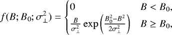 (11)
(11)
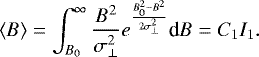
where  is the transverse variance of the magnetic field. Then the mean magnetic field is2
 (12)
(12)
Here  and
and  . We note that I1 is an integral of the form
 (13)
(13)
where  and u = B. Letting t = u2∕a, we have 2udu = adt, so
 (14)
(14)
where  , and we have written the integral as the upper incomplete gamma function
  , with s = 3∕2 and x = t0 (DLMF 2020). Making use of the recurrence relation Γ(s + 1, x) = sΓ(s, x) + xse−x, we have
  . Using the property Γ(1∕2, x) = π1∕2erfc(x1∕2), we get
![Mathematical equation: \begin{equation*} I = \frac{a^{3/2}}{2}\left[\frac{\sqrt{\pi}}{2} \text{erfc}(t_0^{1/2}) + t_0^{1/2} e^{-t_0} \right], \end{equation*}](/articles/aa/full_html/2021/06/aa39816-20/aa39816-20-eq30.png) (15)
(15)
where erfc is the complementary error function. Returning to Eq. (12), we get, after some straightforward algebra,
 (16)
(16)
From Eq. (3) we have, for purely transverse fluctuations,
 (17)
(17)
which may be integrated along the unperturbed, large-scale field line, together with Eq. (16), to obtain the average path length of random-walking field lines. With the assumption of constant δb∕B0 = 1 (or  ) along the field line, the above integral gives ⟨S⟩ = 1.38S0, where S0 is the path length of the central large-scale field line. This estimate is close to the one obtained in Sect. 3.1 from Eq. (10): ⟨S⟩ ~ 1.41S0.
Figure 2 shows four estimates of the path length as a function of the ratio δb∕B0. The shaded regions represent the crude estimates for isotropic and 5:4:1 turbulence derived in Sect. 3.1, with the lower and upper bounds corresponding to the cases of positive and negative δbz, respectively. We note that the upper bounds have a singularity when the denominator of the fractions in Eqs. (7) and (9) vanishes. The figure also compares the two path length estimates for transverse fluctuations; here, ⟨S1⟩ is the simple estimate based on Eq. (10), and ⟨S2⟩ is the rigorous estimate based on Eq. (16). We find that these two estimates are extremely close to each other for δb∕B0 < 1; as δb∕B0 increases, ⟨S1⟩ becomes slightly larger than ⟨S2⟩. Further, we note that, for all four cases, the increase in path length due to FLRW is fractionally small for δb∕B0 ≲ 0.5. For δb∕B0 > 2, the path length can be several times larger than the unperturbed path length for the three non-isotropic cases3. These results suggest that path lengths inferred from SEP observations (see Sect. 5.2) can potentially provide a measure of the prevailing levels of magnetic fluctuations. In Sect. 5.1, we evaluate ⟨S⟩ along a central field line obtained from a global MHD model of the solar wind, taking the spatial variation in B0 and σ⊥ along the field line into account.
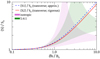 |
Fig. 2 Ratio of path length ⟨S⟩ of random-walking field lines to path length S0 of the unperturbed field line, as a function of δb∕B0. Here ⟨S1⟩ is based on the simple estimate in Sect. 3.1, while ⟨S2⟩ is based on the more rigorous formalism developed in Sect. 3.2; both of these cases are for transverse fluctuations. The pink and green shaded regions represent the cases of isotropic (Eq. (7)) and 5:4:1 (Eq. (9)) fluctuations, respectively. The lower and upper bounds of the shaded regions correspond to the cases of positive and negative δbz, respectively (see Sect. 3.1). |
4 Comparison with Monte Carlo simulations in a model of solar wind magnetic turbulence
4.1 Field line path lengths
Next, we compare the rigorous theoretical result for Gaussian fluctuations from Sect. 3.2 with the path lengths of field lines as traced by a Monte Carlo (MC) simulation based on a model of solar wind magnetic turbulence. This model, previously described by Ruffolo et al. (2013) and Tooprakai et al. (2016), uses a superposition of representations of two turbulence components – a two-dimensional (2D) magnetohydrodynamic (MHD) component and a slab component (Bieber et al. 1994; Seripienlert et al. 2010) – with a radial mean field of strength B0 ∝r−2 in spherical geometry. The fluctuation amplitude is taken to be proportional to B0, with 20% of the fluctuation energy in the slab component and 80% in the 2D MHD component. The only change we made to the model was to consider different values of the rms magnetic fluctuation amplitude δb, setting δb∕B0 = 0.5 (as in previous work) or δb∕B0 = 1, to reflect the strong level of magnetic fluctuation observed near the Sun by PSP (Bale et al. 2019).
Starting at r0 = 0.1 AU, we traced 50 000 magnetic field lines from random heliolongitudes and heliolatitudes within a circle of angular radius 2.5° and measured their incremental path length ΔS over a distance of Δr = 0.25 AU to r = 0.35 AU, which is close to the radius of PSP observations considered in this work.
Since the model uses a constant δb∕B0, even though δb and B0 individually vary as r−2, we expect that the average incremental path length of magnetic field lines over Δr should be

Here, we have made use of Eq. (16) from the rigorous theory for Gaussian fluctuations. In fact, the 2D MHD field that we use does not have a Gaussian distribution of transverse components. The kurtosis of ≈2.7 (Seripienlert et al. 2010) indicates a moderate departure from the Gaussian value of 3, because MHD tends to make the magnetic pressure and magnetic field magnitude more uniform over small scales. Nevertheless, we find that the theory for Gaussian fluctuations from Sect. 3.2 provides a good match for our simulation results.
We also consider a total path length S = ΔS + r0 to account for the field line distance between the Sun and r0. We note that large-scale expansion and magnetic-footpoint motion can potentially increase the path length below r0 = 0.1 AU. Nevertheless, adding a constant r0 to obtain the total path length can be justified to some degree by noting that the Alfvén critical zone, where the solar wind speed roughly equals the Alfvén speed, may be near r ~ 0.1 AU. The solar wind turbulent energy is expected to peak in this region and to be weaker at lower r, where coronal flux tubes may be more rigid (Chhiber et al. 2018, 2019a; Ruffolo et al. 2020). Consequently, in this implementation, and in general, the path length increase due to FLRW is expected to be small in the sub-Alfvénic inner corona, which, according to Moradi & Li (2019), is the case even in the presence of expansion and magnetic-footpoint motion at the solar surface.
Figure 3 shows the simulated distribution of magnetic path length S traced to r = 0.35 AU for the case of δb∕B0 = 1. The average simulated path length ⟨S⟩ is 0.447 AU (vertical dashed line), representing a 28% increase over the distance parallel to the large-scale field. From the theory, we have ⟨B⟩∕B0 = 1.379, which by Eq. (19) implies ⟨ΔS⟩≈ 0.345 AU and ⟨S⟩ ≈ 0.445 AU. This provides a close match to our simulation result. For δb∕B0 = 0.5, we also find good agreement with a simulation result of ⟨S⟩ = 0.382 AU (a 9% increase over the parallel distance) and theory result of ⟨B⟩∕B0 = 1.113 and ⟨S⟩ = 0.378 AU.
For δb∕B0 = 1, Fig. 4 shows the enhancement of the incremental field line path length ⟨ΔS⟩ relative to Δr, the traced distance along the large-scale magnetic field, as a function of Δr. There is an excess in the average field line path length over the theoretical value for short distances. When tracing over Δr = 0.25 AU or longer, the simulation results remain close to the theoretical value.
It is interesting that the theory matches these simulation results well, despite moderate departures from Gaussianity in the dominant magnetic fluctuation component. This agreement gives us greater confidence in applying the theory to address observationsof SEP transport in the actual solar wind.
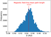 |
Fig. 3 Distribution of path length S of magnetic field lines computationally traced to r = 0.35 AU ina model of solar wind turbulence (a representation of 2D MHD + slab magnetic turbulence in spherical geometry), superposed on a radial mean field of strength B0 ∝ r−2. The rms turbulent amplitude was set equal to the mean field, and the slab energy fraction to 0.2. The vertical dashed line indicates the mean value ⟨S⟩ = 0.447 AU, which is close to our theoretical result of 0.445 AU. |
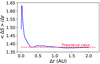 |
Fig. 4 Ratio of average incremental magnetic field line path length ⟨ΔS⟩ to radial distance Δr, as a functionof Δr, for computations described in Fig. 3 and in the text. This ratio is compared with the theoretical ratio of 1.379. |
4.2 Particle guiding-center and full-orbit path lengths
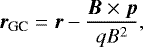
We also performed full-orbit trajectory tracing of 50 000 protons in the same representation of 2D MHD and slab magnetic fluctuations superposed on a radial magnetic field. We measured both the path length s along the full orbit, including the particle gyromotion, and the path length sc of the guiding center. The guiding center location was calculated from the instantaneous particle position r and momentum p from the full orbit particle tracing by
 (20)
(20)
where q is the particle’s electric charge.
We recorded the values of s and sc for particles whenever they crossed the radius of interest in this case r = 0.35 AU. Multiple crossings are included to allow for the backscattering of particles from higher r, as such particles are included in actual SEP observations. Because magnetostatic fluctuations do no work on a particle, the speed (magnitude) v is a constant of the motion. Therefore, the orbit path length beyond r0 can be calculated simply as vt, where t is the time of arrival of the particle at the radius of interest relative to its release from r = r0. The guiding center path length is calculated by summing Δsc from each time step in the simulation. Our simulations start tracing field lines and particles at r0 = 0.1 AU; to account for this and facilitate comparison with SEP observations, we define the total path lengths as s = vt + r0 and sc = ∑ Δsc + r0, and we also added r0 to the magnetic field line path lengths for comparison. The same definition of s was employed by Tooprakai et al. (2016). This effectively assumes that field lines had a negligible fluctuation at r < r0 and that particles traveled along field lines with a zero pitch angle; strong adiabatic focusing (magnetic mirroring) near the Sun tends to make the pitch angle distribution concentrated near zero within r = 0.1 AU (Ruffolo & Khumlumlert 1995), becoming less concentrated thereafter due to pitch angle scattering.
We note that pitch angle scattering is present in the orbit calculation through particle interaction with the slab contribution, which has an adequate spectral bandwidth (2 097 152 Fourier modes) to ensure resonant scattering of the particles at the selected energies. This behavior has been quantified in a number of earlier studies that employ the same methodology (Dalena et al. 2012; Ruffolo et al. 2013; Tooprakai et al. 2016). In addition, as particle orbits are traced through the synthetic turbulent magnetic field, they are not necessarily coupled to any one field line, and the orbits can effectively switch to follow other field lines.
The results for a proton kinetic energy of 25 MeV and δb∕B0 = 1 are shown in Fig. 5. We note that the distribution of the orbit path length s = vt + r0 (black) directly corresponds to the time-intensity profile of an SEP observation. The distribution of the guiding center path length sc corresponds to the time-intensity profile that would be observed if there were no gyromotion, that is, for guiding center transport at pitch angle 0° or 180°. Because of backscattering, both distributions have a “wake” that extends to an indefinitely long path length (or arrival time; Earl 1976). Therefore, we do not use mean values of sc and s to characterize the distributions, and instead consider the peak path lengths and minimum path lengths.
It is interesting to check whether the particle guiding center actually follows a magnetic field line, with the same path length. One might imagine that a particle, with its finite radius of gyration, averages over fluctuations on scales smaller than that radius, and its guiding center might have a shorter path length than the field lines. Indeed, Fig. 5 demonstrates this effect for the case of δb∕B0 = 1, showing that the peak guiding center path length of promptly arriving particles, at ≈ 0.435 AU, is slightly shorter than the average magnetic field line path length ⟨S⟩ = 0.447 AU for the same simulation. In the case of weaker turbulence amplitude, δb∕B0 = 0.5, our simulation results are consistent with no difference between the peak guiding center path length and the average field line path length (both close to 0.38 AU), which in this case are only ≈ 10% longer than the radial distance.
As seen in Fig. 5, the full orbit path length s is distributed over longer values than the guiding center path length sc. In general, this must be the case whenever the pitch angle is nonzero; locally, d sc = |μ|ds where μ is the pitch angle cosine. Here, we find that the nonzero pitch angle and gyromotion of the particles lead to a substantial increase in the particle path length expected for PSP observations, as previously predicted for observations near 1 AU (Lintunen & Vainio 2004; Sáiz et al. 2005).
We note that the minimum full orbit path lengths were presumably associated with near-minimal guiding center path lengths, and the minimum full orbit path lengths are substantially longer. Therefore, even the first arriving particles underwent transport characterized by a nonzero pitch angle. In fact, we can make use of the relation d sc = |μ|ds, assuming that μ >0, to define an effective pitch angle from μeff = sc∕s. For the case shown in Fig. 5, the ratio of either minimum values of sc and s or peak values of these quantities yields essentially the same value of μeff = 0.90–0.91, corresponding to an effective pitch angle θeff ≈ 25°. We have also verified that the distribution of μeff for individual particles, grouped by their orbital path length s, contains no “scatter free” particles with μeff = 1; rather, the distribution is clustered around a mean value that is consistent with the abovementioned ratio and changes very little from the event onset to peak. We emphasize that pitch angle scattering is explicitly included in the particle orbit calculations, and its effects are subsequently characterized in our model in a simplified way. In particular, the effective pitch angle cosine μeff is intended to parameterize the effect of scattering in moving particles away from a zero pitch angle (μ = 1) where they would otherwise likely be clustered due to adiabatic focusing.
In summary, for δb∕B0 = 1 and protons of E = 25 MeV, we find that compared with the total radial distance of 0.35 AU, the average simulated magnetic field line path length is longer by 0.097 AU (due to the FLRW), the peak guiding center path length is shorter than that by about 0.012 AU (due to the gyromotion averaging over fluctuations to some degree), and the peak full orbit path length is longer than that by 0.045 AU (due to the gyromotion itself). Thus in this case, the increase in path length is mainly associated with the FLRW.
For δb∕B0 = 0.5 at the same particle energy, the average simulated magnetic field path length is longer than the radial distance by only 0.032, the peak guiding center path length (≈0.38 AU) is about the same, and the peak full orbit path length (≈0.42 AU) is longer by 0.04 AU. In this case of weaker turbulence, the increase in path length can be attributed, nearly equally, to the field line random walk and the gyromotion.
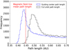 |
Fig. 5 Histograms of simulated path lengths of guiding center motion and full orbital motion for 25 MeV protons arriving promptly at radius r = 0.35 AU from the Sun, for computations described in Fig. 3 and in the text, in comparison with the average path length of magnetic field lines. The guiding center path length of promptly arriving particles (before the arrival of the backscattered population) is usually shorter than the average path length of magnetic field lines because of the finite radius of the gyromotion, which implies that the particle samples the magnetic field over a range of positions and need not exactly follow the random walk of individual field lines. The full orbit path length of the particles is longer because the gyromotion implies that particles follow a longer path than their guiding centers. |
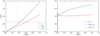 |
Fig. 6 Path length S0 versus heliocentric distance r for a selected large-scale field line from a global heliospheric simulation based on a solar magnetogram for 28 May 2020, compared with two computations of the average path length of random-walking field lines associated with that particular large-scale field line. Here ⟨S1⟩ is based on the simple estimate in Sect. 3.1, while ⟨S2⟩ is based on the more rigorous formalism developed in Sect. 3.2 (see text). Both cases are for transverse fluctuations. In the left panel, the orange vertical line marks the location of PSP at the time of observation of the energetic ion events discussed in Sect. 5.2, and the brown horizontal line marks the particle path length inferred from these observations. See also Fig. 10. |
5 Application of theory to solar energetic particle transport in the solar wind
5.1 Field line path length in global heliospheric simulation
The Usmanov global heliospheric MHD simulation model (Usmanov et al. 2014, 2018) solves compressible three dimensional MHD equations for mean, or large-scale, MHD variables, and incorporates a turbulence transport model that self-consistently interacts with the resolved simulation variables. This code accounts for large-scale features of the interplanetary medium well as observed by Ulysses and Voyager (Usmanov et al. 2012, 2018), as well as turbulence properties observed by PSP (Chhiber et al., in prep.). The code has been used to evaluate energetic particle diffusion coefficients throughout the heliosphere (Chhiber et al. 2017) and to provide several types of contextual predictions for PSP (Chhiber et al. 2019a,b). Because this model provides dynamical solutions for the large-scale magnetic field as well as the rms turbulence amplitude, it can provide all the necessary information to evaluate the magnetic field path lengths using the formulation given in the previous section. Here we use a simulation based on an ADAPT solar magnetogram (Arge et al. 2010), corresponding to 2020 May 28 – the time of the PSP observations examined here. The fluctuations in the turbulence transport model are purely transverse relative to the mean field, and an Alfvén ratio of 0.5 is assumed. For more details on the simulation, including boundary and initial conditions, see Usmanov et al. (2014, 2018).
Figure 6 shows the path length S0 for a selected large-scale field line, compared with two computations of the average path-length of random-walking field lines associated with that particular large-scale field line: The simple estimate ⟨S1⟩ was computed by integrating Eq. (3), using Eq. (10), while the rigorous estimate ⟨S2⟩ was computed using Eq. (17) with ⟨B⟩ specified by Eq. (16). We note that both δb and B0 vary along the field line.
We find that the Parker-spiral-like path length S0 is ~ 1.1 AU at a heliocentric radius of 1 AU, while the path length of random-walking field lines is nearly 2 AU at that distance. Clearly, the FLRW can produce a significant increase in the path length of magnetic field lines, relative to the unperturbed field line. We also note that, for r ≳ 0.4 AU, ⟨S1⟩ becomes noticeably larger than ⟨S2⟩, due to a slight and gradual increase in the ratio δb∕B0 with heliocentric distance (see also Fig. 2). The PSP observations annotated in the left panel of Fig. 6 are discussed in Sect. 5.2, below.
5.2 Application to PSP/IS⊙IS SEP events
The PSP mission is currently on its seventh orbit of the Sun, progressively descending to perihelia deeper in the solar corona with each swing by Venus (Fox et al. 2016). Energetic particle (EP) data from the IS⊙IS suite cover a wide range of energies using two instruments (McComas et al. 2016). EPI-Lo measures energetic ions from 0.02 to ~ 1.5 MeV nuc−1 and energetic electrons of 25–1000 keV. The EPi-Hi instrument measures energetic protons and He nuclei from ~ 1 to ~ 100 MeV nuc−1 (and higher energies for heavier elements) and energetic electrons from ~ 0.5 to ~ 6 MeV. To cover this energy range and to provide wide FOV coverage, EPI-Hi has three telescopes, a double-ended high energy telescope (HET), with apertures HETA and HETB, a double-ended low energy telescope (LET1), with apertures LETA and LETB, and a single-ended low energy telescope (LET2).
During Orbit 5, in a several day period from 2020 May 22 to 2020 June 2, IS⊙IS measured at least six distinct SEP events. These are depicted in Figs. 7 and 8. The orbit and the general features of the energetic particle fluxes measured by IS⊙IS are illustrated in Fig. 7. The EPi-Hi instrument count rates are indicated by bars of varying sizes on the outside of the orbit; the EPi-Lo count rates are given on the inside of the orbit curve. Figure 8 shows data from EPI-Hi and EPI-Lo, andgives more detail on the six easily recognizable energetic particle events during the period from 2020 May 22 (day 143) to 2020 June 2 (day 154). They are numbered in time ordering from 1 to 6. During this target period, PSP was at an approximate Sun-centered radial distance of 0.35 AU. These events are discussed in greater detail in Cohen et al. (2020). We note that for a given particle energy (speed), the intensity versus time in Fig. 8 appears to exhibit a rapid rise to a peak intensity, followed by a more gradual decline, which is qualitatively consistent with the peak and the long “wake” at a later time (longer path length) for particle orbits from the MC simulation (Fig. 8).
To determine an estimated path length for these SEP events, we carried out a standard velocity dispersion analysis, using the data from the LETA and LETB detectors on EPI-Hi. The procedure is to convert the total energy of each measured ion into reciprocal velocity 1∕v and plot it versus the observation time. In this format, the first arriving particles are generally at lower 1∕v (i.e., higher energy), with lower-speed particles arriving later. A straight line fit to the first arriving particles provides a path length (from the slope) and a release time at the source (from thei x-intercept).
The validity of this analysis is based on the assumptions that (i) the first-arriving particles are released from a localized source simultaneously, (ii) they travel the same path length without scattering or energy changes, and (iii) the onset and peak-flux time at the spacecraft is determined accurately (Sáiz et al. 2005). Several studies offer improvements to the basic VDA, including scattering corrections (Laitinen et al. 2015) and the “fractional” VDA, which is applied to times in therising phase of an event that correspond to a varying fraction of the peak flux (Zhao et al. 2019). However, the sharp onset of the events considered here (see Fig. 9) enables an accurate determination of the arrival time. Therefore, for our purposes here, the basic VDA suffices to provide an estimate of the path length.
The two panels of Fig. 9 show such an analysis on 27–28 May (left) for SEP events 3 & 4, and on 29 May (right) for SEP event 5. One readily observes a sharp onset of SEP event 3, starting around five hours prior to 28 May in the left panel. Analysis of the slope of line implies a path length of approximately 0.625 AU from the source to the point of observation at PSP. Transcribing a line with the same slope to the temporal positions of the other events 4 and 5 as shown in Fig. 9 indicates that the same slope, and therefore the same distance from the source to observation,also works well for those cases. This is significantly longer than PSP’s heliocentric distance of about 0.35 AU. We note that a similar result was obtained by Leske et al. (2020) for the SEP event observed by PSP on 4 April 2019, where the inferred path length was 0.35 AU while the spacecraft was at a heliocentric distance of 0.17 AU.
We may employ the analysis described above and the estimation of the field line and particle path lengths given in Sects. 4.2 and 5.1 to offer an explanation of this path length. In fact, three estimates of field line length can be given as described above (see Fig. 6). As before, these are designated as S0, ⟨S1⟩, and ⟨S2⟩. These estimates are depicted in Fig. 10 for the range of distances encompassing PSP’s position at the time of our six targeted events in Fig. 9. We immediately observed that the resolved field line length S0 significantly underestimates the path length derived from the EPI-Hi dispersion analysis in Fig. 9. However, the two estimates derived using the FLRW corrections, which were first based on the average variance ⟨S1⟩ and then based on the more complete stochastic theory ⟨S2⟩ second, revise the estimated path length, moving it substantially closer to the path length obtained from the dispersion analysis.
The remaining deficit relative to the observation is presumably accounted for by particle orbit effects. In Sect. 4.2 we quantified the latter effect for an MC simulation of a test case, finding that the discrepancy between the field line path length and the particle orbit path can be conveniently parameterized by an effective particle pitch angle of 25°. In a similar way, we can estimate an effective pitch angle for the SEP events observed by PSP/IS⊙IS during 2020 May–June. For this estimation, we make two assumptions as follows. (1) Minimum and peak times of particle intensity are very close in time, so we estimate the peak particle orbit path length as 0.625 AU. (2) We neglect the difference in path length between the peak guiding center path length and the average magnetic field path length. With these assumptions, we can estimate that cos (θeff) ≈⟨S2⟩∕(0.625 AU), from which we obtain an effective pitch angle of θeff ≈ 37°. This is not much greater than the value inferred from the MC simulation, and it is not unreasonable that the SEP transport during these events may have been more diffusive than that in the MC simulation4.
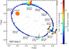 |
Fig. 7 PSP Orbit 5 highlighting SEP events observed by IS⊙IS during 2020 April–July. The count rate is indicated by both the color and the length of the bars, for particles (primarily H+) at lower (about 30– 200 keV; inside track; right color scale) and higher energies (about 1–2 MeV nuc−1; outside track; left color scale). Intervals without data are indicated by the black orbital track. The time scale is indicated by ticks and white rectangles on the outer track as YYYY–DOY (day month), where YYYY is the year, and DOY is the day of the year (UT). |
6 Conclusions
Determining the path length for transit of solar energetic particles from the source to point of observation is a subtle and even elusive problem. Many factors might enter, likely varying from case to case, including free streaming, the curvature and distortion of the large-scale magnetic field, topological trapping, parallel scattering, perpendicular diffusion, subdiffusion, the time dependence of the magnetic field, and FLRW. In this paper, we have chosen to concentrate on two effects which have both been simplified, namely the effect of the average field line length, including FLRW, and the effect of particle gyromotion on the full orbit path length, parameterized by an effective pitch angle.
The FLRW path length sets a natural scale for the problem, even if some of the other effects are also relevant. The orbital path length calculation incorporates a simple treatment of the extension of path length that occurs when particles follow random-walking field lines, but with a nonzero pitch angle, implying a path length systematically longer than the field line length itself.
Our approach consisted of an analytical estimation and validation with numerical tests. First, we developed an exact analytical theory for the average path length using the assumption of classical FLRW, a Gaussian distribution of magnetic fluctuation components, and transverse fluctuations. A simpler estimation based on variances of the magnetic fluctuations is also provided. Figure 2 shows the estimated increase in the path length as a function of the ratio of the fluctuating-to-mean magnetic field. The theory was validated using an MC analysis of an ensemble of field lines in a synthetic turbulence model, with good results. We also carried out an example application using a global heliospheric MHD simulation that includes self-consistent turbulence modeling.
To go beyond the field line path length estimation, we considered particle orbit effects. To this end, a second MC analysis followed test particles (protons) in the same synthetic realization, and the particle path lengths were compared with the field line path lengths, using both guiding center trajectories and exact test particle orbital trajectories. A systematic difference is found – the orbital path lengths being larger – and from this, a correction factor to account for the additional orbital path length is introduced in the form of an effective pitch angle of the particle population as a whole.
Finally the above approach was implemented to examine path lengths inferred from very recent SEP observations by the IS⊙IS instrument suite on PSP (McComas et al. 2016). A dispersion analysis of six SEP events observed by PSP at a heliocentric distance of 0.35 AU in late May and early June 2020 indicates an effective path length of 0.625 AU. To account for this disparity, the FLRW estimation was implemented with the assistance of a global MHD simulation to obtain estimates of local turbulence parameters. This estimate accounts for a little more than half of the added path length inferred from the dispersion analysis. The remainder is accounted for by a plausible effective pitch angle of ~ 37°.
This satisfying result suggests that the easily implemented approach presented here may be useful to provide path length estimates for other SEP events and related observations by PSP and other spacecrafts (e.g., Leske et al. 2020). Conversely, path lengths inferred from observations of SEP events can potentially provide a measure of magnetic turbulence levels, and possibly complement direct measurements of the magnetic field.
In finalizing this paper, it has come to our attention that Laitinen & Dalla (2019) have recently developed a related theoretical approach for computing FLRW influences on the SEP path length. In that case, the method proceeds by solving a stochastic differential equation for the path length, with a final estimated result that depends on the normalized magnetic field variance. An exact analytical result is available only as an approximation. In the future, it will be of interest to compare the results of these two methods, both of which are related to the random walk of magnetic field lines. The related problem of spreading field lines in the direction transverse to the mean field is considered in Chhiber et al. (2021).
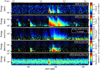 |
Fig. 8 SEP events observed by IS⊙IS from 2020 May 21 (DOY 142) to June 3 (DOY 155), near 0.35 AU. Intensities are indicated by the color scale, as a function of kinetic energy per nucleon and time, for protons (from HETA, top panel; LETA, second panel; and EPI-Lo, third panel), helium (from LETA, fourth panel), and electrons (in counts/sec from HETB, bottom panel). The six events are most clearlyseen in the LETA proton spectrogram (second panel). |
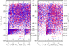 |
Fig. 9 Dispersion analysis of 1∕v versus arrival time for protons during events 3 and 4 (left) and event 5 (right). Each point is a measured proton from either LETA (red) or LETB (blue). The slopes at the onset of each event lead to an estimated path length of about 0.625 AU. |
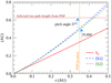 |
Fig. 10 Blow up of Fig. 6, focusing on smaller heliocentric distances. Path length S0 for a large-scale field line from the global solar wind simulation is compared with two computations of path length of random-walking field lines (see caption of Fig. 6). The orange vertical line indicates the approximate radial position of PSP at the time of the events depicted in Fig. 8, and the brown horizontal line depicts the path length derived from the dispersion analysis of these events, shown in Fig. 9. |
Acknowledgements
We thank Junxiang Hu for useful discussions. This research is partially supported by the Parker Solar Probe mission and the IS⊙IS project (contract NNN06AA01C) and a subcontract to University of Delaware from Princeton University (SUB0000165). Additional support is acknowledged from the NASA Living With a Star (LWS) program (NNX17AB79G) and HSR program (80NSSC18K1210 & 80NSSC18K1648) and Thailand Science Research and Innovation (RTA6280002). M.L.G. acknowledges support from the PSP FIELDS MAG team. The IS⊙IS data and visualization tools are available to the community at https://spacephysics.princeton.edu/missions-instruments/isois; data are also available via the NASA Space Physics Data Facility. PSP was designed, built, and is now operated by the Johns Hopkins Applied Physics Laboratory as part of NASA’s LWS program (contract NNN06AA01C). Support from the LWS management and technical team has played a critical role in the success of the PSP mission.
References
- Arge, C. N., Henney, C. J., Koller, J., et al. 2010, AIP Conf. Ser., 1216, 343 [Google Scholar]
- Bale, S. D., Badman, S. T., Bonnell, J. W., et al. 2019, Nature, 576, 237 [Google Scholar]
- Belcher, J. W., & Davis, Jr. L. 1971, J. Geophys. Res., 76, 3534 [Google Scholar]
- Bieber, J. W., & Matthaeus, W. H. 1997, ApJ, 485, 655 [Google Scholar]
- Bieber, J. W., Matthaeus, W. H., Smith, C. W., et al. 1994, ApJ, 420, 294 [Google Scholar]
- Bruno, R., & Carbone, V. 2013, Liv. Rev. Sol. Phys., 10, 2 [Google Scholar]
- Chhiber, R., Subedi, P., Usmanov, A. V., et al. 2017, ApJS, 230, 21 [Google Scholar]
- Chhiber, R., Usmanov, A. V., DeForest, C. E., et al. 2018, ApJ, 856, L39 [Google Scholar]
- Chhiber, R., Usmanov, A. V., Matthaeus, W. H., & Goldstein, M. L. 2019a, ApJS, 241, 11 [Google Scholar]
- Chhiber, R., Usmanov, A. V., Matthaeus, W. H., Parashar, T. N., & Goldstein, M. L. 2019b, ApJS, 242, 12 [Google Scholar]
- Chhiber, R., Ruffolo, D., Matthaeus, W. H., et al. 2021, ApJ, 908, 174 [Google Scholar]
- Chuychai, P., Ruffolo, D., Matthaeus, W. H., & Meechai, J. 2007, ApJ, 659, 1761 [Google Scholar]
- Cohen, C. M. S., Christian, E.R., Cummings, A.C. et al., A&A, 650, A23 (PSP SI) [EDP Sciences] [Google Scholar]
- Dalena, S., Chuychai, P., Mace, R. L., et al. 2012, Comput. Phys. Commun., 183, 1974 [Google Scholar]
- DLMF 2020, NIST Digital Library of Mathematical Functions, http://dlmf.nist.gov/, Release 1.0.27 of 2020-06-15 [Google Scholar]
- Earl, J. A. 1976, ApJ, 206, 301 [Google Scholar]
- Fisk, L. A. 1979, The Interactions of Energetic Particles with the Solar Wind, eds. E. N. Parker, C. F. Kennel, & L. J. Lanzerotti (Amsterdam, North-Holland Publishing Company), 177 [Google Scholar]
- Fox, N. J., Velli, M. C., Bale, S. D., et al. 2016, Space Sci. Rev., 204, 7 [NASA ADS] [CrossRef] [Google Scholar]
- Getmantsev, G. G. 1963, Sov. Astron., 6, 477 [Google Scholar]
- Giacalone, J., Jokipii, J. R., & Mazur, J. E. 2000, ApJ, 532, L75 [Google Scholar]
- Giacalone, J., Jokipii, J. R., & Matthaeus, W. H. 2006, ApJ, 641, L61 [Google Scholar]
- Hartlep, T., Matthaeus, W. H., Padhye, N. S., & Smith, C. W. 2000, J. Geophys. Res., 105, 5135 [Google Scholar]
- Isichenko, M. B. 1991, Plasma Phys. Control. Fusion, 33, 809 [Google Scholar]
- Jokipii, J. R. 1966, ApJ, 146, 480 [Google Scholar]
- Jokipii, J. R., & Parker, E. N. 1969, ApJ, 155, 777 [Google Scholar]
- Kadomtsev, B. B., & Pogutse, O. P. 1979, in Plasma Physics and Controlled Nuclear Fusion Research (Berlin: Springer), 1, 649 [Google Scholar]
- Kóta, J., & Jokipii, J. R. 2000, ApJ, 531, 1067 [Google Scholar]
- Laitinen, T., & Dalla, S. 2017, ApJ, 834, 127 [Google Scholar]
- Laitinen, T., & Dalla, S. 2019, ApJ, 887, 222 [Google Scholar]
- Laitinen, T., Dalla, S., & Marsh, M. S. 2013, ApJ, 773, L29 [Google Scholar]
- Laitinen, T., Huttunen-Heikinmaa, K., Valtonen, E., & Dalla, S. 2015, ApJ, 806, 114 [Google Scholar]
- Leske, R. A., Christian, E. R., Cohen, C. M. S., et al. 2020, ApJS, 246, 35 [Google Scholar]
- Lingenfelter, R. E., Ramaty, R., & Fisk, L. A. 1971, Astrophys. Lett., 8, 93 [Google Scholar]
- Lintunen, J., & Vainio, R. 2004, A&A, 420, 343 [NASA ADS] [CrossRef] [EDP Sciences] [Google Scholar]
- Matthaeus, W. H., Qin, G., Bieber, J. W., & Zank, G. P. 2003, ApJ, 590, L53 [Google Scholar]
- McComas, D. J., Alexander, N., Angold, N., et al. 2016, Space Sci. Rev., 204, 187 [Google Scholar]
- Minnie, J., Matthaeus, W. H., Bieber, J. W., Ruffolo, D., & Burger, R. A. 2009, J. Geophys. Rese. Space Phys., 114, A01102 [Google Scholar]
- Montgomery, D. 1982, Phys. Scr., T2A, 83 [Google Scholar]
- Moradi, A., & Li, G. 2019, ApJ, 887, 102 [Google Scholar]
- Oughton, S., Matthaeus, W. H., & Dmitruk, P. 2017, ApJ, 839, 2 [Google Scholar]
- Qin, G., Matthaeus, W. H., & Bieber, J. W. 2002a, ApJ, 578, L117 [Google Scholar]
- Qin, G., Matthaeus, W. H., & Bieber, J. W. 2002b, Geophys. Res. Lett., 29, 1048 [Google Scholar]
- Ragot, B. R. 2006, ApJ, 653, 1493 [Google Scholar]
- Rappazzo, A. F., Velli, M., Einaudi, G., & Dahlburg, R. B. 2008, ApJ, 677, 1348 [Google Scholar]
- Ruffolo, D., & Khumlumlert, T. 1995, Geophys. Res. Lett., 22, 2073 [Google Scholar]
- Ruffolo, D., Matthaeus, W. H., & Chuychai, P. 2003, ApJ, 597, L169 [Google Scholar]
- Ruffolo, D., Chuychai, P., Wongpan, P., et al. 2008, ApJ, 686, 1231 [Google Scholar]
- Ruffolo, D., Pianpanit, T., Matthaeus, W. H., & Chuychai, P. 2012, ApJ, 747, L34 [Google Scholar]
- Ruffolo, D., Seripienlert, A., Tooprakai, P., Chuychai, P., & Matthaeus, W. H. 2013, ApJ, 779, 74 [Google Scholar]
- Ruffolo, D., Matthaeus, W. H., Chhiber, R., et al. 2020, ApJ, 902, 94 [Google Scholar]
- Sáiz, A., Evenson, P., Ruffolo, D., & Bieber, J. W. 2005, ApJ, 626, 1131 [Google Scholar]
- Seripienlert, A., Ruffolo, D., Matthaeus, W. H., & Chuychai, P. 2010, ApJ, 711, 980 [Google Scholar]
- Shalchi, A. 2009, Nonlinear Cosmic Ray Diffusion Theories (Berlin: Springer), 362 [CrossRef] [Google Scholar]
- Shalchi, A. 2010, ApJ, 720, L127 [Google Scholar]
- Sonsrettee, W., Subedi, P., Ruffolo, D., et al. 2015, ApJ, 798, 59 [Google Scholar]
- Sonsrettee, W., Subedi, P., Ruffolo, D., et al. 2016, ApJS, 225, 20 [Google Scholar]
- Subedi, P., Sonsrettee, W., Blasi, P., et al. 2017, ApJ, 837, 140 [Google Scholar]
- Taylor, J. B., & McNamara, B. 1971, Phys. Fluids, 14, 1492 [Google Scholar]
- Tooprakai, P., Chuychai, P., Minnie, J., et al. 2007, Geophys. Res. Lett., 34, L17105 [Google Scholar]
- Tooprakai, P., Seripienlert, A., Ruffolo, D., Chuychai, P., & Matthaeus, W. H. 2016, ApJ, 831, 195 [Google Scholar]
- Urch, I. H. 1977, Ap&SS, 46, 389 [Google Scholar]
- Usmanov, A. V., Goldstein, M. L., & Matthaeus, W. H. 2012, ApJ, 754, 40 [Google Scholar]
- Usmanov, A. V., Goldstein, M. L., & Matthaeus, W. H. 2014, ApJ, 788, 43 [Google Scholar]
- Usmanov, A. V., Matthaeus, W. H., Goldstein, M. L., & Chhiber, R. 2018, ApJ, 865, 25 [Google Scholar]
- Webb, G. M., Zank, G. P., Kaghashvili, E. K., & le Roux, J. A. 2006, ApJ, 651, 211 [Google Scholar]
- Zhao, L., Li, G., Zhang, M., et al. 2019, ApJ, 878, 107 [Google Scholar]
A similar approach was used by Ragot (2006) to estimate the average length of meandering field lines; they used a Gaussian distribution of field-line displacements, instead of the distribution of fluctuations used here.
We note that  , where as ⟨B⟩≡⟨|B|⟩, where
 . For purely transverse fluctuations, bz = 0.
It is important to recall that the isotropic case is not generally of relevance to the solar wind, but it could have implications for astrophysical systems (Subedi et al. 2017, and references therein). We also note that the turbulence is not generally isotropic unless δb∕B0 ≫ 1 and, therefore, the large path lengths seen for the isotropic case in Fig. 2 may not be physically relevant in the context of the crude model in Sect. 3.1.
We note that the MC simulation used a constant δb∕B0, while this ratio spatially varies in the global solar wind simulation.
All Figures
|
Fig. 1 Schematic showing central and random-walking field lines emerging from the Sun, and the local coordinate system used. We note that the magnetic field is statistically axisymmetric about the mean-field direction
|
| In the text | |
|
Fig. 2 Ratio of path length ⟨S⟩ of random-walking field lines to path length S0 of the unperturbed field line, as a function of δb∕B0. Here ⟨S1⟩ is based on the simple estimate in Sect. 3.1, while ⟨S2⟩ is based on the more rigorous formalism developed in Sect. 3.2; both of these cases are for transverse fluctuations. The pink and green shaded regions represent the cases of isotropic (Eq. (7)) and 5:4:1 (Eq. (9)) fluctuations, respectively. The lower and upper bounds of the shaded regions correspond to the cases of positive and negative δbz, respectively (see Sect. 3.1). |
| In the text | |
|
Fig. 3 Distribution of path length S of magnetic field lines computationally traced to r = 0.35 AU ina model of solar wind turbulence (a representation of 2D MHD + slab magnetic turbulence in spherical geometry), superposed on a radial mean field of strength B0 ∝ r−2. The rms turbulent amplitude was set equal to the mean field, and the slab energy fraction to 0.2. The vertical dashed line indicates the mean value ⟨S⟩ = 0.447 AU, which is close to our theoretical result of 0.445 AU. |
| In the text | |
|
Fig. 4 Ratio of average incremental magnetic field line path length ⟨ΔS⟩ to radial distance Δr, as a functionof Δr, for computations described in Fig. 3 and in the text. This ratio is compared with the theoretical ratio of 1.379. |
| In the text | |
|
Fig. 5 Histograms of simulated path lengths of guiding center motion and full orbital motion for 25 MeV protons arriving promptly at radius r = 0.35 AU from the Sun, for computations described in Fig. 3 and in the text, in comparison with the average path length of magnetic field lines. The guiding center path length of promptly arriving particles (before the arrival of the backscattered population) is usually shorter than the average path length of magnetic field lines because of the finite radius of the gyromotion, which implies that the particle samples the magnetic field over a range of positions and need not exactly follow the random walk of individual field lines. The full orbit path length of the particles is longer because the gyromotion implies that particles follow a longer path than their guiding centers. |
| In the text | |
|
Fig. 6 Path length S0 versus heliocentric distance r for a selected large-scale field line from a global heliospheric simulation based on a solar magnetogram for 28 May 2020, compared with two computations of the average path length of random-walking field lines associated with that particular large-scale field line. Here ⟨S1⟩ is based on the simple estimate in Sect. 3.1, while ⟨S2⟩ is based on the more rigorous formalism developed in Sect. 3.2 (see text). Both cases are for transverse fluctuations. In the left panel, the orange vertical line marks the location of PSP at the time of observation of the energetic ion events discussed in Sect. 5.2, and the brown horizontal line marks the particle path length inferred from these observations. See also Fig. 10. |
| In the text | |
|
Fig. 7 PSP Orbit 5 highlighting SEP events observed by IS⊙IS during 2020 April–July. The count rate is indicated by both the color and the length of the bars, for particles (primarily H+) at lower (about 30– 200 keV; inside track; right color scale) and higher energies (about 1–2 MeV nuc−1; outside track; left color scale). Intervals without data are indicated by the black orbital track. The time scale is indicated by ticks and white rectangles on the outer track as YYYY–DOY (day month), where YYYY is the year, and DOY is the day of the year (UT). |
| In the text | |
|
Fig. 8 SEP events observed by IS⊙IS from 2020 May 21 (DOY 142) to June 3 (DOY 155), near 0.35 AU. Intensities are indicated by the color scale, as a function of kinetic energy per nucleon and time, for protons (from HETA, top panel; LETA, second panel; and EPI-Lo, third panel), helium (from LETA, fourth panel), and electrons (in counts/sec from HETB, bottom panel). The six events are most clearlyseen in the LETA proton spectrogram (second panel). |
| In the text | |
|
Fig. 9 Dispersion analysis of 1∕v versus arrival time for protons during events 3 and 4 (left) and event 5 (right). Each point is a measured proton from either LETA (red) or LETB (blue). The slopes at the onset of each event lead to an estimated path length of about 0.625 AU. |
| In the text | |
|
Fig. 10 Blow up of Fig. 6, focusing on smaller heliocentric distances. Path length S0 for a large-scale field line from the global solar wind simulation is compared with two computations of path length of random-walking field lines (see caption of Fig. 6). The orange vertical line indicates the approximate radial position of PSP at the time of the events depicted in Fig. 8, and the brown horizontal line depicts the path length derived from the dispersion analysis of these events, shown in Fig. 9. |
| In the text | |
Current usage metrics show cumulative count of Article Views (full-text article views including HTML views, PDF and ePub downloads, according to the available data) and Abstracts Views on Vision4Press platform.
Data correspond to usage on the plateform after 2015. The current usage metrics is available 48-96 hours after online publication and is updated daily on week days.
Initial download of the metrics may take a while.