| Issue |
A&A
Volume 650, June 2021
Parker Solar Probe: Ushering a new frontier in space exploration
|
|
|---|---|---|
| Article Number | A5 | |
| Number of page(s) | 10 | |
| Section | The Sun and the Heliosphere | |
| DOI | https://doi.org/10.1051/0004-6361/202039806 | |
| Published online | 02 June 2021 | |
Direct evidence for magnetic reconnection at the boundaries of magnetic switchbacks with Parker Solar Probe
1
LPC2E, CNRS/University of Orléans/CNES,
3A avenue de la Recherche Scientifique,
Orléans, France
e-mail: This email address is being protected from spambots. You need JavaScript enabled to view it.
2
Space Sciences Laboratory, University of California,
Berkeley,
CA 94720-7450, USA
3
Institut de Recherche en Astrophysique et Planétologie, CNRS, UPS, CNES,
Toulouse, France
4
Laboratoire d’Astrophysique de Bordeaux, Univ. Bordeaux, CNRS, B18N, allée Geoffroy Saint-Hilaire,
33615
Pessac, France
5
National Institute for Astrophysics-Institute for Space Astrophysics and Planetology,
Via del Fosso del Cavaliere 100,
00133
Roma, Italy
6
Department of Earth, Planetary, and Space Sciences, UCLA,
Los Angeles,
CA 90095, USA
7
Laboratory for Atmospheric and Space Physics, University of Colorado,
Boulder,
CO 80303, USA
8
Astrophysical and Planetary Sciences Department, University of Colorado,
Boulder,
CO 80303, USA
9
Physics Department, University of California,
Berkeley,
CA 94720-7300, USA
10
The Blackett Laboratory, Imperial College London,
London,
SW7 2AZ, UK
11
School of Physics and Astronomy, Queen Mary University of London,
London
E1 4NS, UK
12
Smithsonian Astrophysical Observatory,
Cambridge,
MA 02138, USA
13
School of Physics and Astronomy, University of Minnesota,
Minneapolis,
MN 55455, USA
14
Climate and Space Sciences and Engineering, University of Michigan,
Ann Arbor,
MI 48109, USA
15
BWX Technologies, Inc.,
Washington,
DC 20002, USA
16
Solar System Exploration Division, NASA/Goddard Space Flight Center,
Greenbelt,
MD 20771, USA
Received:
30
October
2020
Accepted:
15
January
2021
Abstract
Context. The first encounters of Parker Solar Probe (PSP) with the Sun revealed the presence of ubiquitous localised magnetic deflections in the inner heliosphere; these structures, often called switchbacks, are particularly striking in solar wind streams originating from coronal holes.
Aims. We report the direct piece of evidence for magnetic reconnection occurring at the boundaries of three switchbacks crossed by PSP at a distance of 45 to 48 solar radii to the Sun during its first encounter.
Methods. We analyse the magnetic field and plasma parameters from the FIELDS and Solar Wind Electrons Alphas and Protons instruments.
Results. The three structures analysed all show typical signatures of magnetic reconnection. The ion velocity and magnetic field are first correlated and then anti-correlated at the inbound and outbound edges of the bifurcated current sheets with a central ion flow jet. Most of the reconnection events have a strong guide field and moderate magnetic shear, but one current sheet shows indications of quasi anti-parallel reconnection in conjunction with a magnetic field magnitude decrease by 90%.
Conclusions. Given the wealth of intense current sheets observed by PSP, reconnection at switchback boundaries appears to be rare. However, as the switchback boundaries accomodate currents, one can conjecture that the geometry of these boundaries offers favourable conditions for magnetic reconnection to occur. Such a mechanism would thus contribute in reconfiguring the magnetic field of the switchbacks, affecting the dynamics of the solar wind and eventually contributing to the blending of the structures with the regular wind as they propagate away from the Sun.
Key words: Sun: heliosphere / solar wind / magnetic fields / magnetic reconnection
© C. Froment et al. 2021
 Open Access article, published by EDP Sciences, under the terms of the Creative Commons Attribution License (https://creativecommons.org/licenses/by/4.0), which permits unrestricted use, distribution, and reproduction in any medium, provided the original work is properly cited.
1 Introduction
The solar atmosphere constantly releases a stream of particles, known as the solar wind. How these particles are accelerated to the interplanetary medium is still an open question. Parker Solar Probe (PSP, Fox et al. 2016) is the first spacecraft to go close enough to the Sun to sample the in situ characteristics of the pristine solar wind in order to tackle this question. During the first encounter of PSP with the Sun, in November 2018, the spacecraft was embedded in a slow-wind stream originating from a small coronal hole (Riley et al. 2019; Badman et al. 2020; Kim et al. 2020; Szabo et al. 2020) and made an approach at 35.7 solar radii. These observations revealed the ubiquitous presence of deflections in the magnetic field of the solar wind (Bale et al. 2019), which are particularly pronounced in the variation of its radial component. Although most deflections (from the prevalent sunward polarity) are of a few tens of degrees, some correspond to full reversals (Dudok de Wit et al. 2020; Mozer et al. 2020). Their duration spans from a few seconds to a few hours (Dudok de Wit et al. 2020). For these structures the electron pitch-angle distributions show that the strahl, the high energy electron population emanating from the Sun, follows the orientation of the magnetic field (Kasper et al. 2019). This suggest that these ‘switchbacks’ are localised twists in the magnetic field and not simple polarity reversals or closed loops. Cross helicity measurements, in addition, show that magneto-hydrodynamic waves follow the magnetic field inside the switchbacks (McManus et al. 2020). This magnetic field twist is coupled with a proton velocity enhancement that is most of the time, but not always, of the order of the local Alfvén velocity. As shown by Larosa et al. (2021), velocity enhancements inside switchbacks can be only of a few percent of the velocity outside of the structures. The statistics of these enhancements show a continuum of fractions of the local Alfvén velocity.
Structures similar to switchbacks were observed before in the solar wind (e.g Balogh et al. 1999; Horbury et al. 2018). However, the new observations from PSP revealed persistent features, populating a significant fraction of the measurements. Such short events had also never been observed before. The scattered observation of switchbacks further away from the Sun could be due to their deterioration as they travel, even though these structures seem to be able to live long enough in the slow solar wind to be generated close to the Sun and observed at a few tens of solar radii (Tenerani et al. 2020a). The ubiquity of switchbacks in PSP observations (also during subsequent perihelia) could also be due to the co-rotation of the probe with the Sun during the encounters, allowing the probe to meet a larger number of them, even if they were emitted by a rather localised source on the Sun (Horbury et al. 2020). We also note that there is presently no consensus between the few statistical studies that have quantified the degree of occurrence of switchbacks with the radial distance from the Sun (Tenerani et al. 2020b; Velli et al. 2020).
Observational studies invoke the formation of these structures either by processes occurring deep in the solar atmosphere (Dudok de Wit et al. 2020; Krasnoselskikh et al. 2020; Macneil et al. 2020; Woodham et al. 2021) or directly in the solar wind (Ruffolo et al. 2020). These two types of origins have also been explored on the numerical and theoretical side: on the one hand, via interchange reconnection in the corona (Fisk & Kasper 2020; Drake et al. 2021) or jets in the solar atmosphere (Roberts et al. 2018; Sterling & Moore 2020; He et al. 2020); on the other hand, via waves growth generated by the expansion of the structure away from the Sun (Squire et al. 2020) or shear-driven turbulence in the solar wind (Ruffolo et al. 2020). As of today, the mechanisms leading to the formation of switchbacks is still unclear and it is unknown whether different populations of switchbacks might be generated by distinct mechanisms. Their omnipresence, however, shows that they could play an important role in the dynamics and heating of the solar wind.
Several interesting properties of the switchbacks arise from the study of their boundaries. The rotation of the magnetic field at the boundary of switchbacks make them current sheets by definition. Via a superposed epoch analysis, Farrell et al. (2020) highlight that events with a rapid deflection in the magnetic field show a clear decrease in the magnetic field magnitude at their boundaries (7–8%). The authors conjecture that these dropouts are caused by a diamagnetic current created at the boundaries by a pressure gradient in the region where the magnetic field is rotating. This kind of magnetic field dropout coupled with a proton density increase at switchback boundaries were clearly present in several studies (e.g Bale et al. 2019; Krasnoselskikh et al. 2020; Agapitov et al. 2020). Krasnoselskikh et al. (2020) have also reported strong currents at switchback boundaries, which is confirmed by the statistical analysis conducted by Larosa et al. (2021).
Current sheets are privileged regions for magnetic reconnection to occur. In the case of magnetic reconnection, the magnetic field topology is reconfigured to a simpler configuration, converting magnetic energy into thermal and kinetic energies (e.g Cassak 2016; Zweibel & Yamada 2009, 2016). Particles are ejected away from the reconnection site at a velocity close to the Alfvén velocity, and the plasma is locally heated. Reconnection in the solar wind is typically detected through the observation of an ion flow jet within a bifurcated current sheet (Gosling et al. 2005). The probability of crossing the reconnection site, the so-called diffusion region, is low due to its small spatial scale (of the order of the ion inertial length di). A correlation between the evolution of the magnetic field and the particle density, later followed by an anti-correlation, or the other way around, is typically observed when reconnection exhausts are crossed. Such behaviour is consistent with Alfvén waves propagating along the magnetic field, away from the reconnection site on either side of the exhaust, as demonstrated by Gosling et al. (2005). In PSP observations, reconnection exhausts have been reported at the heliospheric current sheets (HCS), in interplanetary coronal mass ejections (ICME), and in some isolated current sheets, but not so far at the most frequent current sheets observed which are those that bound switchbacks (e.g. Phan et al. 2020; Lavraud et al. 2020; Fargette et al. 2021).
In this paper, we analyse the boundaries of three switchbacks that were crossed during the first solar encounter of PSP. At least five out of six current sheets show direct evidence of magnetic reconnection. They were observed on November 1 and November 2, 2018, that is to say five and four days before perihelion. At that time, PSP was located between 48 and 45 solar radii from the Sun. The observations are presented in Sect. 2. After the detailed analysis of the three events in Sect. 3, we summarise their properties and discuss the implications of our observations on the switchbacks dynamics and propagation in the solar wind in Sect. 4.
2 PSP observations
2.1 Data
We used magnetic field measurements made by the FIELDS suite of instruments (Bale et al. 2016). The vector magnetic field was measured from DC to several tens of hertz by the fluxgate magnetometer (MAG) while magnetic fluctuations above 10 Hz were measured by the Search-Coil Magnetometer (SCM, Jannet et al. 2021). Our analysis of wave activity (Sect. 3.2) and its properties is based on waveforms (73.24 samples per second, 3 components), auto- and cross-spectra (cadence of 28 s, full spectralmatrix), and band-pass filter (BPF) time series (cadence of 0.87 s, one component only: u in the SCM sensor frame) of the search-coil. BPF time series represent the amplitude of the wavefield in specific spectral bands. All these data products are provided by the Digital Fields Board (DFB, Malaspina et al. 2016). The sampling rate of the waveforms corresponds to the survey cadence during the early part of the solar encounter phase. During the close encounter phase, this cadence increases fourfold. However, none of the switchback boundaries observed during the close encounter show as clear evidence for reconnection as the ones that we present below.
The proton velocity, density, and temperature are provided by the Solar Wind Electrons Alphas and Protons (SWEAP) suite (Kasper et al. 2016). SPC Faraday cups (Case et al. 2020) provide moments of the reduced distribution function of ions: density, velocity, and radial component of the thermal velocity. From the latter, we estimated the radial proton temperature:  [eV], where kB is the Boltzmann constant, Mi is the mass of protons, and δv2 is the proton radial thermal velocity. These data come with different quality flags; we only used good quality data. Their cadence is 0.22 s. Finally, we considered the electron pitch angle distribution at 314 eV from the Solar Probe ANalyzer-Electron (SPAN-E, Whittlesey et al. 2020), whose cadence is 28 s.
2.2 Coordinate systems
Throughout our analysis, we used different coordinate systems. RTN coordinates were used for the analysis of switchbacks and their boundaries: R is radial and points away from the Sun, the tangential T component is the cross-product of the solar rotation vector with R; and the normal N component completes the right-handed set and points in the same direction as the solar rotation vector.
For the analysis of the current sheets, we expressed the magnetic field and proton velocity measurements in the local current sheet coordinate system, LMN: L being the main direction of the current sheet, M the out-of-plane direction, and N the normal. We followed the same hybrid minimum variance method as described in Phan et al. (2020, Sect. 2.3), using the two points enclosing the abrupt change in BR as references for the calculations.
3 Evidence for magnetic reconnection at the boundaries of magnetic switchbacks
Here, we present the analysis of three magnetic switchbacks showing evidence for magnetic reconnection at their boundaries. The selection of the events was made through visual inspection of a large list of switchbacks. We do not aim here to present an exhaustive detection of such events. They seem rare, and the cases we report here are the most striking ones.
3.1 Reconnection exhausts with strong guide field
The two switchbacks that are presented in this section show strong similarities and are thus grouped together here. As we detail, strong pieces of evidence for magnetic reconnection are detected at both edges of these switchbacks.
3.1.1 Event 1 on November 2, 2018 at 13:05:09 UT
Figure 1 shows the main features observed during the crossing of the switchback constituting event 1, observed on November 2, 2018. The leading edge crossing started at 13:05:09 UT and the trailing edge one started at 13:15:11 UT. These crossings, which last 5.6 ± 0.5 s and 7.9 ± 0.5 s, respectively, are highlighted with a light red shaded area in Fig. 1. These windows correspond to the abrupt changes in BR. For this switchback, the total crossing time was about 10 min.
We note that BR went from about − 42 nT to a maximum of 8 nT inside the structure. We note that BR dropped again to a negative value inside the structure, that is − 52 nT, which is approximately the value reached after the crossing of the structure. The average radial proton velocity during this time window was 320 km s−1, with a clear enhancement inside the switchback with vR varying from about 312 km s−1 before the switchback, up to 352 km s−1 inside. This velocity enhancement is smaller than the local Alfvén velocity, even though the minimal changes in |B | and strong correlation between BR and vR evoke a quasi-Alfvénic perturbation.
The electron pitch angle distribution (PAD) at 314 eV shows higher fluxes at a pitch angle of 180° (anti-field aligned) before, during and after the crossing of the structure. Such a constant PAD behaviour is a typical feature of a switchback. It reveals the local kink in the magnetic field structure (see Sect. 1).
Jets, mainly in the R and N components of the proton velocity, are clearly visible at both edges of the structure. In the two sets of plots at the bottom of Fig. 1, we show close-ups of the two boundaries treated as current sheets. The magnetic field and proton density are now expressed in the respective local current sheet coordinate system: LMN. In this frame, we now compare the evolution of BL and vL, that is the magnetic field and proton velocity along the current sheet, at the two boundaries of the switchback. We note that for both current sheets, the guide field BM was strong compared to the reconnecting field BL: 2.3 and 1.3 times higher, respectively.
At the leading edge, the proton jet now seen in the main direction of the current sheet has a ΔvL = −52 km s−1, which in an absolute value represents approximately 50% of the local Alfvén velocity. For this boundary, we do not notice any significant density or radial temperature increase spanning multiple data points.
At the trailing edge, the proton jet has a ΔvL = +107 km s−1, that is 113% of the local Alfvén velocity. For this boundary there is a significant increase in the proton density of 20%. As for the other boundary, there are no significant variations in the radial temperature.
We now compare the relative variations of BL and vL in order to check whether there are correlated variations. This analysis is displayed in Fig. 2 for both the leading and trailing current sheets. Here, BL was decimated to the cadence of vL. Next, we computed the Pearson correlation coefficient between BL and vL for time windows that delimit the boundaries. For each current sheet, these time windows were chosen in such a way as to maximise the correlation coefficient.
For the leading edge, we find a positive correlation of 0.65 between BL and vL, followed by an anti-correlation of −0.79. For the trailing edge, we observe the same succession: a positive correlation of 0.97 followed by an anti-correlation of −0.87.
A change of sign in the correlation between BL and vL is expected for reconnection exhausts (see Sect. 1). Together with the associated proton jet they provide direct evidence for reconnection at the boundaries of the switchback. We note that the trailing edge current sheet had already been reported by Phan et al. (2020) as a regular solar wind event (i.e. not linked to a particular structure as an HCS crossing or ICME).
3.1.2 Event 2 on November 1, 2018 at 23:23:04 UT
Event 2 was registered on November 1, 2018. The crossing of the leading edge occurred at 23:23:04 UT and lasted 3.8 ± 0.5 s. PSP crossed the trailing edge at 23:25:01 UT for 27.7 ± 0.5 s. This second boundary is large and has several sub-structures. The crossing of the switchback itself lasted for 1 min and 50 s in total, which is considerably faster than for event 1. Event 2 is presented in Fig. 3.
We note that BR went from approximately −30 nT before the switchback, to +37 nT inside the structure. The magnitude of proton velocity also increased inside the switchback by about 10 km s−1 compared the velocity before the crossing. The PAD properties remain constant throughout the structure as for event 1, which is expected for magnetic switchbacks. We note that this structure is embedded in a larger switchback, which we present in Fig. 4. The crossing of this larger switchback started at 23:16:59 UT and ended at 23:25:29 UT. Analysing the properties of this complex structure is beyond the scope of the present paper, but we note that this structure shows overall an increase in |B | and decrease in the proton density with anti-correlation between these two variables. This is consistent with the slow magnetosonic perturbations reported in Larosa et al. (2021).
Going back now to the sub-structure constituting event 2, from the measurements in the RTN frame only, it is already clear that both boundaries show proton jets, with an increase and a decrease in velocity, respectively.In the local current sheet coordinate system, it appears that these current sheets also had a strong guide field: 2.3 and 2.6 times the reconnecting field, respectively. The jet at the leading edge has a ΔvL = +22 km s−1, that is 26% of the local Alfvén velocity. For the trailing edge, ΔvL = −52 km s−1, that is 60% of the local Alfvén velocity. No clear density nor radial temperature variations were observed, except for the 41% proton density increase at the trailing edge. We present the correlated variations of BL and vL in Fig. 5. At the leading edge, the positive correlation (0.95) is followed by an anti-correlation (–0.80). The same occurs at the trailing edge, with a correlation (0.96), followed by an anti-correlation (−0.76).
We conclude that both boundaries of this switchback also undergo magnetic reconnection. We note that these events were also reported by Phan et al. (2020) as regular solar wind events.
We similarly analysed the leading edge of the larger structure presented in Fig. 4. No evidence for reconnection was found in that current sheet.
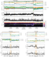 |
Fig. 1 Event 1 on November 2, 2018, starting at 13:05:09 UT. The shaded areas delimit the boundaries of the switchback, noted as leading and trailing edges. First panel: DC magnetic field measurements from FIELDS/MAG in the RTN frame. Second panel: proton velocity from SWEAP/SPC, also in the RTN frame. The average value of the radial velocity (⟨vR ⟩ = 320 km s−1) was removed for easier visualisation. Third panel: proton density from SWEAP/SPC. Fourth panel: radial proton temperaturefrom SWEAP/SPC. Fifth panel: pitch angle distribution of 314 eV electrons from SWEAP/SPAN-E. The combined flux (two sensors) was normalised by the averaged flux. The white curve represents the magnitude of the magnetic field in arbitrary units. Bottom panels: two sets of plots at the bottom are excerpts of the leading and trailing edges of theswitchback; they represent the same variables (except for the pitch-angle distribution) in the same order. For these two sets of plots, the magnetic field and proton velocity are represented in the local current sheet coordinates LMN. The average value of the velocity for each component was removed for easier visualisation. |
 |
Fig. 2 Correlation and anti-correlation of BL and vL at the boundaries of event 1. The leading edge is represented in the left panel and trailing edge in the right panel. Evolution of BL and vL, component along the main direction of the current sheets. The Pearson correlation coefficients shown were computed in the coloured time windows, chosen to maximise the correlation values. The light brown line is the magnitude of the magnetic field. |
3.2 Event 3 on November 1, 2018 at 18:18 UT
First, we present the context for event 3 in Fig. 6. This magnetic structure is close to a full reversal of the magnetic field, with a rotation of B of approximately 165°. We note that BR goes from about –30 nT before the switchback to +40 nT inside and then back, close to its original value. For this structure there is also a full reversal of BT and a large deflection in BN. The inner part of the switchback is highly structured, with several smaller deflections in the field. However, we do not consider these sub-structures and focus on the structure as a whole.
PSP crossed the leading and trailing edges of the switchback at approximately 18:21:28 UT and 18:34:39 UT, respectively. These crossings lasted for about 6.0 ± 0.5 s and 16.2 ± 0.5 s, respectively. The total crossing time of the structure is about 13 min. For both boundaries, there is a strong decrease in the magnitude of the magnetic field by about 90%, down to 3 nT.
The average radial proton velocity during this time window is 342 km s−1, with a clear enhancement inside the switchback with vR varying from about −40 to 40 km s−1, which is an increase that is close to the local Alfvén velocity. The proton density inside the structure decreases from about 200 to 150 cm−3 but shows a local increase of about 15% at the trailing edge. This behaviour is consistent with the observation of typical switchbacks with magnetic decreases at their boundaries (Farrell et al. 2020). However, here, there is no clear increase in the proton temperature. We note that alongside the strong decrease in |B |, there is no dramatic increase in the proton density and almost none in the proton temperature. Consequently, βp is high at the switchback boundaries, reaching 68 and 113 at the points of reversal, respectively.
We notea suppression of the strahl at both boundaries. It is particularly striking at the trailing edge where around the minimum in |B |, the flux is weak and not field-aligned. Since the magnetic field direction is changing quickly with respect to the sampling period of SPAN-E, one has to be careful with the interpretation. Meanwhile, we also see a decrease in the electron flux in the two neighbouring bins of the magnetic dip. Additionally, we meticulously checked that the rotation of the magnetic field in these bins is properly captured in the data used to compute the PADs. From these analyses, we conclude that the strahl dropouts are real and are not due to data processing.
We now focus on the boundaries of the switchbacks. As described above, they share similarities: large magnetic field dips; changes in the strahl; a very high value of βp; and a small increase in the proton density. However, the configuration of the magnetic field at the trailing edge is verydifferent as it shows a full reversal of the three components with a large magnetic shear of 168°. Combined with the strong decrease in magnitude, this could indicate that PSP was very close to an X-point.
For the leading edge, the current sheet crossing lasts about 0.7 s, which is not enough to resolve a possible reconnection process (only three data points in the SWEAP measurements). However, we notice a velocity enhancement, although on only one point, which may be the signature of a reconnection jet. For this point at the middle of the current sheet, ΔvL = 35 km s−1, which is about 75% of the local Alfvén velocity. Although not resolved, the presence of this jet is consistent with a change in sign for the correlation between BL and vL, which is expected forreconnection exhausts. We finally note that this current sheet is located in a relatively modest magnetic dip (decrease in |B| by 22%) preceding the large dip at the leading edge of the switchback. The guide field was strong: 1.4 times that of the reconnecting field.
The analysis of the compared evolution of B and v for the trailing edge is shown in Fig. 7. In the first time window, ending approximately at the minimum of |B |, there is a clear correlation of BL and vL (correlation coefficient of 0.9). The second time window goes from the minimum of |B | to the end of the boundary. In that case too, there is a change in sign of the correlation coefficient (–0.44), which indicates an anti-correlation. This weak anti-correlation can be explained by the noisy evolution of vL. It is also symptomatic of the fact that there is no proper velocity enhancement in order to call it a jet. We note here that we also did the analysis with the regular MVA method (Sonnerup & Scheible 1998) which can be more suited for large magnetic shear, but this did not improve the correlation values. To conclude, although these correlated changes of BL and vL are consistent with the observation of the crossing of a reconnection exhaust, no proton jet is detected near the inversion of BL.
We note that the ratio of the guide field BM to the reconnecting field BL is weak with a value of 0.05. This is quite different from events 1 and 2, and the leading edge of event 3, for which the guide field was strong and, consequently, |B | remained almost unchanged during the current sheet crossings.
For event 3, whistler wave signatures were detected for both boundaries between 10–80 and 20–100 Hz, respectively. These frequencies fall between flh and fce, the lower hybrid and electron cyclotron frequency. The whistler waves detected around the trailing edge are shown in Fig. 7. The BPF data reveal that these waves were encountered at the reconnection mid-plane, between 6 and 16 s after the minimum of |B |.
By applying the singular value decomposition technique (Santolík et al. 2003) to the cross-spectral data, we found that these waves have a high planarity (0.8) and ellipticity (0.9). Considering B at the times of the detected whistler wave activity in the BPF, that is after the magnetic dip, we computed the angle between the k-vector and B and found θ = 6° ± 180°. These wavesare therefore quasi-parallel. Quasi-parallel whistlers are often observed in the vicinity of reconnection regions (e.g. Wei et al. 2007; Fujimoto & Sydora 2008; Graham et al. 2016; Huang et al. 2017; Vörös et al. 2019). No such clear wave packet was observed at the leading edge.
In conclusion, for the trailing edge of event 3, the correlated changes in B and v are consistent with magnetic reconnection. Moreover, the clear strahl dropout in the area encompassing the current sheet may indicate a disconnection from the Sun. The fact that PSP encounters quasi-parallel whistler waves at the boundary of the current sheet, right after the steepest variation in BL, could indicate that the spacecraft was close to the ion-diffusion region on that side of the current sheet (e.g. Vörös et al. 2019). We checked the trajectory of the probe in the LMN frame and found that its 2D projection in the LN plan is oblique. This can support the assumption that the probe got closer to the X-line while crossing the current sheet, as it was already suspected from the inversion of three components of the magnetic field and the large magnetic dip. The promixity of the X-line couldexplain why no reconnection jet was observed.
On the other hand, in computing the distance to the X-line, we found that the probe should have been quite far from it. Using the proton velocity along the normal direction to the current sheet (⟨vN⟩ = 190 km s−1) and the crossing time (16.2 ± 0.5), we evaluated the thickness of the current sheet to be δL = 3083 km. This translates into 186 ion-inertial lengths. Using a standard 0.1 reconnection rate (e.g. Birn et al. 2001; Liu et al. 2017), we found  km, that is 945 ion-inertial lengths. Such a large number contradicts the previous arguments suggesting that PSP was moving close to the reconnection site. In addition, we found no Hall perturbations in the out-of-planecomponent of the magnetic field. Close to the X-line we should witness a bipolar variation in BM around the reversal in BL (∅ieroset et al. 2001), which is not the case here.
However, looking at the evolution of BL (see Fig. 6), it is clear that the steep decrease in the magnetic field only happens at the very end of the crossing. If the probe would have gotten closer to the X-line by the end of the crossing, it would not have been possible to resolve any Hall perturbations.
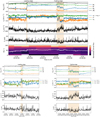 |
Fig. 3 Same as Fig. 1, but for event 2 on November 1, 2018, starting at 23:23:04 UT. The average value of the radial velocity (⟨vR⟩ = 342 km s−1) was removed for easier visualisation. |
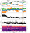 |
Fig. 4 Larger switchback in which event 2 is embedded. The four panels show the same variables as in the first figure of Fig. 3. The sub-structure noted as event 2 is delimited here by two vertical dotted grey bars. |
4 Summary and discussion
In this paper, we report the observation of magnetic reconnection at the boundaries of three magnetic switchbacks observed by PSP. These events were detected during the first encounter of PSP in November 2018. The signatures associated with magnetic reconnection at the switchback boundaries are summarised in Table 1. The main characteristics of these current sheets are listed in Table 2, which namely include the following: magnetic dips, the guide field, magnetic shears, an increase in βp, an increase in the current density and plasma density, the current sheet thickness, distance the to the X-line, and the reconnection jet velocity.
Most of the events that we identified are reconnection exhausts with a significant guide field and a moderate magnetic shear. However, we also identified one event with possible indications of a quasi anti-parallel reconnection (magnetic shear of 168°) with a strong dip in the magnitude of the magnetic field. This suggests that a wide range of reconnection properties may occur at switchback boundaries.
Events 1 and 2 are switchbacks with high guide field magnetic reconnection at both their boundaries. These four current sheets show a typical signature of reconnection exhaust with the following: a correlation and then anti-correlation of the magnetic field and proton velocity in the main direction of the current sheet, and clear proton jets with velocities ranging from 26 to 113% of the respective local Alfvén velocity. It is not uncommon for reconnection jets to be only at a fraction of the Alfvén velocity. There are several explanations for this as detailed in (Phan et al. 2020). These events have a strong guide field as compared to the reconnecting field. Conversely, they have modest dips in the magnitude of the magnetic field (also noted in Phan et al. 2020, and references therein). Finally the angle made by the magnetic field at the two sides of the current sheet is moderate, that is 60° to 80°. Similar characteristics are found at the trailing of event 3, which shows a good indication of reconnection, even though the reconnection jet was not properly resolved.
Event 3 is a switchback with large magnetic field dips of about 90% at both its leading and trailing edges. The trailing edge current sheet shows several pieces of evidence for anti-parallel reconnection. Correlated and anti-correlated variations in the magnetic field and proton velocity upon entry and exit were found, as for the other events. Moreover, the electron strahl was suppressed in this area, indicating a possible disconnection from the Sun. However, the absence of a reconnection jet prevents us from fully concluding on this matter. While the presence of quasi-parallel whistler waves at the boundary of the current sheet, right after the steepest variation in BL (and thus the highest variation in the current) could point to a close approach to the X-line, the distance from the X-line that we computed reveals that the probe was far enough from the X-line to be able to detect such a jet at some point of the crossing. Since reconnection is a 3D process, with only one spacecraft crossing the structure, we may not have totally uncovered its geometrical complexity.
One striking feature of this last event was the large magnetic dips at both boundaries. Farrell et al. (2020) show that switchbacks with magnetic field dips at their boundaries are quite common. As conjectured by these authors, such dips may be created by the diamagnetic currents that are due to the magnetic shear and gradient in density at the boundaries. This has also been noted by Krasnoselskikh et al. (2020). We also evaluate the total current density of j ≃ δB∕(μ0δL) and find comparable values to those reported by Krasnoselskikh et al. (2020) (see Table 1). In the events that we report, the rotation of the magnetic field ranges from 58° to 168° and the current density ranges from 15.2 to 181 nA m−2. It is quite natural that the current density for larger deflections of the magnetic field are stronger. Thus, one can suggest that this type of reconnection mainly occurs across the boundaries of strong magnetic field deflections.
The reconnection events we report were the most striking ones we could find during PSP’s first encounter. So far, they seem to be rare but a more systematic search is needed to quantify their occurrence in the solar wind. On the other hand, magnetic switchbacks seem to occur more frequently in the pristine solar wind. Why they seem more scattered closer to 1 AU has yet to be determined.
The reconnection events we found are all at a distance close to 50 solar radii. We also notice that the velocity increase inside the switchbacks that we analysed is moderate compared to the strong jets that were observed close to the perihelion. On the one hand, we could conjecture that the reconnection at the boundaries destabilise the structure and causes the velocity enhancements to decay. On the other hand, the statistical study of switchbacks near the perihelion presented in Larosa et al. (2021) show that the magnitude of these velocity enhancements is only a few percent of the velocity outside the switchbacks. The velocity enhancements of the structures presented here are consistent with their distribution. However, one could wonder whether strong velocity enhancements would prevent the reconnection for happening at the boundaries of switchbacks. Via simulations, Swisdak et al. (2003) demonstrated that diamagnetic drifts suppress reconnection when the velocity of the moving structure becomes comparable with the Alfvén velocity. They formulated that the reconnection rate would depend on the magnetic shear and on the β. Such parameters would be interesting to explore in future studies.
Overall, one can conjecture that the reconnection process happening at switchback boundaries may contribute to the blending of the structures with the regular wind, through a reconfiguration of the magnetic field, which would eventually dissipate the structures. Magnetic reconnection could erode the switchback boundaries as they travel, mostly affecting strong deflections. Smaller deflections would be less likely to undergo such processes. However, small switchbacks would probably disappear at large distances from the Sun anyway due to the interpenetration of the plasma outside and inside the structures and the restoring force of the magnetic field.
Many more questions arise from these observations. In particular, magnetic reconnection at switchback boundaries could contribute to the local heating of solar wind plasma. However, more investigations, in particular statistical studies, would be needed to evaluate their contribution to the global energetics of the solar wind.
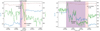 |
Fig. 5 Same as Fig. 2 but for event 2. Correlation and anti-correlation of BL and vL at both boundaries. |
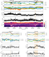 |
Fig. 6 Same as Fig. 1 but for event 3 on November 1, 2018, starting at 18:21:28 UT. The average value of the radial velocity (⟨vR⟩ = 341 km s−1) was removed for easier visualisation. |
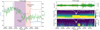 |
Fig. 7 Evidence of reconnection at the trailing edge of event 3. Left panel: follows the same representation as in Fig. 2 but for event 3 and shows a correlation and anti-correlation of BL and vL. Right panels: whistler waves detected right after PSP crossed the current sheet. First panel: SCM waveforms in the RTN coordinates system. Second panel: cross-spectral measurement (trace of the spectral matrix). Third panel: BPF measurements (one component in the SCM sensor frame). For the last two panels, the white lines represent the lower hybrid and electron cyclotron frequencies, respectively. |
Summary of the individual indications for magnetic reconnection.
Characteristics of the reconnection events detected in the current sheets (CS) constituting the switchback boundaries.
Acknowledgements
The authors thank the anonymous referee for their constructive comments. C.F., V.K., T.D., M.K and A.L. acknowledge funding from the CNES. O.A. and V.K. were supported by NASA grant 80NSSC20K0697. O.A. was partially supported by NASA grants 80NNSC19K0848, 80NSSC20K0218, and NSF grant NSF 1914670. S.D.B. acknowledges the support of the Leverhulme Trust Visiting Professorship program. Parker Solar Probe was designed, built, and is now operated by the Johns Hopkins Applied Physics Laboratory as part of NASA’s Living with a Star (LWS) program (contract NNN06AA01C). Support from the LWS management and technical team has played a critical role in the success of the Parker Solar Probe mission. All the data used in this work are available on the public data archive NASA CDAWeb (https://cdaweb.gsfc.nasa.gov/index.html/). Figures were produced using Matplotlib (Hunter 2007).
References
- Agapitov, O. V., Dudok de Wit, T., Mozer, F. S., et al. 2020, ApJ, 891, L20 [Google Scholar]
- Badman, S. T., Bale, S. D., Martínez Oliveros, J. C., et al. 2020, ApJS, 246, 23 [Google Scholar]
- Bale, S. D., Goetz, K., Harvey, P. R., et al. 2016, Space Sci. Rev., 204, 49 [Google Scholar]
- Bale, S. D., Badman, S. T., Bonnell, J. W., et al. 2019, Nature, 576, 237 [Google Scholar]
- Balogh, A., Forsyth, R. J., Lucek, E. A., Horbury, T. S., & Smith, E. J. 1999, Geophys. Res. Lett., 26, 631 [Google Scholar]
- Birn, J., Drake, J. F., Shay, M. A., et al. 2001, J. Geophys. Res. Space Phys., 106, 3715 [Google Scholar]
- Case, A. W., Kasper, J. C., Stevens, M. L., et al. 2020, ApJS, 246, 43 [Google Scholar]
- Cassak, P. A. 2016, Space Weather, 14, 186 [Google Scholar]
- Drake, J. F., Agapitov, O., Swisdak, M., et al. 2021, A&A, 650, A2 (PSP SI) [EDP Sciences] [Google Scholar]
- Dudok de Wit, T., Krasnoselskikh, V. V., Bale, S. D., et al. 2020, ApJS, 246, 39 [Google Scholar]
- Fargette, N., Lavraud, B., Rouillard, A., et al. 2021, A&A, 650, A11 (PSP SI) [EDP Sciences] [Google Scholar]
- Farrell, W. M., MacDowall, R. J., Gruesbeck, J. R., Bale, S. D., & Kasper, J. C. 2020, ApJS, 249, 28 [Google Scholar]
- Fisk, L. A., & Kasper, J. C. 2020, ApJ, 894, L4 [Google Scholar]
- Fox, N. J., Velli, M. C., Bale, S. D., et al. 2016, Space Sci. Rev., 204, 7 [NASA ADS] [CrossRef] [Google Scholar]
- Fujimoto, K., & Sydora, R. D. 2008, Geophys. Res. Lett., 35, 19 [Google Scholar]
- Gosling, J. T., Skoug, R. M., McComas, D. J., & Smith, C. W. 2005, J. Geophys. Res. Space Phys., 110, A1 [Google Scholar]
- Graham, D. B., Vaivads, A., Khotyaintsev, Y. V., & André, M. 2016, J. Geophys. Res. Space Phys., 121, 1934 [Google Scholar]
- He, J., Zhu, X., Yang, L., et al. 2020, ApJ, submitted [arXiv:2009.09254] [Google Scholar]
- Horbury, T. S., Matteini, L., & Stansby, D. 2018, MNRAS, 478, 1980 [Google Scholar]
- Horbury, T. S., Woolley, T., Laker, R., et al. 2020, ApJS, 246, 45 [Google Scholar]
- Huang, S. Y., Yuan, Z. G., Sahraoui, F., et al. 2017, J. Geophys. Res. Space Phys., 122, 7188 [Google Scholar]
- Hunter, J. D. 2007, Comput. Sci. Eng., 9, 90 [NASA ADS] [CrossRef] [Google Scholar]
- Jannet, G., Dudok de Wit, T., Krasnoselskikh, V. V., et al. 2021, J. Geophys. Res., in press [Google Scholar]
- Kasper, J. C., Abiad, R., Austin, G., et al. 2016, Space Sci. Rev., 204, 131 [NASA ADS] [CrossRef] [Google Scholar]
- Kasper, J. C., Bale, S. D., Belcher, J. W., et al. 2019, Nature, 576, 228 [Google Scholar]
- Kim, T. K., Pogorelov, N. V., Arge, C. N., et al. 2020, ApJS, 246, 40 [Google Scholar]
- Krasnoselskikh, V., Larosa, A., Agapitov, O., et al. 2020, ApJ, 893, 93 [Google Scholar]
- Larosa, A., Krasnoselskikh, V., Dudok de Wit, T., et al. 2021, A&A, 650, A3 (PSP SI) [EDP Sciences] [Google Scholar]
- Lavraud, B., Fargette, N., Réville, V., et al. 2020, ApJ, 894, L19 [Google Scholar]
- Liu, Y.-H., Hesse, M., Guo, F., et al. 2017, Phys. Rev. Lett., 118, 085101 [Google Scholar]
- Macneil, A. R., Owens, M. J., Berčič, L., & Finley, A. J. 2020, MNRAS, 498, 5273 [Google Scholar]
- Malaspina, D. M., Ergun, R. E., Bolton, M., et al. 2016, J. Geophys. Res. Space Phys., 121, 5088 [Google Scholar]
- McManus, M. D., Bowen, T. A., Mallet, A., et al. 2020, ApJS, 246, 67 [Google Scholar]
- Mozer, F. S., Agapitov, O. V., Bale, S. D., et al. 2020, ApJS, 246, 68 [Google Scholar]
- ∅ieroset, M., Phan, T. D., Fujimoto, M., Lin, R. P., & Lepping, R. P. 2001, Nature, 412, 414 [Google Scholar]
- Phan, T. D., Bale, S. D., Eastwood, J. P., et al. 2020, ApJS, 246, 34 [Google Scholar]
- Riley, P., Downs, C., Linker, J. A., et al. 2019, ApJ, 874, L15 [Google Scholar]
- Roberts, M. A., Uritsky, V. M., DeVore, C. R., & Karpen, J. T. 2018, ApJ, 866, 14 [Google Scholar]
- Ruffolo, D., Matthaeus, W. H., Chhiber, R., et al. 2020, ApJ, 902, 94 [Google Scholar]
- Santolík, O., Parrot, M., & Lefeuvre, F. 2003, Radio Sci., 38, 1 [Google Scholar]
- Sonnerup, B. U. Ö., & Scheible, M. 1998, ISSI Sci. Rep. Ser., 1, 185 [Google Scholar]
- Squire, J., Chandran, B. D. G., & Meyrand, R. 2020, ApJ, 891, L2 [Google Scholar]
- Sterling, A. C., & Moore, R. L. 2020, ApJ, 896, L18 [Google Scholar]
- Swisdak, M., Rogers, B. N., Drake, J. F., & Shay, M. A. 2003, J. Geophys. Res. Space Phys., 108, A5 [Google Scholar]
- Szabo, A., Larson, D., Whittlesey, P., et al. 2020, ApJS, 246, 47 [Google Scholar]
- Tenerani, A., Velli, M., Matteini, L., et al. 2020a, ApJS, 246, 32 [Google Scholar]
- Tenerani, A., Velli, M., & Matteini, L., et. al. 2020b, AGU Fall meeting 2020, #SH055-04 [Google Scholar]
- Velli, M., Bale, S., & the FIELDS Team on Parker Solar Probe. 2020, AGU Fall meeting 2020, #SH052-03 [Google Scholar]
- Vörös, Z., Yordanova, E., Graham, D. B., Khotyaintsev, Y. V., & Narita, Y. 2019, J. Geophys. Res. Space Phys., 124, 8551 [Google Scholar]
- Wei, X. H., Cao, J. B., Zhou, G. C., et al. 2007, J. Geophys. Res. Space Phys., 112, A10 [Google Scholar]
- Whittlesey, P. L., Larson, D. E., Kasper, J. C., et al. 2020, ApJS, 246, 74 [Google Scholar]
- Woodham, L. D., Horbury, T. S., & Matteini, L. 2021, A&A, 650, L1 (PSP SI) [EDP Sciences] [Google Scholar]
- Zweibel, E. G., & Yamada, M. 2009, ARA&A, 47, 291 [Google Scholar]
- Zweibel, E. G., & Yamada, M. 2016, Proceedings Royal Society A: Mathematical, Physical and Engineering Science, 472, 20160479 [Google Scholar]
All Tables
Characteristics of the reconnection events detected in the current sheets (CS) constituting the switchback boundaries.
All Figures
|
Fig. 1 Event 1 on November 2, 2018, starting at 13:05:09 UT. The shaded areas delimit the boundaries of the switchback, noted as leading and trailing edges. First panel: DC magnetic field measurements from FIELDS/MAG in the RTN frame. Second panel: proton velocity from SWEAP/SPC, also in the RTN frame. The average value of the radial velocity (⟨vR ⟩ = 320 km s−1) was removed for easier visualisation. Third panel: proton density from SWEAP/SPC. Fourth panel: radial proton temperaturefrom SWEAP/SPC. Fifth panel: pitch angle distribution of 314 eV electrons from SWEAP/SPAN-E. The combined flux (two sensors) was normalised by the averaged flux. The white curve represents the magnitude of the magnetic field in arbitrary units. Bottom panels: two sets of plots at the bottom are excerpts of the leading and trailing edges of theswitchback; they represent the same variables (except for the pitch-angle distribution) in the same order. For these two sets of plots, the magnetic field and proton velocity are represented in the local current sheet coordinates LMN. The average value of the velocity for each component was removed for easier visualisation. |
| In the text | |
|
Fig. 2 Correlation and anti-correlation of BL and vL at the boundaries of event 1. The leading edge is represented in the left panel and trailing edge in the right panel. Evolution of BL and vL, component along the main direction of the current sheets. The Pearson correlation coefficients shown were computed in the coloured time windows, chosen to maximise the correlation values. The light brown line is the magnitude of the magnetic field. |
| In the text | |
|
Fig. 3 Same as Fig. 1, but for event 2 on November 1, 2018, starting at 23:23:04 UT. The average value of the radial velocity (⟨vR⟩ = 342 km s−1) was removed for easier visualisation. |
| In the text | |
|
Fig. 4 Larger switchback in which event 2 is embedded. The four panels show the same variables as in the first figure of Fig. 3. The sub-structure noted as event 2 is delimited here by two vertical dotted grey bars. |
| In the text | |
|
Fig. 5 Same as Fig. 2 but for event 2. Correlation and anti-correlation of BL and vL at both boundaries. |
| In the text | |
|
Fig. 6 Same as Fig. 1 but for event 3 on November 1, 2018, starting at 18:21:28 UT. The average value of the radial velocity (⟨vR⟩ = 341 km s−1) was removed for easier visualisation. |
| In the text | |
|
Fig. 7 Evidence of reconnection at the trailing edge of event 3. Left panel: follows the same representation as in Fig. 2 but for event 3 and shows a correlation and anti-correlation of BL and vL. Right panels: whistler waves detected right after PSP crossed the current sheet. First panel: SCM waveforms in the RTN coordinates system. Second panel: cross-spectral measurement (trace of the spectral matrix). Third panel: BPF measurements (one component in the SCM sensor frame). For the last two panels, the white lines represent the lower hybrid and electron cyclotron frequencies, respectively. |
| In the text | |
Current usage metrics show cumulative count of Article Views (full-text article views including HTML views, PDF and ePub downloads, according to the available data) and Abstracts Views on Vision4Press platform.
Data correspond to usage on the plateform after 2015. The current usage metrics is available 48-96 hours after online publication and is updated daily on week days.
Initial download of the metrics may take a while.