| Issue |
A&A
Volume 650, June 2021
Parker Solar Probe: Ushering a new frontier in space exploration
|
|
|---|---|---|
| Article Number | A20 | |
| Number of page(s) | 8 | |
| Section | The Sun and the Heliosphere | |
| DOI | https://doi.org/10.1051/0004-6361/202039639 | |
| Published online | 02 June 2021 | |
Identification of coherent structures in space plasmas: the magnetic helicity–PVI method
1
Dipartimento di Fisica, Università della Calabria,
87036
Cosenza,
Italy
e-mail: This email address is being protected from spambots. You need JavaScript enabled to view it.
2
Department of Physics and Astronomy and Bartol Research Institute, University of Delaware,
Newark,
DE
19716,
USA
e-mail: This email address is being protected from spambots. You need JavaScript enabled to view it.
Received:
9
October
2020
Accepted:
14
November
2020
Abstract
Context. Plasma turbulence can be viewed as a magnetic landscape populated by large- and small-scale coherent structures. In this complex network, large helical magnetic tubes might be separated by small-scale magnetic reconnection events (current sheets). However, the identification of these magnetic structures in a continuous stream of data has always been a challenging task.
Aims. Here, we present a method that is able to characterize both the large- and small-scale structures of the turbulent solar wind, based on the combined use of a filtered magnetic helicity (Hm) and the partial variance of increments (PVI).
Methods. This simple, single-spacecraft technique was first validated via direct numerical simulations of plasma turbulence and then applied to data from the Parker Solar Probe mission.
Results. This novel analysis, combining Hm and PVI methods, reveals that a large number of flux tubes populate the solar wind and continuously merge in contact regions where magnetic reconnection and particle acceleration may occur.
Key words: magnetic fields / magnetohydrodynamics (MHD) / plasmas / turbulence / methods: observational / solar wind
© ESO 2021
1 Introduction
The heliospheric plasma is embedded in a turbulent magnetic field originating from the Sun. Its rotating motion, together with fully developed turbulence, small-scale magnetic reconnection, and wave-like activity produce complex topological structures that propagate away, filling the solar wind (Jokipii 1966; Jokipii & Parker 1969). Of the many types and sizes of magnetic structures that can emerge, perhaps the largest structures are the sporadically occurring magnetic clouds, or interplanetary coronal mass ejections (ICMEs), which may extend more than an AU (Burlaga et al. 1981; Bothmer & Schwenn 1998; Scolini et al. 2019) while having a significant impact on particle propagation and energization. However, magnetic structures may exist over a very wide range of scales and exhibit a diverse morphology and plasma properties (Borovsky 2008). On the other hand, a familiar, and even common, feature of these solar wind structures is the helical winding of magnetic field lines. This class of magnetic structures, such as flux ropes (or flux tubes), are believed to fill a large fraction of the interplanetary volume and might be sites of heating and particle energization (Pecora et al. 2019b). This perspective is often described as a “tangled spaghetti model” and dates back to the earliest models of the interplanetary medium (McCracken & Ness 1966). This interpretation was subsequently extended to view the interplanetary magnetic field as an ensemble of flux tubes, bounded by directional discontinuities (Burlaga 1969). The spaghetti model has been revived and interpreted on a number of more recent occasions (Bruno et al. 2001; Borovsky 2008), including the association of boundaries with tangential and rotational discontinuities (TDs and RDs; Greco et al. 2009). Discontinuities have been described as approximations to trapping boundaries (Tessein et al. 2016; Seripienlert et al. 2010) that can confine energetic particles within flux ropes (Tooprakai et al. 2007; Pecora et al. 2018) or, in the case of a solar moss model, exclude particles from the flux rope cores (Kittinaradorn et al. 2009).
Though their origin still remains uncertain, there is a reasonable consensus that flux ropes, or current carrying flux tubes, can form close to the Sun and propagate outwards, or they can be generated locally by nonlinear interactions in the solar wind, or both. Despite the wide range of scales these structures span, they have peculiar common signatures that are often clearly identifiable. For example, they show a rotation of one magnetic field component, accompanied by large magnetic field magnitude and density lower than the surrounding, ambient solar wind. Furthermore, they tend to assume a cylindrical symmetry of the magnetic field about a central axis. One may generalize this scenario to anticipate a wider variety of adjacent flux tubes (ropes) that have contrasting temperatures, densities, and magnetic field strengths, but with an approximate transverse total pressure balance (Borovsky 2008).
Previous studies used the aforementioned properties to find flux tubes (or flux ropes or filaments) in the solar wind beginning with very detailed approaches that examine a number of parameters (McCracken & Ness 1966; Burlaga 1969; Borovsky 2008). These approaches allow distinctions to be made and for classifications of different types of magnetic flux structures. For example, the magnetic fields can be fitted to a Lundquist model to identify relaxed force-free states in magnetic clouds (Burlaga 1988). Other techniques also enable the identification of other classes of flux tubes or flux ropes. Smaller scale flux ropes, such as “plasmoids” associated with byproducts of magnetic reconnection (Matthaeus & Lamkin 1986), can be implicated in particle energization (Ambrosiano et al. 1988; Drake et al. 2006; Khabarova et al. 2016) and frequently occur in turbulence (Wan et al. 2014). The detection of these structures has been proposed based on cross helicity, residual energy, and magnetic helicity evaluated using a wavelet analysis (Zhao et al. 2020). In the realm of more elaborate techniques, one may also identify flux ropes for special cases that are near-equilibrium and quasi-two-dimensional. Then the reconstruction methods based on Grad-Shafranov (GS) equilibrium (Sonnerup & Guo 1996; Hu & Sonnerup 2002) provide a pathway to visualize a 2D map of the flux tube cross-section. It is important to bear in mind that the application of a technique such as GS reconstruction requires special conditions; in this case, the total pressure must be, at least approximately, a single-valued function of the magnetic potential (Sonnerup et al. 2016; Hu et al. 2018). A “good reconstruction,” and therefore a reasonable detection of a GS flux tube, will be possible only when such auxiliary conditions are fulfilled (Chen et al. 2020).
In the previous work by Pecora et al. (2019a), a GS method was employed in conjunction with the Partial Variance of Increments (PVI) method (Greco et al. 2009) to identify near-equilibrium flux tubes and nearby discontinuities. The clear result is that magnetic discontinuities are often found to populate both peripheral boundaries of GS flux tubes as well as, in some cases, internal boundaries within the flux tubes. In these recent studies, one begins to find verification of the original conjectures that the interplanetary magnetic field consists of filamentary tubes bounded by discontinuities (McCracken & Ness 1966; Burlaga 1969), while recent advances provide much more detail to this picture (Khabarova et al. 2016). At this point, it may be useful to distinguish between identification methods that are more complex and involve specialized assumptions, such as the GS methodologies or fitting to Lundquist states. These more elaborate methods, which one might call reconstruction methods, typically provide more advanced information about the identified structures when they work; however, they do not always work. While reconstruction methods can provide more information, detection methods can be more versatile and easier to implement. Reconstruction methods, such as GS, can also benefit from a preliminary identification step. We focus on this point in the present study.
In the present paper, we employ two complementary methods that characterize both the large- and small-scale coherent structures of the turbulent solar wind, based on a quantitative evaluation of the magnetic helicity (Hm) and a PVI methodbased on the magnetic field. An evaluation of local magnetic helicity employs a novel real-space method that is shown to identify helical flux tubes. In some sense, this approach can be viewed as a simplification and adaptation of the method employed by Zhao et al. (2020). However, instead of passing over discontinuities, we employ the PVI technique to detect them as potential, both internal and external, boundaries of magnetic flux tubes. We exploit the frequently encounteredhelical nature of flux tubes to suggest a relatively straightforward alternative to the assumptions of two-dimensionality and equilibrium conditions that are adopted in Grad-Shafranov methods. We may thus understand the Hm and PVI methods that we employ to provide complementary information. The proposed simple technique identifies a certain classof self-organized magnetic structures, with a minimum of assumptions, and no claim of exhaustive identification.
The paper is organized as follows. In Sect. 2 we present the method based on large-scale filtered magnetic helicity and small-scale gradients. We test the technique in Sect. 3 by using direct numerical simulations of 2.5D compressible magnetohydrodynamics (MHD). In Sect. 4 we apply our technique to space data by analyzing the Parker Solar Probe (PSP) dataset. Finally, in the last section, we present our discussion and conclusions.
2 Local magnetic helicity and PVI methods
The approach is based on the assumption that magnetic flux tubes carry a finite amount of current density along their magnetic axis. These flux ropes are necessarily characterized by helical magnetic field lines near their magnetic axis, as a consequence of Ampere’s law, in a case in which there is a non-null parallel (to the current) magnetic field component. Typically, in simplified representations these structures are treated as 2.5D, with spatial gradients that mainly develop in the 2D plane perpendicular to the electric current density. In addition, a net magnetic field component may lie along the current axis. In envisioning (and simplifying) turbulence as an ensemble of quasi-parallel, large-scale flux tubes, those with the same polarity are often bounded by steep gradients such as small-scale, tangential discontinuities. In anisotropic turbulence, these represent regions of dynamical interactions between adjacent tubes, and they are often observed in simulations (e.g., Matthaeus & Montgomery 1980; Servidio et al. 2009). When present, these boundaries can be readily identified by a method such as the PVI. The novel feature employed here is to exploit the frequently occurring helical flux tubes, via a large-scale analysis method based on the magnetic helicity, in conjunction with a small-scale PVI technique that identifies the reconnecting boundaries of such flux tubes.
2.1 Theory
The starting point is an ideal rugged invariant of MHD turbulence (in the absence of a mean magnetic field), namely the magnetic helicity Hm = ⟨a ⋅b⟩, where a is the magnetic potential associated to field fluctuations b, while ⟨… ⟩ represents an average over a very large volume, or over a whole isolated system (Woltjer 1958; Taylor 1974; Matthaeus & Goldstein 1982). This invariant can also be estimated by single-spacecraft, 1D measurements, as the off-diagonal part of the autocorrelation tensor (Matthaeus et al. 1982):
 (1)
(1)
Here Rjk(γ) = ⟨Bj(r)Bk(r + γ)⟩ is the correlation tensor evaluated at vector spatial lag γ, and the fluctuations are assumed to be well described by spatially homogeneous statistics, up to the second order correlations. The line integral was evaluated along a specified curve, parameterized as γ (s), from a specified origin at γ (s = 0) to infinity. The differential line element along γ is ds = ds dγ(s)∕ds, where s is the scalar displacement along the curve and dγ(s)∕ds is a unit vector tangent to the curve.
While the principle for evaluating fluctuating helicity has become well known, it most often is applied using suitable Fourier transforms to the evaluation of the reduced, one-dimensional magnetic helicity spectrum. Extending the spectral approach, the helicity measurement has also been implemented using wavelet transforms (Farge 1992; Bruno et al. 1999; Telloni et al. 2012; Zhao et al. 2020). The alternative approach, implemented here, is based on the consideration of the real-space formulation (1). This defining equation may be arbitrarily decomposed as

where the integral is now specialized to the case integration path in a fixed direction ê with scalar lag s. The obvious interpretation is that  is the contribution to helicity from structures larger than ℓ, while
  is the contribution to helicity from structures smaller than ℓ. The methodemployed below is the direct evaluation of the special case
 (4)
(4)
where the integral was again calculated in the direction ê with scalar lag s. It is important to emphasize that this approach provides a measurement for the helicity of the fluctuations that have spatial scales less than ℓ, the principle assumption is that the turbulence is spatially homogeneous.
2.2 Implementation
In the usual way, the above mathematical formulation requires a practical interpretation of the ensemble average (usually accomplished by averaging in space or time), which relies on an ergodic theorem (Panchev 1971). Assuming that a single spacecraft measurement is available and that the measurement point is fixed in space, averaging is done in one Cartesian direction, using the Taylor hypothesis (Jokipii 1973). In this familiar approximation, a spatial lag s is inferred by computing a convected distance in a given time lag, assuming no distortion during this time interval. Therefore, with solar wind speed V = Vê, one approximates s = −V τ, where τ is the time lag.
With these assumptions, the magnetic helicity of the fluctuations, and other derived quantities, such as its reduced one-dimensional spectrum, may be derived from interplanetary spacecraft data (Matthaeus & Goldstein 1982). Here we propose a procedure to calculate a local estimate of Eq. (4). To obtain the requisite elements of the correlation matrix at the point x, we averaged the local correlator (symbolically, “ ”) over a region of width w0 centered about x. To avoid effects of large fluctuations at the edges of the investigated data interval, a window was employed to smoothly let the estimates reach zero at the edges, which is a common procedure in correlation analysis (Matthaeus & Goldstein 1982). Specifically, in the first step, the raw helicity was estimated as
![Mathematical equation: \begin{equation*} C(x, l) = \frac{1}{w_0} \int_{x-\frac{w_0}{2}}^{x+\frac{w_0}{2}} \left[b_2(\xi)b_3(\xi+l) -b_3(\xi)b_2(\xi+l)\right] \textrm{d}\xi.\end{equation*}](/articles/aa/full_html/2021/06/aa39639-20/aa39639-20-eq7.png) (5)
(5)
This was followed by windowing the correlation function C(x, l) as
 (6)
(6)
where ![Mathematical equation: $h(l) = \frac{1}{2}\left[ 1 + \cos\left(\frac{2\pi l}{w_0}\right) \right]$](/articles/aa/full_html/2021/06/aa39639-20/aa39639-20-eq9.png) is the Hann window. The interval of local integration w0 is arbitrary, but we typically chose it as an order unity multiple of the scale ℓ, such as w0 = 2ℓ. Hereafter we refer to the quantity computed inEq. (6) as Hm(x, ℓ) or simply Hm when it does not cause confusion. The above formulas convert to the time domain directly by using the Taylor hypothesis.
is the Hann window. The interval of local integration w0 is arbitrary, but we typically chose it as an order unity multiple of the scale ℓ, such as w0 = 2ℓ. Hereafter we refer to the quantity computed inEq. (6) as Hm(x, ℓ) or simply Hm when it does not cause confusion. The above formulas convert to the time domain directly by using the Taylor hypothesis.
To identify the boundaries of a flux rope, we used the PVI (Greco et al. 2008), defined as
 (7)
(7)
where ΔB(s, ℓ) = B(s + ℓ) −B(s) are the increments evaluated at scale ℓ and the averaging operation ⟨… ⟩ was performed over a suitable interval. The function can be computed spatially in simulations or in magnetic field time series by assuming the Taylor hypothesis. The technique has been strongly validated in different conditions (Greco et al. 2018), identifying current sheets that spontaneously form in between magnetic islands in simulations (Greco et al. 2009) and observations (Pecora et al. 2019a). The technique can also detect local reconnection events in the turbulent solar wind (Osman et al. 2014).
Below, we implement a combined procedure that employs both the local real space magnetic helicity analysis and the PVI method. The purpose is to identify flux tubes and their boundaries, with examples given in simulation and spacecraft analysis using the PSP data.
3 Analysis of turbulence simulations
We tested our novel technique by using direct numerical simulations of compressible MHD. We solved the equations in 2.5D, in a square box with a size of 2πL0 and with a resolution of 20482 grid points. All the quantities were normalized to classical Alfvén units. The simulation was performed in the x-y plane and a mean magnetic field B0 = 1 is present along the z axis. The velocity and magnetic field fluctuations have all three Cartesian components. The code, based on a very accurate pseudo-spectral method (Gottlieb & Orszag 1977; Ghosh et al. 1993), as described in Perri et al. (2017), makes use of a logarithmic density. In order to preserve the solenoidal condition of the magnetic field, the algorithm solves equations for the magnetic potential a and parallel variance bz directly, so that the total magnetic field is decomposed as B = Bzẑ + ∇a ×ẑ. Here, Bz = B0 + bz is the out-of-plane magnetic field, where ∇ = (∂∕∂x, ∂∕∂y, 0) is the in-plane gradient. The algorithm has been stabilized via hyperviscous dissipation so as to suppress very small-scale, spurious numerical effects. For these simulations, we used a small, fourth-order hyperviscosity, with coefficients on the order of 10−8. This numerical tool has been extensively used in recent years with applications to space plasma turbulence (Vásconez et al. 2015; Matthaeus et al. 2015; Perri et al. 2017).
The present simulation parameters are in the range of solar wind conditions, with plasma β = 1 and fluctuation amplitude δb∕B0 = 1∕2, where β is the ratio of kinetic to magnetic pressures and δb is the total root mean square (rms) magnetic fluctuation amplitude. The initial fluctuations were chosen with random phases, for both magnetic and velocity fields in a shell of Fourier modes with 3 ≤ |k|≤ 5, where the components of wave vector are in units of 1∕L0. The decaying MHD simulation quickly develops turbulence and small-scale dissipative structures. The magnetic field power spectrum (not shown here) manifests a power-law typical of Kolmogorov turbulence, namely with a scaling of P(k) ∝ k−5∕3. The turbulent pattern is represented in Fig. 1, where we show the 2D contour lines of constant magnetic potential a (black solid lines), which are readily identified with the in-plane projection of the magnetic field lines. The typical features of 2D turbulence are evident, with large-scale coherent structures and narrow, discontinuous contact regions, where one frequently finds that reconnection is occurring (Servidio et al. 2009). In the same figure, we report, as shaded areas, magnetic flux tubes and reconnecting current sheets, which were identified using a cellular automaton (CA) procedure that is described in Servidio et al. (2011). This CA was built on the topological properties of the magnetic potential. In particular, we first identified the critical points (maxima, minima, and X-points), and then the algorithm propagated information away from these critical points, thus identifying the strongest, large-scale islands (starting from the O-points) and the reconnection regions (starting from the X-points). The result of this procedure is a cellularization of turbulence, as is clear from Fig. 1. These islands retain a finite amount of magnetic helicity due to nonzero parallel variances (bz) that are frequently concentrated near the center of flux ropes.
On this magnetic skeleton, we tested our 1D algorithm, based on the combination of the local magnetic helicity in Eqs. (5)–(6) and the PVI in Eq. (7). In order to test the method and to establish a direct comparison between the plasma simulation and the PSP data, we sent a virtual spacecraft through the periodic domain. Its trajectory is represented in Fig. 1 with oblique blue lines, which intersects both large-scale helical structures (cyan) and small-scale discontinuities (orange). In Fig. 2a, we report the turbulent magnetic field, as observed along the virtual satellite trajectory.
The 1D signals are shown over the entire trajectory along the oblique coordinate s, measured in units of L0. In Fig. 2b we show the out-of-plane current jz which is very intermittent, indicating the presence of magnetic discontinuities. To identify these intermittent features by using the magnetic field, interpolated along the virtual trajectory, we computed the PVI signal, as described in Eq. (7). We used very small increment lags, namelyPVI(s, ℓ = λT∕10), where  is the magnetic Taylor microscale. At these lengths, the time series generated by the PVI method becomes a good surrogate for the current density, as is suggested by comparing panel b and panel c of the same figure (for more on this comparison, see Greco et al. 2018).
To complete the analysis, we computed the filtered magnetic helicity as in Eqs. (5)–(6). First, we rotated the magnetic field b from the Cartesian (bx, by, bz) frame to the trajectory coordinates (b1, b2, b3), where b1 is the component along the trajectory direction ê, b3 remains along z, and b2 completes the right-handed frame. Second, from this rotated field, we computed the Hm signal at the (cumulative) scale ℓ = λc∕2, where λc is the correlation length. As can be seen in the lower panel of Fig. 2, there is a net offset between the large helical flux tubes and the PVI peaks.
By using both the surrogate Hm measurement and the PVI signals, we established a threshold-based method in order to identify the most significant events. For the Hm, we identified the events with helicity values larger than one standard deviation of the Hm distribution as strong flux tubes. For the PVI method, we chose a typical threshold of PVI = 2. It has been shown that the probability distribution of the PVI statistic derived from a non-Gaussian turbulent signal strongly deviates from the probability density function of the PVI computed from a Gaussian signal for values of PVI that are greater than about 2. As PVI increases, the recorded “events” are extremely likely to be associated with coherent structures and therefore inconsistent with a signal having random phases (Greco et al. 2018).
The selected peaks are reported for both Hm and PVI in panels c and d of Fig. 2, respectively. At this point, we have a list of selected events, namely the position of the possible flux ropes (peaks of the filtered magnetic helicity signal) and the reconnection events (peaks of the PVI signal). The position of these coherent structures is recorded in the full 2D map in Fig. 1, and one may observe a very good qualitative agreement of these events with the magnetic potential and the CA painting. Magnetic helicity peaks are located well inside helical islands, close to their cores. A few are located outside and coincide with PVI events, indicating the presence of complex structures in between islands, which is possibly due to a reconnection-induced reorganization of magnetic field topology. On the other hand, red stars – the PVI events – are found at the boundaries of magnetic islands. This precise positioning of magnetic helicity and PVI peaks suggests that the core of a magnetic island can be identified, with noteworthy precision, by a magnetic helicity extremum, and its boundaries coincide well with the closest PVI events on either side. The new method is able to identify the strongest helical flux tubes and the more intermittent magnetic structures, which are likely to be reconnection events.
Figure 3 shows a close-up of the relevant quantities measured along the first segment of the synthetic trajectory. From this 1D information, the identification of magnetic islands is rather straightforward: The oscillations of the PVI signal tend to drop in magnitude near an extremum of local Hm, and the boundaries of the islands are well defined by a sharp increase in PVI. Moreover, inside the island cores, it is evident that the total current is smaller in general, but not zero, in view of Ampere’s law. The net magnetic helicity in a flux rope is indicated by a nonzero component of the out-of-plane magnetic field fluctuation bz. It is interesting to notice how well the Hm peaks fall in a PVI-quiet region in between two strong PVI events.
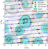 |
Fig. 1 2D line contours of the magnetic potential a (black solid)at the maximum of the turbulent activity of the analyzed MHD simulation. The shaded areas in cyan and orange are magnetic islands and strong current sheets, respectively, as painted by the CA algorithm. The oblique blue lines represent the trajectory of a virtual satellite that sweeps through turbulence. Yellow and green crosses indicate the maxima andminima of the local magnetic helicity, respectively, while red stars are strong PVI events. |
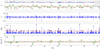 |
Fig. 2 Panel a: magnetic field components and magnitude. Panel b: current density jz in the out-of-plane direction. Panel c: time series of PVI(s, ℓ = λT∕10). Panel d: filtered magnetic helicity evaluated at a correlation scale |
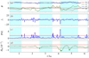 |
Fig. 3 Zoom on magnetic field, current density, PVI, and Hm for the first segment of the trajectory where three peaks of helicity and twelve PVI events have been identified. Shaded cyan and orange areas represent the CA structures reported in Fig. 1. The Hm peaks fall inPVI-quiet regions, in between consecutive, strong PVI clusters. |
4 Analysis of PSP dataset
We applied the Hm–PVI technique to the fluxgate magnetic field data obtained by the PSP FIELDS instrument suite (Bale et al. 2016). In particular, we analyzed the results obtained from the first perihelion (Bale et al. 2019), which will be further discussed in comparison with other identification techniques (Zhao et al. 2020; Chen et al. 2020). The FIELDS magnetic data were resampled from full resolution to 1-s cadence. Moreover, the first encounter data were divided into 8 h-long subsets, so that each contains several correlation times. The correlation time τC, in the spacecraft frame, is about 10−40 min at radial distances of 0.17−0.25 AU (Parashar et al. 2020). We analyzed several such intervals in the first encounter; however, to make close contact with the above mentioned published works (Zhao et al. 2020; Chen et al. 2020), we concentrate below on the following particular interval: 2018 November 13 from 8:00:00 to 16:00:00 UTC. Fig. 4 shows (a) the magnetic field time series in the RTN coordinate system, (b) the PVI computed at 1s lag, and (c) the magnetic helicity evaluated at the scale of one correlation time. In this interval, the average plasma β ~ 1, as reported by (Chhiber et al. 2020; Zhao et al. 2020; Chen et al. 2020).
Figure 5 shows the analysis of two subintervals of the data shown in Fig. 4, specifically from 9:15 to 12:45 (left panels) and from 13:00 to 13:45 (right panels). Each column shows stacked plots of the magnetic field time series, the PVI, and the local magnetic helicity, which were computed with different maximum lags. The largest lag was chosen to be one correlation time τC, while the smallest wast = 1∕3τC. Regions of high helicity are shaded in cyan, while nearby PVI events are in orange, in analogy with the procedure employed in the simulation. Moreover, pairs of PVI events that bound helical regions are also highlighted with dashed vertical lines. It is evident that the Hm time series suggest a multi-scale nature of helical structures. We recall that the helicity diagnostic incorporates contributions from all scales smaller than the maximum lag.
The left panels of Fig. 5 show two helical structures that are bounded by two strong PVI events each (cyan lines for the first event and magenta lines for the second). At scales smaller than one correlation time (panels d and e), the Hm signal shows a fragmentation of the structures, highlighting smaller features within and near the larger helical structure. Moreover, the two identified cores (cyan shaded regions) might be enclosed within a larger helical structure, possibly bounded by the leftmost cyan and rightmost magenta lines. This description is also consistent with the reconstruction performed in Chen et al. (2020), which shows a large island with two inner structures at about the same period. On the other hand, the right panels show a single structure at t∕τC = 1, which is clearly bounded by PVI events in panel h. At smaller scales, t∕τc = 1∕2 (panel i), t∕τc = 1∕3 (panel j), and Hm signals suggest the absence of relevant internal structures, envisioning a “pristine” flux rope.
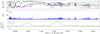 |
Fig. 4 Panel a: PSP FIELDS Fluxgate Magnetometer (MAG) data in RTN coordinates resampled at 1s on 2018 November 13 from 8:30 to 15:30 UTC. In this interval, the correlation time τC ~ 25 min. Panel b: PVI signal and panel c: Hm computed at one correlation time. |
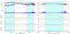 |
Fig. 5 Two close-ups of Fig. 4 from 9:15 to 12:45 (left panels) and from 13:00 to 13:45 (right panels). The figure reports the magnetic field (a) and (f); the PVI signal (b) and (g); and the magnetic helicity evaluated at one correlation time (c), (h), 1∕2 correlation time (d), (i), and 1∕3 of the correlation time (e) and (j). It is interesting to notice that the Hm shape heavily depends on the chosen window, suggesting a multi-scale nature of helical structures. The vertical cyan and magenta lines highlight the position of strong PVI events edging high-helicity regions (cyan shaded regions). Left panels: two structures that are bounded by two strong PVI events each (cyan lines for the first event and magenta lines for the second). At scales smaller than one correlation time, the Hm signal shows a fragmentation of the structure, highlighting sub-features within the helical structure. Moreover, the two identified cores might be enclosed within a larger helical structure, possibly bounded by the leftmost cyan and rightmost magenta lines. This description is also consistent with the reconstruction performed by Chen et al. (2020; their Fig. 4), which shows a large island with two inner structures. On the other hand, the right panels show a smaller structure at t∕τC = 1, clearly bounded by PVI events, which has no internal features. |
5 Discussion
Substantial progress has been made in recent years in identifying magnetic and plasma structures in the solar wind based on the flux tube paradigm (Bruno et al. 2001; Borovsky 2008) and also from the analysis of discontinuities (Neugebauer 2006; Vasquez et al. 2007). Such studies build upon the concept that a substantial volume fraction of the solar wind magnetic field is organized into “filaments” or flux ropes (McCracken & Ness 1966), that is, current carrying flux tubes that maintain their integrity over some reasonable distance. Eventually, due to turbulence, a typical flux tube becomes highly distorted and “shredded” over sufficiently large distances along the magnetic axis (Servidio et al. 2014). The idea that these tubes might act as conduits for solar energetic particles (McCracken & Ness 1966) has recently received theoretical and observational support (Ruffolo et al. 2003; Tessein et al. 2013, 2016; Seripienlert et al. 2010; Tooprakai et al. 2016). Flux rope structures, including smaller secondary “islands,” may also act as sites of particle energization (Ambrosiano et al. 1988; Drake et al. 2006; Khabarova et al. 2016; Malandraki et al. 2019).
The association of discontinuities with flux tube boundaries is often observed in numerical simulations of MHD and plasma turbulence (Matthaeus & Montgomery 1980; Servidio et al. 2010; Haggerty et al. 2017). On the basis of this evidence, it is clear that sharp discontinuities are frequently encountered at peripheral and internal boundaries of flux tubes. However this is not a universal property of flux ropes, and such sharp boundaries are not expected to always be present or to completely envelop flux tubes since they are often the product of the ongoing interaction of adjacent tubes, which may be a time-dependent or even sporadic process.
It is interesting to note that there are at least several types of interesting variations of the relative positioning of helicity peaks and PVI boundaries, as seen in Fig. 1; sometimes there are helicity peaks near the edges of flux tubes. Also, there are sometimes “internal boundaries” in which PVI peaks occur well within flux tubes. Some internal helical structures are also apparent in the PSP data, as seen in panels d and e of Fig. 5, for the helicity computed at scales smaller than a correlation time. The former is reminiscent of nonuniform helicity content in flux tubes envisioned in Taylor’s theory of the dynamical relaxation of flux tubes (Taylor 1986). The latter evokes the internal current structures within flux tubes that are attributed to tokamak disruptions (Kadomtsev 1987, 1984). An investigation of a possible dynamical explanation for the relative positioning between peaks in Hm and PVI as observed here, along with a potential analogy with laboratory plasma dynamical theories, represent interesting directions for future work.
In this paper, we have suggested the cooperative use of two relatively simple methods as an approach to identify flux tubes and coherent current structures that may form at their boundaries. We chose to employ the PVI method for the identification of discontinuities (Greco et al. 2009, 2018) and to use it in conjunction with a real-space method to systematically identify magnetic helicity concentrations, which may be recognized as signatures of helical flux ropes. Neither of these methods provides an absolute identification nor as complete a taxonomy as would be provided by other available methodologies. For example, traditional discontinuity identification methods (Burlaga & Ness 1969; Tsurutani & Smith 1979) and their extensions (Bruno et al. 2001; Neugebauer 2006; Vasquez et al. 2007) allow for more complete classifications of classical MHD and plasma discontinuities. Similarly, various, more complete techniques have been developed for identifying or visualizing the flux ropes themselves (Klein & Burlaga 1982; Borovsky 2008). A particularly elegant class of methods is the Grad-Shafranov reconstruction approach (Hu 2017). The real-space helicity identification approach provides a less complete picture of flux tube structure than these.
The present combination has the advantage of being relatively free of assumptions concerning the types of structures that are being identified. PVI is unbiased concerning discontinuity types, and readily detects TDs, RDs, shocks, etc. Likewise, the only assumption in developing the real space helicity approach is that the statistics of the fluctuations are spatially homogeneous (or, for a time series, time stationary). No assumptions about two-dimensionality or other spatial symmetry are required, in contrast to the standard GS method. In addition, the Hm –PVI identification method has a practical advantage in its simplicity and ease of implementation. We may conclude that the proposed pair of methods have distinct advantages in locating flux ropes and their boundaries in data streams, such as typical single spacecraft solar wind data, as well as in the analysis of very large simulation datasets. This methodology may also prove useful as a first stage of analysis to locate data that are suitable for more elaborate analyses such as Grad-Shafranov reconstruction.
For future work, it will be desirable to carry out statistical surveys of helical flux ropes and their boundaries using the combined Hm –PVI method, which we have described here. There would be considerable scientific value, for example regarding issues of relevance to space weather, in carrying out such surveys at 1AU using extensive datasets such as those available from the ACE and Wind spacecraft. Likewise, surveys of helical flux ropes using additional PSP data as well as Solar Orbiter data (Müller et al. 2020) will be useful in characterizing the magnetic field helical structure of the inner heliosphere, where this information may be of value in understanding the origin of the solar wind. Such surveys may be facilitated using the present approach due to its simplicity of implementation.
Acknowledgements
W.H.M. is partially supported by the Parker Solar Probe mission through the ISOIS Theory and Modeling team and a subcontract from Princeton University (SUB0000317). This project has received funding from the European Unions Horizon 2020 research and innovation program under grant agreement No. 776262 (AIDA, www.aida-space.eu). The PSP data used here is publicly available on NASA CDAWeb https://cdaweb.gsfc.nasa.gov/index.html/.
References
- Ambrosiano, J., Matthaeus, W. H., Goldstein, M. L., & Plante, D. 1988, J. Geophys. Res., 93, 14383 [Google Scholar]
- Bale, S., Goetz, K., Harvey, P., et al. 2016, Space Sci. Rev., 204, 49 [Google Scholar]
- Bale, S. D., Badman, S. T., Bonnell, J. W., et al. 2019, Nature, 576, 237 [Google Scholar]
- Borovsky, J. E. 2008, J. Geophys. Res. Space Phys., 113, A08110 [Google Scholar]
- Bothmer, V., & Schwenn, R. 1998, Ann. Geophys., 16, 1 [Google Scholar]
- Bruno, R., Bavassano, B., Bianchini, L., et al. 1999, Magn. Fields Solar Process., 448, 1147 [Google Scholar]
- Bruno, R., Carbone, V., Veltri, P., Pietropaolo, E., & Bavassano, B. 2001, Planet. Space Sci., 49, 1201 [Google Scholar]
- Burlaga, L. 1988, J. Geophys. Res. Space Phys., 93, 7217 [Google Scholar]
- Burlaga, L. F. 1969, Sol. Phys., 7, 54 [Google Scholar]
- Burlaga, L. F., & Ness, N. F. 1969, Sol. Phys., 9, 467 [Google Scholar]
- Burlaga, L., Sittler, E., Mariani, F., & Schwenn, R. 1981, J. Geophys. Res., 86, 6673 [Google Scholar]
- Chen, Y., Hu, Q., Zhao, L., et al. 2020, ApJ, 903, 76 [Google Scholar]
- Chhiber, R., Goldstein, M. L., Maruca, B. A., et al. 2020, ApJS, 246, 31 [Google Scholar]
- Drake, J. F., Swisdak, M., Che, H., & Shay, M. A. 2006, Nature, 443, 553 [Google Scholar]
- Farge, M. 1992, Ann. Rev. Fluid Mech., 24, 395 [Google Scholar]
- Ghosh, S., Hossain, M., & Matthaeus, W. H. 1993, Comp. Phys. Comm., 74, 18 [Google Scholar]
- Gottlieb, D., & Orszag, S. A. 1977, Numerical Analysis of Spectral Methods: Theory and Applications (SIAM) [Google Scholar]
- Greco, A., Chuychai, P., Matthaeus, W. H., Servidio, S., & Dmitruk, P. 2008, Geophys. Res. Lett., 35, L19111 [Google Scholar]
- Greco, A., Matthaeus, W. H., Servidio, S., Chuychai, P., & Dmitruk, P. 2009, ApJ, 691, L111 [Google Scholar]
- Greco, A., Matthaeus, W., Perri, S., et al. 2018, Space Sci. Rev., 214, 1 [Google Scholar]
- Haggerty, C. C., Parashar, T. N., Matthaeus, W. H., et al. 2017, Phys. Plasmas, 24, 102308 [Google Scholar]
- Hu, Q. 2017, Sci. China Earth Sci., 60, 1466 [Google Scholar]
- Hu, Q., & Sonnerup, B. U. 2002, J. Geophys. Res. Space Phys., 107, [Google Scholar]
- Hu, Q., Zheng, J., Chen, Y., le Roux, J., & Zhao, L. 2018, ApJS, 239, 12 [Google Scholar]
- Jokipii, J. 1966, ApJ, 146, 480 [Google Scholar]
- Jokipii, J. 1973, ARA&A, 11, 1 [Google Scholar]
- Jokipii, J., & Parker, E. 1969, ApJ, 155, 777 [Google Scholar]
- Kadomtsev, B. 1984, Plasma Phys. Control. Fusion, 26, 217 [Google Scholar]
- Kadomtsev, B. 1987, Rep. Prog. Phys., 50, 115 [Google Scholar]
- Khabarova, O. V., Zank, G. P., Li, G., et al. 2016, ApJ, 827, 122 [Google Scholar]
- Kittinaradorn,R., Ruffolo, D., & Matthaeus, W. 2009, ApJ, 702, L138 [Google Scholar]
- Klein, L. W., & Burlaga, L. F. 1982, J. Geophys. Res., 87, 613 [Google Scholar]
- Malandraki, O., Khabarova, O., Bruno, R., et al. 2019, ApJ, 881, 116 [Google Scholar]
- Matthaeus, W. H., & Goldstein, M. L. 1982, J. Geophys. Res., 87, 6011 [Google Scholar]
- Matthaeus, W. H., & Lamkin, S. L. 1986, Phys. Fluids, 29, 2513 [Google Scholar]
- Matthaeus, W. H., & Montgomery, D. 1980, Ann. New York Acad. Sci., 357, 203 [Google Scholar]
- Matthaeus, W. H., Goldstein, M. L., & Smith, C. 1982, Phys. Rev. Lett., 48, 1256 [Google Scholar]
- Matthaeus, W. H., Wan, M., Servidio, S., et al. 2015, Phil. Trans. R. Soc. A Math., Phys. Eng. Sci., 373, 20140154 [Google Scholar]
- McCracken, K., & Ness, N. 1966, J. Geophys. Res., 71, 3315 [Google Scholar]
- Müller, D., St. Cyr, O. C., Zouganelis, I., et al. 2020, A&A, 642, A1 [CrossRef] [EDP Sciences] [Google Scholar]
- Neugebauer, M. 2006, J. Geophys. Res., 111, A04103 [Google Scholar]
- Osman, K., Matthaeus, W., Gosling, J., et al. 2014, Phys. Rev. Lett., 112, 215002 [Google Scholar]
- Panchev, S. 1971, Random Functions and Turbulence (New York: Pergammon Press) [Google Scholar]
- Parashar, T., Goldstein, M., Maruca, B., et al. 2020, ApJS, 246, 58 [Google Scholar]
- Pecora, F., Servidio, S., Greco, A., et al. 2018, J. Plasma Phys., 84, 725840601 [Google Scholar]
- Pecora, F., Greco, A., Hu, Q., et al. 2019a, ApJ, 881, L11 [Google Scholar]
- Pecora, F., Pucci, F., Lapenta, G., Burgess, D., & Servidio, S. 2019b, Sol. Phys., 294, 114 [Google Scholar]
- Perri, S., Servidio, S., Vaivads, A., & Valentini, F. 2017, ApJS, 231, 4 [Google Scholar]
- Ruffolo, D., Matthaeus, W. H., & Chuychai, P. 2003, ApJ, 597, L169 [Google Scholar]
- Scolini, C., Rodriguez, L., Mierla, M., Pomoell, J., & Poedts, S. 2019, A&A, 626, A122 [CrossRef] [EDP Sciences] [Google Scholar]
- Seripienlert, A., Ruffolo, D., Matthaeus, W., & Chuychai, P. 2010, ApJ, 711, 980 [Google Scholar]
- Servidio, S., Matthaeus, W. H., Shay, M. A., Cassak, P. A., & Dmitruk, P. 2009, Phys. Rev. Lett., 102, 115003 [Google Scholar]
- Servidio, S., Matthaeus, W. H., Shay, M. A., et al. 2010, Phys. Plasmas, 17 [Google Scholar]
- Servidio, S., Greco, A., Matthaeus, W. H., Osman, K. T., & Dmitruk, P. 2011, J. Geophys. Res. Space Phys., 116, A09102 [Google Scholar]
- Servidio, S., Matthaeus, W. H., Wan, M., et al. 2014, ApJ, 785, 56 [Google Scholar]
- Sonnerup, B. U. Ö., & Guo, M. 1996, Geophys. Res. Lett., 23, 3679 [Google Scholar]
- Sonnerup, B. U. Ö., Hasegawa, H., Denton, R. E., & Nakamura, T. K. M. 2016, J. Geophys. Res. Space Phys., 121, 4279 [Google Scholar]
- Taylor, J. B. 1974, Phys. Rev. Lett., 33, 1139 [NASA ADS] [CrossRef] [Google Scholar]
- Taylor, J. 1986, Rev. Mod. Phys., 58, 741 [Google Scholar]
- Telloni, D., Bruno, R., D’Amicis, R., Pietropaolo, E., & Carbone, V. 2012, ApJ, 751, 19 [Google Scholar]
- Tessein, J. A., Matthaeus, W. H., Wan, M., et al. 2013, ApJ, 776, L8 [Google Scholar]
- Tessein, J. A., Ruffolo, D., Matthaeus, W. H., & Wan, M. 2016, Geophys. Res. Lett., 43, 3620 [Google Scholar]
- Tooprakai, P., Chuychai, P., Minnie, J., et al. 2007, Geophys. Res. Lett., 34, 17 [Google Scholar]
- Tooprakai, P., Seripienlert, A., Ruffolo, D., Chuychai, P., & Matthaeus, W. 2016, ApJ, 831, 195 [Google Scholar]
- Tsurutani, B. T., & Smith, E. J. 1979, J. Geophys. Res., 84, 2773 [Google Scholar]
- Vásconez, C. L., Pucci, F., Valentini, F., et al. 2015, ApJ, 815, 7 [Google Scholar]
- Vasquez, B. J., Abramenko, V. I., Haggerty, D. K., & Smith, C. W. 2007, J. Geophys. Res., 112, A11102 [Google Scholar]
- Wan, M., Rappazzo, A. F., Matthaeus, W. H., Servidio, S., & Oughton, S. 2014, ApJ, 797, 63 [Google Scholar]
- Woltjer, L. 1958, Proc. Natl. Acad. Sci. USA, 44, 489 [Google Scholar]
- Zhao, L.-L., Zank, G., Adhikari, L., et al. 2020, ApJS, 246, 26 [Google Scholar]
All Figures
|
Fig. 1 2D line contours of the magnetic potential a (black solid)at the maximum of the turbulent activity of the analyzed MHD simulation. The shaded areas in cyan and orange are magnetic islands and strong current sheets, respectively, as painted by the CA algorithm. The oblique blue lines represent the trajectory of a virtual satellite that sweeps through turbulence. Yellow and green crosses indicate the maxima andminima of the local magnetic helicity, respectively, while red stars are strong PVI events. |
| In the text | |
|
Fig. 2 Panel a: magnetic field components and magnitude. Panel b: current density jz in the out-of-plane direction. Panel c: time series of PVI(s, ℓ = λT∕10). Panel d: filtered magnetic helicity evaluated at a correlation scale |
| In the text | |
|
Fig. 3 Zoom on magnetic field, current density, PVI, and Hm for the first segment of the trajectory where three peaks of helicity and twelve PVI events have been identified. Shaded cyan and orange areas represent the CA structures reported in Fig. 1. The Hm peaks fall inPVI-quiet regions, in between consecutive, strong PVI clusters. |
| In the text | |
|
Fig. 4 Panel a: PSP FIELDS Fluxgate Magnetometer (MAG) data in RTN coordinates resampled at 1s on 2018 November 13 from 8:30 to 15:30 UTC. In this interval, the correlation time τC ~ 25 min. Panel b: PVI signal and panel c: Hm computed at one correlation time. |
| In the text | |
|
Fig. 5 Two close-ups of Fig. 4 from 9:15 to 12:45 (left panels) and from 13:00 to 13:45 (right panels). The figure reports the magnetic field (a) and (f); the PVI signal (b) and (g); and the magnetic helicity evaluated at one correlation time (c), (h), 1∕2 correlation time (d), (i), and 1∕3 of the correlation time (e) and (j). It is interesting to notice that the Hm shape heavily depends on the chosen window, suggesting a multi-scale nature of helical structures. The vertical cyan and magenta lines highlight the position of strong PVI events edging high-helicity regions (cyan shaded regions). Left panels: two structures that are bounded by two strong PVI events each (cyan lines for the first event and magenta lines for the second). At scales smaller than one correlation time, the Hm signal shows a fragmentation of the structure, highlighting sub-features within the helical structure. Moreover, the two identified cores might be enclosed within a larger helical structure, possibly bounded by the leftmost cyan and rightmost magenta lines. This description is also consistent with the reconstruction performed by Chen et al. (2020; their Fig. 4), which shows a large island with two inner structures. On the other hand, the right panels show a smaller structure at t∕τC = 1, clearly bounded by PVI events, which has no internal features. |
| In the text | |
Current usage metrics show cumulative count of Article Views (full-text article views including HTML views, PDF and ePub downloads, according to the available data) and Abstracts Views on Vision4Press platform.
Data correspond to usage on the plateform after 2015. The current usage metrics is available 48-96 hours after online publication and is updated daily on week days.
Initial download of the metrics may take a while.