| Issue |
A&A
Volume 649, May 2021
|
|
|---|---|---|
| Article Number | A178 | |
| Number of page(s) | 8 | |
| Section | Galactic structure, stellar clusters and populations | |
| DOI | https://doi.org/10.1051/0004-6361/202140911 | |
| Published online | 01 June 2021 | |
Age and helium content of the open cluster NGC 6791 from multiple eclipsing binary members
III. Constraints from a subgiant⋆
1
Stellar Astrophysics Centre, Department of Physics and Astronomy, Aarhus University, Ny Munkegade 120, 8000 Aarhus C, Denmark
e-mail: This email address is being protected from spambots. You need JavaScript enabled to view it.
2
Astronomical Observatory, Institute of Theoretical Physics and Astronomy, Vilnius University, Saulėtekio av. 3, 10257 Vilnius, Lithuania
3
Department of Astronomy, San Diego State University, San Diego, CA 92182, USA
4
European Southern Observatory, Alonso de Córdova 3107, Vitacura, Santiago, Chile
5
Department of Physics and Astronomy, Aarhus University, Ny Munkegade 120, 8000 Aarhus C, Denmark
6
Department of Astronomy, University of Wisconsin-Madison, Madison, WI 53706, USA
7
Center for Interdisciplinary Exploration and Research in Astrophysics (CIERA) and Department of Physics and Astronomy, Northwestern University, 1800 Sherman Avenue, Evanston, IL 60201, USA
8
Adler Planetarium, Department of Astronomy, 1300 South Lake Shore Drive, Chicago, IL 60605, USA
9
Department of Astronomy and Theoretical Physics, Lund Observatory, Lund University, Box 43 221 00 Lund, Sweden
10
School of Physics, University of New South Wales, NSW 2052, Australia
11
Sydney Institute for Astronomy (SIfA), School of Physics, University of Sydney, NSW 2006, Australia
12
Harvard-Smithsonian Center for Astrophysics, Cambridge, MA 02138, USA
13
Department of Physics and Astronomy, Johns Hopkins University, 3400 North Charles Street, Baltimore, MD 21218, USA
Received:
29
March
2021
Accepted:
25
April
2021
Abstract
Context. Models of stellar structure and evolution can be constrained using accurate measurements of the parameters of eclipsing binary members of open clusters. Multiple binary stars provide the means to tighten the constraints and, in turn, to improve the precision and accuracy of the age estimate of the host cluster. In the previous two papers of this series, we have demonstrated the use of measurements of multiple eclipsing binaries in the old open cluster NGC 6791 to set tighter constraints on the properties of stellar models than was previously possible, thereby improving both the accuracy and precision of the cluster age.
Aims. We identify and measure the properties of a non-eclipsing cluster member, V56, in NGC 6791 and demonstrate how this provides additional model constraints that support and strengthen our previous findings.
Methods. We analyse multi-epoch spectra of V56 from FLAMES in conjunction with the existing photometry and measurements of eclipsing binaries in NGC6971.
Results. The parameters of the V56 components are found to be Mp = 1.103 ± 0.008 M⊙ and Ms = 0.974 ± 0.007 M⊙, Rp = 1.764 ± 0.099 R⊙ and Rs = 1.045 ± 0.057 R⊙, Teff,p = 5447 ± 125 K and Teff,s = 5552 ± 125 K, and surface [Fe/H] = +0.29 ± 0.06 assuming that they have the same abundance.
Conclusions. The derived properties strengthen our previous best estimate of the cluster age of 8.3 ± 0.3 Gyr and the mass of stars on the lower red giant branch (RGB), which is MRGB = 1.15 ± 0.02 M⊙ for NGC 6791. These numbers therefore continue to serve as verification points for other methods of age and mass measures, such as asteroseismology.
Key words: binaries: spectroscopic / stars: fundamental parameters / stars: individual: V604 Lyr / stars: abundances / open clusters and associations: individual: NGC6791
Tables A.1 and A.2 are only available at the CDS via anonymous ftp to cdsarc.u-strasbg.fr (130.79.128.5) or via http://cdsarc.u-strasbg.fr/viz-bin/cat/J/A+A/649/A178
© ESO 2021
1. Introduction
Star clusters allow age estimates of their stars from various ways of isochrone fitting to their photometric colour-magnitude diagram (CMD). If the cluster hosts eclipsing binary stars close to the turn-off, they can improve the age measurements because they provide direct measurements of mass and radius at age sensitive locations in the CMD. This has been exploited in both globular clusters (e.g., Brogaard et al. 2017; Kaluzny et al. 2014, 2015; Thompson et al. 2010, 2020) and open clusters (e.g., Brogaard et al. 2011; Kaluzny et al. 2006; Knudstrup et al. 2020; Meibom et al. 2009; Sandquist et al. 2016; Torres et al. 2020). However, sometimes the eclipsing systems found are on the main sequence, which still allows some model constraints, but not on the age (e.g., Brogaard et al. 2021).
The properties of the old open cluster NGC 6791 were examined in detail by Brogaard et al. (2011, 2012), who exploited the presence of two eclipsing systems, V18 and V20, at the cluster turn-off for a strong age constraint. Here, we demonstrate how a non-eclipsing spectroscopic binary can also allow a strong age constraint when present in a cluster with less evolved eclipsing systems.
V604 Lyr, also known as V56 (Mochejska et al. 2002) and V96 (Bruntt et al. 2003) (RA 19:20:45.26, Dec +37:45:48.6; Gaia Collaboration 2018), is a photometric variable located slightly above the sub-giant branch (SGB) in the CMD of NGC 6791, and we observed it with FLAMES at the Very Large Telescope for this reason. In this paper, we use the name V56, which we found to be a non-eclipsing SB2 binary with an orbital period of 10.822 days. Because of the location in an open cluster with well-measured eclipsing binaries (Brogaard et al. 2011, 2012), precise parameters of the sub-giant component of V56 can be extracted and used for constraining the cluster age, which is the aim of this paper.
In Sect. 2 we describe our spectroscopic observations. Section 3 explains how we extracted multi-epoch radial velocities of V56, the derivation of the spectroscopic orbit, and the determination of masses, effective temperatures, and radii through exploitation of the cluster CMD and the known properties of the eclipsing binaries V18 and V20 (Brogaard et al. 2011, 2012). We discuss the results in the context of the age of NGC6791 in Sect. 4 and summarise our conclusions in Sect. 5.
2. Observations
We obtained spectra for a number of interesting stars in NGC 6791 from FLAMES (Pasquini et al. 2000) at the Very Large Telescope using the GIRAFFE spectrograph in Medusa mode (ESO programme ID 091.D-0125, PI: K. Brogaard). V56 was chosen as a target because it was a known photometric variable (Mochejska et al. 2002; Bruntt et al. 2003), although it was not known to be a binary prior to our observations. With the HR10 setting (533.9 nm–561.9 nm, central wavelength 548.8 nm), the spectral resolution is R = 19 800, corresponding to 15.15 km s−1. We obtained 13 epochs of spectra, 11 with exposure times of 5400 s, the last two with an exposure time of 4800 s. The spectra were reduced using the standard instrument pipeline. For each target spectrum, a mean sky background from a number of sky fibres was subtracted. Thorium-Argon (ThAr) wavelength calibration frames were not obtained during the nights of observation because the simultaneous ThAr option was disabled to avoid contamination in the spectra of the faint targets. Therefore, we applied radial velocity zero-point corrections to the spectra calibrated with standard day-time calibration frames. These corrections were calculated from changes in the nightly mean radial velocity of brighter giant stars that were also observed, as detailed in Brogaard et al. (2018a). After this procedure, the radial velocity epoch-to-epoch root mean square and half-range for single red giant branch members drop significantly from just above 0.5 km s−1 for both numbers to about 0.15 and 0.2 km s−1, respectively. We therefore estimate that the absolute uncertainty of the radial velocity zero-point of each observation is about 0.2 km s−1.
3. Parameters of V56
We used the spectral information in combination with information and observations from our study of eclipsing binaries in NGC 6791 to determine the properties of V56 as detailed in this section.
3.1. Radial velocity measurements
For V56 we measured spectroscopic radial velocities (RVs) and a spectroscopic light ratio from the full available wavelength range in the single Giraffe order. This was done using a combination of the broadening function (BF) formalism (Rucinski 2002) and spectral separation (González & Levato 2006). Spectral lines from two components are visible in 12 epochs of the spectra making V56 a SB2 system. One epoch showed very significant RV overlap between components to a level that high precision RVs could not be extracted, even when using spectral separation. This spectrum was therefore left out of the analysis. The measured RVs are given in Table 1. The uncertainties were first estimated by comparing RVs derived from the full spectral range to RVs derived from each half of the full range. This indicated uncertainties of the order 0.2 km s−1. However, to account for the RV zero-point uncertainty as well (cf. Sect. 2), we adopted total uncertainties of 0.3 km s−1, which is implied both by adding the two error contributions in quadrature, and the χ2 of our orbit solution, see Sect. 3.2. Table 2 shows all our measurements of V56 based on the RVs and additional observations as presented in the following subsections.
Radial velocity measurements of V56.
3.2. Spectroscopic orbit
We calculated orbit solutions of V56 with the RVs in Table 1 using a Python implementation of the programme SBOP (Etzel 2004) created by one of us (J. Jessen-Hansen). When fitting the radial velocities, we allowed the systemic velocity of each component to vary independently because the components and their analysis could be affected differently by gravitational redshift and convective blueshift (Gray 2009) effects. As would be expected for a smaller and less evolved star from both effects, the derived values show that the secondary has a slightly more redshifted system velocity. Uncertainties on the derived system velocities are however too large to allow a meaningful detailed analysis of these physical effects. A solution forcing a common system velocity was also tried. That solution had systemic velocity γ = −46.71, slightly reduced semi-amplitudes, and thus smaller minimum masses by much less than 1σ. The system velocity is fully consistent with cluster membership, since the mean cluster RV is −47.40 ± 0.13 km s−1 with a 1σ velocity dispersion of 1.1 ± 0.1 km s−1 according to Tofflemire et al. (2014).
The first solutions had eccentricity and argument of periastron as free parameters, but converged near zero eccentricity. Solutions with two system velocities had e < 10−4 with an uncertainty larger than the eccentricity itself. When forcing one common system velocity we found e = 0.0047 ± 0.0016. This indicates that our measurements are not precise enough to either rule out or confirm a small eccentricity at a level of 5 ⋅ 10−3 or less. V56 would be expected to have circularised at the age of the cluster, as evidenced by the circularisation period in the similarly old open cluster NGC 188 being 14.5 days according to Meibom & Mathieu (2005), and by comparing to the eclipsing binary V20 in NGC 6791 which has a circular orbit with an orbital period of 14.47 days (Brogaard et al. 2011). However, the circularisation time scale is expected to be much longer than the synchronisation time scale, and we find indications in Sect. 3.5 that V56 is not synchronised, so perhaps it is not circularised either. Whether true or not, we chose to fix the orbital solution to zero eccentricity, after verifying that this has negligible impact on the other parameters, especially the mass ratio q, which is the important number for reaching the absolute mass of the primary component of V56.
The uncertainties in Table 1 were estimated by increasing the systematic uncertainty from the radial velocity zero-point until our orbit solution returned a χ2 of 1.0. The small increase needed of only 0.1 km s−1 suggests that the main uncertainty contribution is the RV zero-points, and thus all epochs and both components were estimated to have the same total uncertainty of 0.3 km s−1.
Figure 1 shows the orbit solution and Table 2 displays the adopted spectroscopic parameters of V56, including the minimum masses. To obtain realistic uncertainties for the minimum masses, we recalculated the orbit as many times as we have epochs of observations, each time shifting the O–C pattern and recalculating. We estimated the uncertainty on the minimum masses from the minimum and maximum values obtained from these 12 solutions. The corresponding uncertainties for the semi-amplitudes are slightly larger than the uncertainty given by the adopted solution.
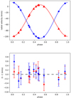 |
Fig. 1. Upper panel: SB2 orbit solution for V56. Red triangles are the RV measurements of the primary component and blue circles are the RV measurements of the secondary. Lower panel: O–C diagram of the RV measurements relative to the model in the top panel. |
Parameters of V56.
3.3. Light ratio
The light ratio, Ls/Lp = 0.386 ± 0.020, was determined as the ratio of the areas under the BF peaks of the separated spectra, calculated using separate templates (Coelho et al. 2005) for each component with parameters selected by comparison to the eclipsing binary member V18 (Brogaard et al. 2011, 2012) in the CMD. The uncertainty of ±0.020, which is conservatively chosen to accommodate both random epoch-to-epoch scatter and a potential systematic bias due to differences in effective temperatures and log g between components, was estimated by comparing to alternative, but less accurate, approaches: Using identical templates for both components resulted in Ls/Lp = 0.399. When calculating the light ratio directly in the observed spectra, using the procedure explained by Kaluzny et al. (2006), which does not take into account the Teff and log g differences between components, we got Ls/Lp = 0.41 ± 0.006, where the uncertainty is the standard deviation of the mean of individual epoch results.
3.4. Masses
We measured the masses of the V56 components by combining the orbital solution with information from the cluster CMD and previous measurements of the eclipsing binary members V18 and V20 (Brogaard et al. 2011, 2012). By requiring that both components of V56 are located on the cluster fiducial sequence, as defined by a polynomial fit to the observed CMD, we found potential CMD positions for the individual components. These positions, shown by the blue line-segments in Fig. 2, were further constrained by making use of the light ratio Ls/Lp = 0.386 ± 0.020 as calculated earlier from the spectra, cf. Sect. 3.3. Adopting this light ratio constrained the V magnitudes to regions marked by the red lines in Fig. 2, and the best estimate of the CMD position of each component were chosen as the intersect of the red and blue line-segments. Since we know the mass at close-by locations on the CMD sequence from the components of the eclipsing member V18 (marked by green circles in Fig. 2), we could interpolate linearly in mass along the sequence to obtain the mass at the position of the secondary of V56. We performed tests using isochrones to verify that linear interpolation in mass versus V-mag over the relevant interval is precise to a level of 0.0002 M⊙. By comparing this mass of the V56 secondary to the minimum mass and the mass ratio found from the spectroscopic orbit, we obtained the orbit inclination and the mass of the primary component, which is on the subgiant branch. The masses of V56 calculated in this way turn out to be 1.103 ± 0.006 M⊙ and 0.974 ± 0.006 M⊙ for the primary and secondary components, respectively. To these uncertainties, we add for both stars in quadrature the contribution from the uncertainty on the masses of the V18 components, ±0.0033 M⊙ (Brogaard et al. 2012). The uncertainty on the V56 primary mass includes the additional error contribution from the uncertainty on the mass ratio q of V56 from the orbit solution, which amounts to ±0.0040 M⊙, which was also added in quadrature. Including all the error contributions, our mass estimates for V56 are Mp = 1.103 ± 0.008 M⊙ and Ms = 0.974 ± 0.007 M⊙.
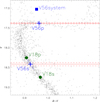 |
Fig. 2. V56 in the CMD of NGC6791. Grey dots are the photometry of NGC 6791 from Brogaard et al. (2012). The blue square represents the total light of V56. The blue line segments correspond to a range of pairs of V56 component magnitudes that combine to the total light magnitude while having one component on the cluster main sequence. The solid red lines give the V56 component V-band magnitudes as calculated from the total light magnitude and the spectroscopic light ratio. Dashed red lines are the corresponding 1σ uncertainties. Blue crosses are the best estimate V56 component magnitudes from the combined constraints of the cluster sequence and the spectroscopic light ratio. Green circles are the V18 component magnitudes. |
3.5. Photometric variability
Since V56 is a known photometric variable but of unknown type, we investigated the Kepler light curve that we extracted from the so-called superstamps of NGC 6791 (Kuehn et al. 2015). We downloaded the superstamps for all 17 quarters from MAST. For each quarter we created a one-pixel mask at the coordinate location of V56 to obtain single-pixel light curves using the Python program Lightkurve (Lightkurve Collaboration 2018). Quarters 1, 10, and 13 did not produce meaningful light curves due to bad pixels and/or contaminating neighbouring stars. From the other light curves we created phase plots adjusting the period manually to obtain the smallest scatter by eye. The periods so obtained are shown in Fig. 3 and the weighted mean of these is 11.93 ± 0.02 days. Alternatively, we also determined the period using the periodogram function in Lightkurve, which resulted in a mean period of 12.26 days. The light curves for selected individual quarters are shown in Fig. 4. The photometric period is clearly different from the orbital period, and the amplitude and shape of the variability changes with time. We therefore attribute the variability to spots. The difference between the orbital period, 10.82 days, and the photometric period, 11.93 days, will then have to be attributed to a combination of differential rotation, spot evolution and potential lack of synchronisation. The robustness of the photometric period over long time scales and the relatively large difference between orbit and photometric period seem to suggest the orbit has not synchronised. This is at odds with theory. According to Zahn (1977), synchronisation should happen much faster than circularisation, and in the case of V56 the time scale tsync is less than 0.2 Gyr. Thus something seems to be, or to have been, disturbing V56 and preventing synchronisation.
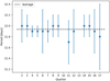 |
Fig. 3. Photometric periods of individual Kepler quarters determined by-eye. Weighted average is 11.93 ± 0.02 days. |
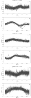 |
Fig. 4. Kepler light curves of V56 for selected quarters folded with the best estimate of the photometric period. |
As in the ground based light curves by Bruntt et al. (2003) where the star has ID V96 the peak-to-peak variability amplitude never exceeds 0.024 mag, except for observational uncertainty and outliers. Since the ground based B and V magnitudes are calculated as the mean of many measurements taken on many different nights we estimate the maximal error in the mean magnitude and B − V colour of V56 is 0.01 mag. We checked that such a change is inconsequential for our conclusions regarding the mass estimates which remain well within the stated uncertainties (changes are of the order ±0.002 M⊙ or less), but the exact colour-location of the primary component on the sub-giant branch can be different by as much as ±0.015 mag in B − V colour. Potential differential reddening effects (Platais et al. 2011; Brogaard et al. 2012) would also cause effects of this order of magnitude. We therefore conclude that we are able to predict the masses of the components of V56 with a precision better than 1% but that the exact CMD position of the sub-giant component has a colour-uncertainty in B − V of about ±0.02 mag.
3.6. Teff
The CMD positions of the V56 components obtained above yields also the component (B − V) colours that can lead to Teff through a colour-Teff relation. To minimise the effect of uncertainty in the reddening, we adjusted E(B − V) in the bolometric correction calculations of Casagrande & VandenBerg (2014) until the colours of the components of V18 were matched at their spectroscopic Teff values by Brogaard et al. (2012). We then used this E(B − V) value to obtain the Teff values corresponding to the colours of the V56 components. This yielded Teff,p = 5447 ± 125 K and Teff,s = 5552 ± 125 K, with the uncertainties conservatively adopted from the largest of the uncertainties on the spectroscopic Teff values for the V18 components. We adopted [Fe/H] = + 0.35 (Brogaard et al. 2012), but using instead [Fe/H] = + 0.29 caused changes of only a few K because it is a relative measurement.
3.7. Radii
The spectral resolution of our observations was R = 19800, corresponding to 15 km s−1. The expected rotational velocities vsin(i) of V56 are significantly smaller. This made us unable to calculate the component radii from vsin(i) measurements as done for the much faster rotating V106 by Brogaard et al. (2018a, their Eq. (1)). Our V56 radii determined as explained below predict vsin(i) values of 6.8–7.5 km s−1 and 4.0–4.5 km s−1 for the primary and secondary, respectively, depending on whether the orbit period or the photometric period (cf. Sect. 3.5) is adopted. Because these are only a fraction of the spectral resolution, and because the spectral lines are further broadened an additional 1–2 km s−1 by the change in radial velocities during the 5400 s long exposures, we were not able to measure meaningful vsin(i) values for V56. Instead, we adopted the below procedure to estimate the radii of the V56 components.
We first used Eq. (10) of Torres (2010) to calculate the absolute component magnitudes:
 (1)
(1)
Here, V⊙ = −26.76 as recommended by Torres (2010) and BCV, ⊙ = −0.068 as obtained from the calibration of Casagrande & VandenBerg (2014), which was also used to obtain the bolometric corrections.
We then combined Eq. (1) with  , σ being the Stefan-Boltzmann constant, and the apparent distance modulus to calculate the radius:
 (2)
(2)
The V-band was utilised because for this filter we have both a spectroscopic light ratio for V56 and a measurement of the apparent distance modulus (V − MV) = 13.51 from Brogaard et al. (2012). With these, Eq. (2) yields Rp = 1.764 ± 0.099 R⊙ and Rs = 1.045 ± 0.057 R⊙. We adopted a 125 K uncertainty on Teff with corresponding bolometric corrections assuming [Fe/H] = + 0.35. An additional error contribution of ±0.005 R⊙ for the primary and ±0.002 R⊙ arises from a change in [Fe/H] of ±0.06. If V18 and V56 are not affected in the same way by small scale differential reddening (Platais et al. 2011; Brogaard et al. 2012) that might add an additional small effect. We have not considered an uncertainty on the apparent distance modulus because this number comes from the analysis of V18 (and V20), and is therefore strongly correlated with the effective temperatures for V18, which are already the sources for our adopted Teff uncertainties.
3.8. Atmospheric parameters
We carried out a classical equivalent-width spectral analysis on the disentangled spectra to determine Teff and [Fe/H] for the two components following the method outlined in Slumstrup et al. (2019). We fixed log g to the values from the binary solution, which are 3.99 and 4.39 for the primary and secondary, respectively. This was determined using the masses and radii from Table 2 with log g = log(GM/R2) in solar units. The atmospheric parameters were determined with the auxiliary program Abundance with SPECTRUM (Gray & Corbally 1994) assuming LTE, using MARCS stellar atmosphere models (Gustafsson et al. 2008) and solar abundances from Grevesse et al. (2007). This yielded Teff = 5490 ± 150 K, [Fe/H] = 0.28 ± 0.07 for the primary and Teff = 5550 ± 190 K, [Fe/H] = 0.34 ± 0.10 for the secondary. The uncertainties are only internal and do not include systematic effects. We show the renormalised disentangled spectra and the corresponding best matching theoretical spectra in Fig. 51.
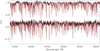 |
Fig. 5. Disentangled and renormalised spectra of the V56 components, primary on top, secondary below. The flux level of the secondary spectrum has been shifted from by −0.8 from 1 for clarity. The observed spectra are shown in black, the model spectra from Sect. 3.8 are overplotted in red. |
Comparison of these Teff values to those derived from photometry in Sect. 3.6 show excellent agreement with differences of only 43 K and 2 K for the primary and secondary, respectively, much less than the 1σ uncertainties. The [Fe/H] values derived are also in excellent agreement with those of Brogaard et al. (2011). The self-consistency of both Teff and [Fe/H] values provide further support for our procedure and derived parameters. We adopt the weighted mean of [Fe/H] of the two V56 components, +0.29 ± 0.06, as the metallicity of V56 in Table 2 while noting that this does not include any systematic uncertainty, and that this is the atmospheric abundance.
4. Results and discussion
We show our measurements in Fig. 6, which is a reproduction of Fig. 4 from Brogaard et al. (2012), now expanded to include V56 in the mass-radius and mass-Teff diagrams. As seen from the mass-radius diagram, the measurements of V56 are consistent within 1σ with the best solution found from V18 and V20. Unsurprisingly, the secondary component of V56 does not constrain the isochrones additionally, because its properties were inferred from the very similar stars in V18 that bracket the V56 secondary. The primary component is however significantly more evolved than any of the other stars in the mass-radius diagram, and therefore provides constraints for the isochrones. The larger measurement uncertainties compared to the eclipsing systems are partly compensated by larger differences between the isochrones at the larger mass corresponding to more evolved stars. The exact best estimate values for mass and radius of the V56 primary suggest an age older by only 0.4 Gyr compared to that of the combined analysis of V18 and V20 from Brogaard et al. (2012) while being consistent with that solution within 1σ. Our analysis of V56 therefore supports the age estimates and conclusions of Brogaard et al. (2012) for NGC 6791. Furthermore, it emphasises the potential of analysing similar non-eclipsing SB2 systems in other star clusters with known eclipsing binary systems that are not sufficiently evolved to constrain the cluster age.
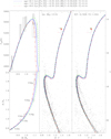 |
Fig. 6. Measurements of V56 and the eclipsing binaries V18 and V20 (left panels) and cluster CMDs (middle and right panels) compared to Victoria model isochrones and ZAHB loci as described in Brogaard et al. (2012). Uncertainties shown in the left panels are 1σ and 3σ for mass and radius of V18 and V20, but only 1σ for V56, and 1σ for all Teff values. GS_98 denotes the solar abundance pattern of Grevesse & Sauval (1998). The thick part of the ZAHB corresponds to masses with an RGB mass-loss from zero to twice the mean mass loss found from asteroseismology by Miglio et al. (2012). |
As seen in Fig. 6, an age close to 8.3 Gyr best reproduces the mass-radius relation as determined by V18, V20 and V56 together with the cluster CMD. In the past, age estimates of NGC 6791 varied quite a lot from one investigation to another, but with the mass-radius and mass-Teff relations constrained as they are now, the wiggle-room on the age has decreased significantly. This has implications for other works on, for example, the age of the cluster and on attempts to empirically calibrate asteroseismic scaling relations. Yet, surprisingly, there are still age estimates in recent literature that deviate quite a lot as detailed below.
4.1. Age in cluster catalogues
Kharchenko et al. (2013) determined log(age) = 9.645 for NGC 6791 corresponding to an age of only 4.42 Gyr. We inspected the details and found two issues that explain this as a systematic error caused by the facts that they assume solar metallicity and, most importantly, the photometry that they use does not reach the cluster turn-off and main sequence. This also explains why the distance that they determine along with the age, d = 4926 pc, was not problematic in their analysis: They were not limited by having to match the turn-off and main-sequence at all.
Cantat-Gaudin et al. (2020) used a set of open clusters with well-determined parameters in the literature to train an artificial neural network to estimate parameters (ages, extinctions, and distances) from Gaia photometry and parallax. For NGC 6791 they determined log(age) = 9.80, which translates to 6.31 Gyr. While being closer to our estimate than that of Kharchenko et al. (2013), it is still too young to seem trustworthy. The relatively low parallax value (=large distance) and especially the very large extinction value AV = 0.7 that they determined along with the young age enables a reasonable isochrone match to most of the CMD with their parameters, but the mass-radius relation would then be completely off for the binaries, the reddening much larger than any previous determination, and the observed red clump stars would be significantly brighter than the model. As mentioned by Cantat-Gaudin et al. (2020), their procedure does not account for variations in metallicity. We therefore suspect that their large extinction, which in turn causes their young age, is an artefact of the neural network trying to account for the high super-solar metallicity of NGC 6791 by increasing reddening and thus extinction.
4.2. Age and asteroseimic scaling relations
Kallinger et al. (2018) derived an age of 10.1 ± 0.9 Gyr and true distance modulus of (m − M)0 = 13.11 ± 0.03 for NGC 6791 based on asteroseismology of red giants along with empirical corrections to asteroseismic scaling relations. Their empirical corrections to the scaling relations were derived by forcing agreement between literature dynamical parameters (Gaulme et al. 2016; Brogaard et al. 2018b; Themeßl et al. 2018) and their own asteroseismic measurements for a sample of selected eclipsing binaries with an oscillating giant component. This requires that the dynamical parameters of eclipsing binary stars are reliable. However, their Fig. 11 shows that the age they derive for NGC 6791 is not consistent with the properties of the primary stars of the eclipsing members V18, V80 and V20. The disagreement is rather large; the x-axis is logarithmic and the mass of the V20 primary component is erroneously shown at a lower value rather than the true measurement of Brogaard et al. (2011) of 1.0868 ± 0.0039 M⊙. With the addition of the V56 primary properties from the present work, the discrepancy is now even more obvious. Their derived distance modulus for NGC 6791 also works against them: They assumed E(B − V) = 0.15 (T. Kallinger, priv. comm.) which yields (m − M)V = 13.575 adopting a standard AV = 3.1 × E(B − V). Comparing that to Fig. 6, this requires a slightly younger age than 8.3 Gyr, and is not consistent with their much older age close to 10 Gyr. Since there is no reason to put more reliance on the dynamical parameters of the binary stars used to derive the empirical corrections to the scaling relations than those of the binary stars in the cluster or even the cluster CMD, one must question the accuracy of both the age of NGC 6791 and scaling relation corrections derived by Kallinger et al. (2018). The cause of the problem is likely that the calibration sample used by Kallinger et al. (2018) is too small, which they also caution.
Brogaard et al. (2012) gave an estimate of the mass of the RGB stars at the V-band luminosity of the red clump in NGC 6791, MRGB, NGC 6791 = 1.15 ± 0.02 M⊙ and made a first comparison to early asteroseismic measures, showing that the asteroseismic scaling relations, which at that time were used without corrections, overpredicted the mass of RGB stars in NGC 6791 (Basu et al. 2011; Miglio et al. 2012). Those measurements, supported also by our new measurements of V56, now show that the empirical corrections suggested by Kallinger et al. (2018) make the scaling relations underpredict mass, since they suggest that the cluster RGB mass below the RC, 1.10 M⊙ as measured by Kallinger et al. (2018), is lower than the early SGB mass, 1.103 M⊙ as represented by V56p, at odds with stellar evolution theory. Theoretically predicted corrections to the asteroseismic scaling relations such as those of Rodrigues et al. (2017) are smaller than suggested empirically by Kallinger et al. (2018) and could lead to self-consistent results for the giant stars of NGC 6791, but their accuracy is still uncertain. Future attempts to further test and/or calibrate asteroseismology using NGC 6791 (Sharma et al. 2016; Pinsonneault et al. 2018) and additional open clusters and eclipsing binaries are therefore still needed.
5. Conclusions
We identified V56 as a non-eclipsing spectroscopic binary member of the open cluster NGC 6791 with two visible spectral components. Multi-epoch spectra were exploited in combination with prior knowledge and observations of NGC 6791 and its known eclipsing members to obtain masses, radii, Teff values and [Fe/H] for V56. These properties were then compared to isochrones, in combination with those of the eclipsing members V18 and V20 and the cluster CMD. This comparison support and strengthen the conclusions of Brogaard et al. (2012) with respect to a cluster age of 8.3 ± 0.3 Gyr and a mass of the RGB stars of MRGB, NGC 6791 = 1.15 ± 0.02 M⊙. These numbers therefore continue to serve as verification points for other age dating methods, such as various inferences from cluster CMDs and mass measures, for example in asteroseismology. We encourage the search for, and identification and exploitation of similar systems to V56 in other open clusters with known eclipsing binaries.
The disentangled spectra are available in tabular form as Tables A.1 and A.2 at the CDS.
Acknowledgments
We thank D. A. VandenBerg for assistance in the early stages of the project and for providing the stellar models used in Fig. 6. We thank the anonymous referee for useful comments. Based on observations collected at the European Southern Observatory under ESO programme 091.D-0125(A). We gratefully acknowledge the grant from the European Social Fund via the Lithuanian Science Council (LMTLT) grant No. 09.3.3-LMT-K-712-01-0103. Funding for the Stellar Astrophysics Centre is provided by The Danish National Research Foundation (Grant agreement no.: DNRF106). This research has made use of the SIMBAD database, operated at CDS, Strasbourg, France This paper includes data collected by the Kepler mission and obtained from the MAST data archive at the Space Telescope Science Institute (STScI). Funding for the Kepler mission is provided by the NASA Science Mission Directorate. STScI is operated by the Association of Universities for Research in Astronomy, Inc., under NASA contract NAS 5–26555.
References
- Basu, S., Grundahl, F., Stello, D., et al. 2011, ApJ, 729, L10 [NASA ADS] [CrossRef] [Google Scholar]
- Brogaard, K., Bruntt, H., Grundahl, F., et al. 2011, A&A, 525, A2 [NASA ADS] [CrossRef] [EDP Sciences] [Google Scholar]
- Brogaard, K., VandenBerg, D. A., Bruntt, H., et al. 2012, A&A, 543, A106 [NASA ADS] [CrossRef] [EDP Sciences] [Google Scholar]
- Brogaard, K., VandenBerg, D. A., Bedin, L. R., et al. 2017, MNRAS, 468, 645 [NASA ADS] [CrossRef] [Google Scholar]
- Brogaard, K., Christiansen, S. M., Grundahl, F., et al. 2018a, MNRAS, 481, 5062 [NASA ADS] [CrossRef] [Google Scholar]
- Brogaard, K., Hansen, C. J., Miglio, A., et al. 2018b, MNRAS, 476, 3729 [Google Scholar]
- Brogaard, K., Pakstiene, E., Grundahl, F., et al. 2021, A&A, 645, A25 [EDP Sciences] [Google Scholar]
- Bruntt, H., Grundahl, F., Tingley, B., et al. 2003, A&A, 410, 323 [NASA ADS] [CrossRef] [EDP Sciences] [Google Scholar]
- Cantat-Gaudin, T., Anders, F., Castro-Ginard, A., et al. 2020, A&A, 640, A1 [NASA ADS] [CrossRef] [EDP Sciences] [Google Scholar]
- Casagrande, L., & VandenBerg, D. A. 2014, MNRAS, 444, 392 [NASA ADS] [CrossRef] [MathSciNet] [Google Scholar]
- Coelho, P., Barbuy, B., Meléndez, J., Schiavon, R. P., & Castilho, B. V. 2005, A&A, 443, 735 [NASA ADS] [CrossRef] [EDP Sciences] [Google Scholar]
- Etzel, P. B. 2004, SBOP: Spectroscopic Binary Orbit Program (San Diego State University) [Google Scholar]
- Gaia Collaboration, 2018, VizieR Online Data Catalog, I/345 [Google Scholar]
- Gaulme, P., McKeever, J., Jackiewicz, J., et al. 2016, ApJ, 832, 121 [NASA ADS] [CrossRef] [Google Scholar]
- González, J. F., & Levato, H. 2006, A&A, 448, 283 [NASA ADS] [CrossRef] [EDP Sciences] [Google Scholar]
- Gray, D. F. 2009, ApJ, 697, 1032 [Google Scholar]
- Gray, R. O., & Corbally, C. J. 1994, AJ, 107, 742 [Google Scholar]
- Grevesse, N., & Sauval, A. J. 1998, Space Sci. Rev., 85, 161 [Google Scholar]
- Grevesse, N., Asplund, M., & Sauval, A. J. 2007, Space Sci. Rev., 130, 105 [Google Scholar]
- Gustafsson, B., Edvardsson, B., Eriksson, K., et al. 2008, A&A, 486, 951 [NASA ADS] [CrossRef] [EDP Sciences] [Google Scholar]
- Kallinger, T., Beck, P. G., Stello, D., & Garcia, R. A. 2018, A&A, 616, A104 [NASA ADS] [CrossRef] [EDP Sciences] [Google Scholar]
- Kaluzny, J., Pych, W., Rucinski, S. M., & Thompson, I. B. 2006, Acta Astron., 56, 237 [Google Scholar]
- Kaluzny, J., Thompson, I. B., Dotter, A., et al. 2014, Acta Astron., 64, 11 [Google Scholar]
- Kaluzny, J., Thompson, I. B., Dotter, A., et al. 2015, AJ, 150, 155 [NASA ADS] [CrossRef] [Google Scholar]
- Kharchenko, N. V., Piskunov, A. E., Schilbach, E., Röser, S., & Scholz, R. D. 2013, A&A, 558, A53 [NASA ADS] [CrossRef] [EDP Sciences] [Google Scholar]
- Knudstrup, E., Grundahl, F., Brogaard, K., et al. 2020, MNRAS, 499, 1312 [Google Scholar]
- Kuehn, C. A., Drury, J. A., Bellamy, B. R., et al. 2015, Eur. Phys. J. Web Conf., 101, 06040 [Google Scholar]
- Lightkurve Collaboration (Cardoso, J. V. d. M., et al.) 2018, Lightkurve: Kepler and TESS time series analysis in Python (Astrophysics Source Code Library) [Google Scholar]
- Meibom, S., & Mathieu, R. D. 2005, ApJ, 620, 970 [NASA ADS] [CrossRef] [Google Scholar]
- Meibom, S., Grundahl, F., Clausen, J. V., et al. 2009, AJ, 137, 5086 [NASA ADS] [CrossRef] [Google Scholar]
- Miglio, A., Brogaard, K., Stello, D., et al. 2012, MNRAS, 419, 2077 [Google Scholar]
- Mochejska, B. J., Stanek, K. Z., Sasselov, D. D., & Szentgyorgyi, A. H. 2002, AJ, 123, 3460 [NASA ADS] [CrossRef] [Google Scholar]
- Pasquini, L., Avila, G., Allaert, E., et al. 2000, SPIE Conf. Ser., 4008, 129 [Google Scholar]
- Pinsonneault, M. H., Elsworth, Y. P., Tayar, J., et al. 2018, ApJS, 239, 32 [Google Scholar]
- Platais, I., Cudworth, K. M., Platais-Kozhurina, V., et al. 2011, Am. Astron. Soc. Meeting Abstr., 218, 133.02 [Google Scholar]
- Rodrigues, T. S., Bossini, D., Miglio, A., et al. 2017, MNRAS, 467, 1433 [NASA ADS] [Google Scholar]
- Rucinski, S. M. 2002, AJ, 124, 1746 [Google Scholar]
- Sandquist, E. L., Jessen-Hansen, J., Shetrone, M. D., et al. 2016, ApJ, 831, 11 [NASA ADS] [CrossRef] [Google Scholar]
- Sharma, S., Stello, D., Bland-Hawthorn, J., Huber, D., & Bedding, T. R. 2016, ApJ, 822, 15 [Google Scholar]
- Slumstrup, D., Grundahl, F., Silva Aguirre, V., & Brogaard, K. 2019, A&A, 622, A111 [NASA ADS] [CrossRef] [EDP Sciences] [Google Scholar]
- Themeßl, N., Hekker, S., Southworth, J., et al. 2018, MNRAS, 478, 4669 [Google Scholar]
- Thompson, I. B., Kaluzny, J., Rucinski, S. M., et al. 2010, AJ, 139, 329 [NASA ADS] [CrossRef] [Google Scholar]
- Thompson, I. B., Udalski, A., Dotter, A., et al. 2020, MNRAS, 492, 4254 [Google Scholar]
- Tofflemire, B. M., Gosnell, N. M., Mathieu, R. D., & Platais, I. 2014, AJ, 148, 61 [NASA ADS] [CrossRef] [Google Scholar]
- Torres, G. 2010, AJ, 140, 1158 [NASA ADS] [CrossRef] [Google Scholar]
- Torres, G., Vanderburg, A., Curtis, J. L., et al. 2020, ApJ, 896, 162 [CrossRef] [Google Scholar]
- Zahn, J. P. 1977, A&A, 500, 121 [NASA ADS] [Google Scholar]
All Tables
All Figures
|
Fig. 1. Upper panel: SB2 orbit solution for V56. Red triangles are the RV measurements of the primary component and blue circles are the RV measurements of the secondary. Lower panel: O–C diagram of the RV measurements relative to the model in the top panel. |
| In the text | |
|
Fig. 2. V56 in the CMD of NGC6791. Grey dots are the photometry of NGC 6791 from Brogaard et al. (2012). The blue square represents the total light of V56. The blue line segments correspond to a range of pairs of V56 component magnitudes that combine to the total light magnitude while having one component on the cluster main sequence. The solid red lines give the V56 component V-band magnitudes as calculated from the total light magnitude and the spectroscopic light ratio. Dashed red lines are the corresponding 1σ uncertainties. Blue crosses are the best estimate V56 component magnitudes from the combined constraints of the cluster sequence and the spectroscopic light ratio. Green circles are the V18 component magnitudes. |
| In the text | |
|
Fig. 3. Photometric periods of individual Kepler quarters determined by-eye. Weighted average is 11.93 ± 0.02 days. |
| In the text | |
|
Fig. 4. Kepler light curves of V56 for selected quarters folded with the best estimate of the photometric period. |
| In the text | |
|
Fig. 5. Disentangled and renormalised spectra of the V56 components, primary on top, secondary below. The flux level of the secondary spectrum has been shifted from by −0.8 from 1 for clarity. The observed spectra are shown in black, the model spectra from Sect. 3.8 are overplotted in red. |
| In the text | |
|
Fig. 6. Measurements of V56 and the eclipsing binaries V18 and V20 (left panels) and cluster CMDs (middle and right panels) compared to Victoria model isochrones and ZAHB loci as described in Brogaard et al. (2012). Uncertainties shown in the left panels are 1σ and 3σ for mass and radius of V18 and V20, but only 1σ for V56, and 1σ for all Teff values. GS_98 denotes the solar abundance pattern of Grevesse & Sauval (1998). The thick part of the ZAHB corresponds to masses with an RGB mass-loss from zero to twice the mean mass loss found from asteroseismology by Miglio et al. (2012). |
| In the text | |
Current usage metrics show cumulative count of Article Views (full-text article views including HTML views, PDF and ePub downloads, according to the available data) and Abstracts Views on Vision4Press platform.
Data correspond to usage on the plateform after 2015. The current usage metrics is available 48-96 hours after online publication and is updated daily on week days.
Initial download of the metrics may take a while.