| Issue |
A&A
Volume 649, May 2021
|
|
|---|---|---|
| Article Number | A176 | |
| Number of page(s) | 10 | |
| Section | Stellar atmospheres | |
| DOI | https://doi.org/10.1051/0004-6361/202140620 | |
| Published online | 01 June 2021 | |
Wind suppression by X-rays in Cygnus X-3
1
Department of Physics, University of Helsinki,
PO Box 84,
00014,
Finland
e-mail: This email address is being protected from spambots. You need JavaScript enabled to view it.
2
Laboratory for High-Energy Astrophysics, NASA/GSFC, Greenbelt,
Maryland,
USA
3
Finnish Centre for Astronomy with ESO (FINCA), University of Turku,
Väisäläntie 20,
21500
Piikkiö,
Finland
4
Aalto University Metsähovi Radio Observatory,
PO Box 13000,
00076
Aalto,
Finland
5
Sky & Telescope,
One Alewife Center,
Cambridge,
MA
02140,
USA
Received:
20
February
2021
Accepted:
25
March
2021
Abstract
Context. The radiatively driven wind of the primary star in wind-fed X-ray binaries can be suppressed by the X-ray irradiation of the compact secondary star. This causes feedback between the wind and the X-ray luminosity of the compact star.
Aims. We aim to estimate how the wind velocity on the face-on side of the donor star depends on the spectral state of the high-mass X-ray binary Cygnus X-3.
Methods. We modeled the supersonic part of the wind by computing the line force (force multiplier) with the Castor, Abbott & Klein formalism and XSTAR physics and by solving the mass conservation and momentum balance equations. We computed the line force locally in the wind considering the radiation fields from both the donor and the compact star in each spectral state. We solved the wind equations at different orbital angles from the line joining the stars and took the effect of wind clumping into account. Wind-induced accretion luminosities were estimated using the Bondi-Hoyle-Lyttleton formalism and computed wind velocities at the compact star. We compared them to those obtained from observations.
Results. We found that the ionization potentials of the ions contributing the most to the line force fall in the extreme-UV region (100–230 Å). If the flux in this region is high, the line force is weak, and consequently, the wind velocity is low. We found a correlation between the luminosities estimated from the observations for each spectral state of Cyg X-3 and the computed accretion luminosities assuming moderate wind clumping and a low mass of the compact star. For high wind clumping, this correlation disappears. We compared the XSTAR method used here with the comoving frame method and found that they agree reasonably well with each other.
Conclusions. We show that soft X-rays in the extreme-UV region from the compact star penetrate the wind from the donor star and diminish the line force and consequently the wind velocity on the face-on side. This increases the computed accretion luminosities qualitatively in a similar manner as observed in the spectral evolution of Cyg X-3 for a moderate clumping volume filling factor and a compact star mass of a few (2–3) solar masses.
Key words: binaries: general / stars: winds, outflows / stars: black holes / accretion, accretion disks / radiative transfer
© ESO 2021
1 Introduction
Cygnus X-3 (4U 2030+40) was one of the first X-ray binaries discovered (Giacconi et al. 1967) and is also one of the brightest. It is listed in the Catalogue of High-Mass X-ray Binaries in the Galaxy (Liu et al. 2006), where most entries consist of an OB star whose wind feeds a companion neutron star or a black hole, releasing X-rays in the process. The donor star of Cyg X-3 (optical counterpart V1521 Cyg) is a massive Wolf-Rayet (WR) star of either of type WN 5-7 (Van Keerkwijk et al. 1992, 1996) or a weak-lined WN 4-6 (Koljonen & Maccarone 2017). The relatively small size of this helium star allows for a tight orbit with a period of 4.8 h that is more typical of low-mass X-ray binaries. In this paper we study the effect of soft X-rays (EUV radiation) on various wind models of the WR star and estimate the corresponding accretion rates and luminosities during different spectral states of Cyg X-3.
Sander et al. (2017) presented three different approaches for handling the radiative transfer of line-driven winds of hot stars. The first is an analytical description based on the concept of the CAK theory (Castor et al. 1975). This method has also opened up the whole area of time-dependent and multidimensional calculations (see, e.g., Sundqvist et al. 2010). The CAK theory assumes that line broadening is dominated by the bulk motion of the wind. In a rapidly expanding wind, line saturation is avoided, which leads to a strong line force. The second approach is to calculate the radiative force with the help of Monte Carlo (MC) methods. Computationally, the MC method is much more time-consuming than the CAK method. The third approach is to calculate the radiative transfer in the comoving frame (CMF; see Krticka & Kubat 2017; Krticka et al. 2018; Sander et al. 2018). This method has also been applied to WR stars (Sander et al. 2017; Hamann et al. 2006; Hainich et al. 2014).
X-rays (mainly soft X-rays in the extreme-UV, EUV, region) from the compact star affect the wind through photoionization. An increase in highly ionized ions may decrease the line-driven mechanism and reduce the wind velocity. As noted by Karino (2014), pioneering work on these ionized wind dynamics was done by Stevens & Kallman (1990), who used the XSTAR code (Kallman 2018) to approximate the wind with a photoionized plasma; the line force was computed with the CAK method. In the present paper, we revisit and further develop this method and apply it to Cyg X-3. We adopt the first approach (CAK) classified by Sander et al. (2018). The results we present agree with those of Krticka et al. (2018) for HMXRBs: X-rays reduce the wind velocity, and wind clumping weakens the effect of X-rays. Szostek & Zdziarski (2008) found that the wind of Cyg X-3 has to be clumpy in order to explain the observed X-ray absorption. We therefore include clumping with different filling factors here.
Our goal is to study the penetration of X-rays from the compact star of Cyg X-3 of the wind, and to determine how it affects the wind properties, in particular, the wind velocity between the two stars. Based on this, we estimate the accretion luminosities of the five main spectral states of Cyg X-3 as classified by Hjalmarsdotter et al. (2009). Macgregor & Vitello (1982) applied a somewhat similar approach to X-ray binary systems with wind accretion and found that X-ray irradiation diminishes the wind velocity. A relevant recent paper (and references therein) is on Cyg X-1 by Meyer-Hofmeister et al. (2020). They found that the outflow from the OB-star facing the X-ray source is noticeably slower than from the opposite hemisphere in the X-ray shadow. Furthermore, they give evidence for two stable states: the soft high-luminosity state, and the hard low-luminosity state.
2 Cyg X-3 system parameters
Using Chandra High Energy Transmission Grating data (HETG, ObsID 7268 and 6601), Vilhu et al. (2009) derived radial velocity curves of the FeXXVI emission line at 1.78 Å (H-like), which is thought to originate in the vicinity of the compact star. These data comprise ten phase bins and give a radial velocity i amplitude of 454 ± 109 km s−1. When this is coupled with that of the infrared HeI absorption line (thought to originate in the WR component) of 109 ± 13 km s−1 (Hanson et al. 2000), it yields a mass ratio MC /MWR = 0.24 ± 0.06. Zdziarski et al. (2013) arrived at a similar number using the same data, but selecting a slightly different subset of the data. Based on the statistics of the masses and mass-loss rates of WR stars, Zdziarski et al. (2013) fixed the WR companion mass at about 10 M⊙. This implies a mass of 2.4 M⊙ for the compact star. We use these values in the present paper. Zdziarski et al. (2013) estimated the mass-loss rate to be between (4.8–8.2) × 10−6 M⊙ yr−1. We adopted the mean value 6.5 × 10⁻⁶ M⊙ yr−1, which is close to that derived from the orbital period increase Ṁ = Mtot(Ṗ/2P) (Ergma & Yungelson 1998).
Based on Gemini/GNIRS infrared spectroscopy, Koljonen & Maccarone (2017) suggested that the WR component is of spectral class WN 4-6 and that its bolometric luminosity lies between (5.5–11.5) × 1038 erg s−1. We adopted 8.0 × 1038 erg s−1 as a compromise value. For the photospheric blackbody temperature we adopted 1.25 × 10⁵ K. The WRcomponent radius at the wind base and the binary separation are 0.95 and 3.31 solar radii, respectively.The temperature and radius of the adopted model are close to those of the Potsdam WNE model 15-211.
As the WR component is a hydrogen-deficient WN star, we adopted hydrogen, helium, and heavy element mass fractions of X = 0.085, Y = 0.90, and Z = 0.015, respectively (Nugis & Lamers 2000). We used solar abundances for individual heavy elements (Asplund et al. 2009). The effect on the force multiplier of using equilibrium CNO abundances is negligible. We assigned a distance of 7.4 kpc based on Mccollough et al. (2016). The system parameters are collected in Table 1.
3 EUV photon fluxes in the spectral states of Cyg X-3
The hybrid EQPAIR model originally developed by Coppi (1992) is suitable for modeling the broadband X-ray spectrum of Cyg X-3 (Vilhu et al. 2003; Hjalmarsdotter et al. 2009). At soft X-rays below 0.1 keV, which are not observable due to high circumstellar and interstellar absorption, the model is dominated by disk blackbody and Compton scattering from thermal electrons.
Using a large dataset of RXTE X-ray observations, Hjalmarsdotter et al. (2009, see their Fig. 7, reproduced here as Fig. 1) classified the model into five main states (hard, soft nonthermal, intermediate, ultrasoft, and very high). Table A.1 gives the model fluxes at 100 eV (unabsorbed at Earth). From these fluxes and spectral shapes of Fig. 1, the unabsorbed number of photons between 100–230 Å (54–124 eV, where 54 eV is the HeII ionization edge) was estimated. These EUV photons are important because they decrease the size of the line force. A similar effect is in the increase of ionization due to X-rays (see Appendix B). The EUV flux of the hard state is uncertain due to the absorption, as noted by Zdziarski et al. (2016).
The ionization potentials of NiV and FeV (four electrons stripped off), the lines of which contribute to the line force, fall into the 100–230 Å region. As an example, photons between 70 and 90 eV can ionize FeV (Fe4+; see, e.g., El Hassan 2009). If the radiator has significant flux in this region, these ions are photoionized and the line force decreases. Other smaller contributors to the line force are the lines of CIV, NV, and CrV ions, for instance, whose ionization potentials also fall in this region. For the effect of EUV photons on the line force as well as for a computation of the line force, see Appendix B.
Parameters of the Cyg X-3 binary components and stellar wind used in this paper.
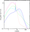 |
Fig. 1 Unabsorbed model spectra of the five main accretion states of Cyg X-3 reproduced from Hjalmarsdotter et al. (2009). The models corresponding to the hard state (solid blue line), the intermediate state (long-dashed cyan line), the very high state (short-dashed magenta line), the soft nonthermal state (dot-dashed green line), and the ultrasoft state (dotted red line) are shown (unabsorbed at Earth). |
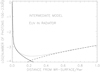 |
Fig. 2 Number of photons between 100 and 230 Å (in units of that from a 125 000 K blackbody) as a function of the distance from the WR star surface (the intermediate model of Table A.1 (fvol = 0.3, Φ = 0) along the line joining the stars). The compact star is located at 2.4 RWR. The solid line shows the contribution from the WR star and the dashed line that from the compact star (X-ray source). The dotted line shows the coadded contribution. |
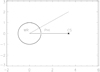 |
Fig. 3 Geometry of the system in the orbital plane in units of the WR star radius. The compact star (CS) is located at distance 3.4 from the center of the WR star. The orbital angle Φ (PHI) is marked in the direction of the motion of the compact star. |
4 Computation of wind velocities
Wind models were computed for each of the five spectral states taking into account the effect of X-rays from the compact star. The wind equations were solved along the line joining the centers of the two stars (Φ = 0) and for different orbital angles Φ (see Fig. 3). The geometry is the same as in Krticka et al. (2012, see their Fig. 1). We also repeated their Vela X-1 computations with the present XSTAR method, and these are outlined in Appendix C, along with comparisons with the CMF method for O stars from Krticka & Kubat (2017).
Soft X-rays from the compact star penetrate the wind from the donor star and change the radiation field and the number of photons in the critical EUV range 100–230 Å. In numerical computations, fluxes from inside (WR star) and outside (compact star) were computed at each wind layer. The WR flux was set to 125 000 Kblack body at the surface and modified in the wind by absorption (stored in a precomputed grid) depending on wavelength, ionization, density and composition. Figure 2 shows the relative number of photons between 100 and 230 Å as a function of the distance from the WR surface (intermediate state at Φ = 0). The local force multiplier (line force) was then computed using the coadded 100–230 Å fluxes from the WR and compact stars, respectively. Higher EUV flux corresponds to a weaker line force.
We considered only the supersonic part of the wind flow (above δ(r∕RWR) = 0.01 from the WR surface). As shown in Fig. 2, EUV photons from the compact star do not penetrate the sonic point, only the outer part of the supersonic wind is affected. At this boundary, the wind velocity was set to 25 km s−1, slightly above the sonic point for a 105 K He gas, which isabout 20 km s−1. A better estimate of the sonic point properties can be found in Grassitelli et al. (2018). For a He-star model of 10 M⊙ and mass-loss rate of 8 × 10⁻⁶ M⊙ yr−1 (close to the Cyg X-3 value in Table 1), they find a velocity of 19.62 km s−1 at the sonic point (see their Table 1). Below this boundary, the wind particle column was assumed to be 1023 cm−2 (the whole wind column is 20 times larger). The wind velocity scales with this column loosely as (column)0.1. For the model without X-rays, the assumedcolumn gives Vinf ≈ 2200 km s−1 (NOX in Fig. 4).
The wind was divided into 1000 shells with δ(r∕RWR) = 0.01. The mass-loss rate was kept constant, and we assumed that it is determined in the subsonic part of the wind that X-rays from the compactstar do not penetrate. The gravitational pull of the compact star was not included. Clumping was included assuming that all the wind mass is in the clumps and that the space between clumps is empty. In this case, the particle number density N in the ionization parameter ξ (Eq. (B.4)) is replaced by N/fvol, where fvol is the volume-filling factor. Clumping makes ξ smaller, increasing the line force and consequently the wind velocity (see Fig. B.4).
The two equations which determine the flow are mass conservation
 (1)
(1)
and momentum balance (neglecting gas pressure)
![Mathematical equation: \begin{equation*} v\textrm{d}v/\textrm{d}r = GM/r^{2} [\Gamma_{\textrm{e}}(1 + g_{\textrm{line}}) - 1] \, {\rm} ,\end{equation*}](/articles/aa/full_html/2021/05/aa40620-21/aa40620-21-eq3.png) (2)
(2)
where the line force is
 (3)
(3)
and
 (4)
(4)
Using the values in Table 1 for the WR star yields Γe = 0.34. The value of the finite disk correction factor Fd(r) is about 0.7 at the WR surface and increases to 1 at x = r∕RWR = 1.5. It remains constant thereafter (Sundqvist et al. 2014). The force multiplier FM depends on the ionization parameter ξ, the absorption parameter t (Eq. (B.1)), and the spectral shape of the radiator, particularly in the EUV region around 100–230 Å. In practice, FM was interpolated from an extensive precomputed grid at each wind layer using local values of these parameters (see Appendix B).
The wind equations were integrated numerically from x = r∕RWR = 1.01 up to 10.0, resulting in velocity stratification v(r) (see Fig. 4). Without X-rays the resulting velocity stratification can be compared and fitted with a standard β-velocity model to give the best model (see Appendix C.1). However, with X-ray irradiation, no such standard model exists, and we used our own formula in which the β-velocity model is multiplied by a suppression factor SF,
 (5)
(5)
![Mathematical equation: \begin{eqnarray*} \textrm{SF} &=& \begin{cases} 1 - \textrm{slope} \,{\times}\, (x - xkink), & \text{if}\ x \geq xkink \\ 1, & \text{if}\ x < xkink \end{cases} \\[10pt] B &=& 1.01\,{\times}\,[1 - (v_{\textrm{in}}/v_{\textrm{inf}})^{1/\beta}] \\[10pt] x &=& r/R_{\textrm{star}}, \end{eqnarray*}](/articles/aa/full_html/2021/05/aa40620-21/aa40620-21-eq7.png)
where the slope and xkink are fitting parameters. In the inner boundary, vin = 25 km s−1.
The fits were improved by integrating the wind equations several times (without fitting), computing the EUV contamination from the previous model, until the average difference between two subsequent models was smaller than 1%. This typically required 10–20 runs. The results do not differ much from the case where the X-rays were simply switched on in the NOX-model (no X-rays) and the model integrated without fitting. The computation for Φ = 0 (along the line joining the centers of the two stars) is straightforward. For larger angles, we numerically integrated across the wind to obtain dilution factors and absorption. Following Krticka et al. (2012), we assumed that the wind in the direction of the orbital angle Φ can be modeled by a spherically symmetric wind.
The resulting wind velocity in the NOX state is compatible with velocities of WN stars derived from line widths of He lines (Hamann et al. 1995). Computations with different orbital angles are relevant because the time in which the wind element crosses the distance between the components (crossing time) is about 0.35–0.45 h for our models, corresponding to orbital angles between 25 and 35 degrees (see Table A.1). The true wind velocity at the compact star is likely a smear of computed velocities inside Φ = 0–35 degrees.
Figure 4 (left panel) shows the velocity stratifications for three spectral states at Φ = 0 and moderate clumping (fvol = 0.3). In addition, orbital angles of 30 and 90 degrees are included for the intermediate state. The right panel of Fig. 4 shows velocity stratifications for the very high state with several clumping filling factors. At large distances from the WR star, the velocities approach constant values. This plot can be compared with a similar one from Krticka et al. (2018, their Fig. 4). For small clumping filling factors (fvol < 0.1), the wind velocity and accretion luminosity become rather insensitive to the EUV flux (see Table A.1 and Fig. 5) because clumping causes the ionization ξ parameter to decrease and consequently the EUV dependence to weaken (see Fig. B.4).
The wind velocity around the compact star during the very high state is consistent with the P Cygni absorption of the SiXIV line at −900 ± 750 km s−1, which is observed most clearly at about orbital phase 0.5 (compact star in front, WR star behind; Vilhu et al. 2009). For more details on P Cygni lines and photoionization in Cyg X-3, see also Kallman et al. (2019). In the next section we estimate the accretion rates and luminosities from the computed velocities at the compact star and compare them with those from the EQPAIR models. The wind velocities were computed without the gravitational pull of the compact star to show the effect of X-rays and to apply the Bondi-Hoyle-Lyttleton model in the next section.
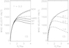 |
Fig. 4 Left panel: computed wind velocities as a function of the radial distance from the center of the WR star (in units of stellar radius) for the orbital angle Φ = 0 deg (solid lines, see Fig. 3). The clumping volume filling factor f = fvol = 0.3. VH = very high state, INT = intermediate state, HARD = hard state, and NOX = the wind without X-rays from the compact star (whose distance is marked as CS in the plot). Dashed lines are for the intermediate state for angles Φ = 30 deg (lower) and 90 deg (upper). Right panel: wind radial velocities for the very high state with three clumping volume filling factors f = fvol = 1.0, 0.3, and 0.1 (dashed lines). The solid line shows the wind without X-rays (NOX) and with f = 0.3. The gravitational pull of the compact star is not included. |
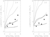 |
Fig. 5 Left panel: computed accretion luminosities (in units of 1038 erg s−1) for thefive spectral states of Cyg X-3 are shown for three clumping filling factors f = fvol = 1.0 (dotted lines), = 0.3 (dashed lines), and = 0.1 (solid lines). The orbital angle Φ = 0 deg for the upper curves and Φ = 30 deg for the lower ones. The filled squares show the EQPAIR model luminosities (Lbol of Table A.1) The compact star mass is 2.4 M⊙. In the abscissa 0 indicates NOX (no X-rays), 1 hard, 2 soft nonthermal, 3 intermediate, 4 ultrasoft, and 5 very high state. Right panel: same as in the left panel, but the compact star mass is 3.0 M⊙. |
5 Accretion luminosities during Cyg X-3 spectral states
Using wind velocities at the compact star and a simple analytic wind accretion model described by Frank et al. (1992), we estimate the accretion luminosity Lacc. This Bondi-Hoyle-Lyttleton model has been used widely for instance by Watanabe et al. (2006), Koljonen & Maccarone (2017), and Krticka et al. (2018). A review of the topics with original references can be found in Martinez et al. (2017). In the previous section, wind velocities were computed without the gravitational pull of of the compact star because in the Bondi-Hoyle-Lyttleton model, the wind velocity is taken at the distance of the compact star and without its gravitational pull. This is taken into account when deriving the formula itself, which should only be considered as a sort of scaling law. In the model, Lacc strongly depends on the relative velocity Vrel,
 (9)
(9)
where the orbital velocity of the compact star is Vorb = 675 km s−1 using the system parameters in Table 1. The accretion luminosity is
 (10)
(10)
where the accretion rate depends on the accretion radius as follows:
 (11)
(11)
 (12)
(12)
The mass-to-energy conversion factor η = 0.1 was used, which is approximately valid for neutron stars and black holes (see, e.g., Frank et al. 1992). Accretion luminosities were calculated for the five spectral states using the computed wind velocities at the compact star (see Fig. 4 and Table A.1) for three clumping filling factors fvol = 1.0 (no clumping), 0.3, and 0.1. These are shown in Fig. 5. The filled squares in Fig. 5 show the EQPAIR model luminosities (Lbol of Table A.1).
The left panel of Fig. 5 shows the luminosities computed for the compact star mass 2.4 M⊙, and the right panel shows the luminosities for a higher compact star mass 3.0 M⊙. Because the realistic wind velocity probably lies between orbital angles 0 and 30 degrees (30 deg is close to the crossing times in Table A.1), moderate clumping favors 2.4 M⊙ and higher clumping favors 3.0 M⊙. Lower masses require less clumping. At very high clumping, the correlation between different spectral states disappears.
Fitting the mean bolometric luminosity value of spectral states (Lbol = 2 × 1038 erg s−1) with similar means from our computations at orbital angle Φ = 15 degrees, we derived the relation between the clumping filling factor and compact star mass (fvol, MC): (0.70, 1.4), (0.28, 2.0), (0.16, 2.4), and (0.08, 3.0). Szostek & Zdziarski (2008) estimated values between 0.07 and 0.3 for the one-phase filling factor (used in the present work). This points to a compact star mass between (2–3) M⊙.
6 Discussion
We computed the force multiplier (line force) using the CAK method, and the wind was approximated by the photoionized plasma codeXSTAR (Stevens & Kallman 1990; Kallman 2018). XSTAR is designed to calculate the ionization and thermal balance in gases exposed to ionizing radiation. It contains a relatively complete collection of relevant atomic processes and corresponding atomic data. It does not by itself include processes associated with wind flows, such as shock heating, adiabatic cooling, or time-dependent effects. It also has a simple treatment of radiation transport that provides approximate results in situations involving truly isotropic radiation fields or line blanketing, for example.
Key simplifications employed by XSTAR are with regard to the radiative transfer solution. Escape of line radiation is treated using an escape probability formalism, and this affects the temperature through the net radiative cooling. Transfer of the ionizing continuum is treated using a single-stream integration of the equation of transfer, including opacities and emissivities calculated from the local level populations. Thus, there is no allowance for the inward propagation of diffusely emitted radiation.
This last approximation is likely to be most important for the results presented here because strong winds can have large optical depths in the ionizing continua of H and He II. It would be desirable to verify our current results for the force multiplier using a transfer solution that does not have this limitation. Limitations of the escape probability assumption for line escape have been pointed out by Hubeny et al. (2001), for example. However, for hot star winds, the strong velocity gradient reduces most line optical depths to approximately a few at most, and so the lines are effectively thin and the radiative cooling is not strongly affected. However, the simplifications made do not affect the EUV sensitivity of the force multiplier, which is the key issue here.
The assumed masses for the components may represent just one possible solution for Cyg X-3. A more massive possibility within errors is 3.0 + 10 M⊙, for example, yielding 50% higher computed accretion luminosities. A less massive alternative 2.0 + 10 M⊙ yields the opposite. A tolerable match with the EQPAIR models can be provided by moderate clumping (fvol = 0.1 – 0.3) and MC = 2.4 M⊙ or by fvol = 0.1 and MC = 3.0 (see Fig. 5). Smaller compact star masses require less clumping, which is an unknown parameter in this study. However, typical volume filling factors for WR-stars have been estimated to be 0.1–0.25 (e.g., Hamann & Koesterke 1998).
The region in which the photoionization of the main contributors to the line force takes place was assumed to be 100–230 Å. However, this region could be shallower, for instance, 100–177 Å, because the ionization potentials of the main contributors NiV and FeV are at 164 Å. In this case, the computed accretion luminosities would increase (by a factor of 1.5). One possible caveat is that the estimated EUV fluxes from the EQPAIR models do not necessarily reflect reality. In a sense, the EUV flux is always model dependent because we cannot obtain any observations in these wavelengths.
Accretion disks are frequently assumed in the context of wind accretion. Accretion disk formation in radiatively driven wind accretion has recently been studied by Karino (2019). A good illustration of the Cyg X-3 disk can be found in Hjalmarsdotter et al. (2009). The origin of transitions between the different states probably lies in some form of disk instability. In the hard state, the radius of the inner accretion flow is large (and the EUV flux low). In the soft states, the inner disk boundary shrinks, and consequently, the EUV flux increases, the wind velocity decreases, and the accretion luminosity Lacc increases (see Fig. 7 in Hjalmarsdotter et al. 2009 and discussion therein).
The disk and wind may interact. This means that the changing EUV flux from the compact star might account for the different luminosity and spectral states of Cyg X-3. When the EUV flux is high, the X-ray accretion luminosity is also high, and vice versa. Our computations together with the EQPAIR model luminosities favor this picture if both the compact star mass and clumping are suitable (see Fig. 5). We might speculate that during an eventual extremely high state (flare) the computed wind at the compact star may stop, the X-ray production ends, and the wind returns to the NOX state. During this state, the accretion luminosity does not differ much from the hard-state luminosity (see Fig. 5). The hard state may thus be the most natural and long-lasting state of Cyg X-3.
Antokhin & Cherepashchuk (2019) extended the list of times of X-ray minima and fit the O− C diagram by a sum of quadratic and sinusoidal (with period 15.79 yr) functions. They suggested the existence of either apsidal motion or a third body. The mass loss, causing the period increase, is behind the overall shape of the O− C diagram. For the quadratic plus sinusoidal ephemerides, Antokhin and Cherepashchuk find Ṗ = 5.629 × 10⁻¹⁰, corresponding to a relative period change of Ṗ /P = 1.029 × 10⁻⁶ yr−1. Ṗ is related to the coefficient c of the quadratic term by c = PṖ/2. We estimate the change of Ṗ /P in our models below.
For a nonconservative mass transfer by fast isotropic wind (Jeans mode, see Ziolkowski & Zdziarski 2018, their Eq. (15) with α = 1):
![Mathematical equation: \begin{equation*} \frac{ \dot P}{P}= \frac{\dot M_{\textrm{wind}}}{M_{\textrm{WR}}}\left[3 - 3\beta \frac{M_{\textrm{WR}}}{M_{\textrm{C}}}-(1-\beta)\frac{M_{\textrm{WR}}}{M_{\textrm{tot}}}-3(1-\beta)\frac{M_{\textrm{C}}}{M_{\textrm{tot}}}\right] ,\end{equation*}](/articles/aa/full_html/2021/05/aa40620-21/aa40620-21-eq12.png) (13)
(13)
where β is the fraction of the wind accreted by the compact star Ṁacc/Ṁwind.
For an acceptable model (10 M⊙ + 2.4 M⊙, fvol = 0.16, see Sect. 5), we have β = 0.002 and 0.005 for the hard state and the very high state, respectively. For the period change, these give Ṗ /P values 1.034 × 10⁻⁶ yr−1 (hard) and 1.012 × 10⁻⁶ yr−1 (very high), which differ by 2%. Hence, the effect of spectral states on the O− C diagram is very small through the quadratic term coefficient. Moreover, in the ASM∕RXTE data, Cyg X-3 spent 50% of the time in the low state (<10 cps) and 22% in the high state (>20 cps). Hence, the average of Ṗ /P is closer to the hard-state value as observed. Locally, like during and after the jigsaw pattern detected in the ASM∕RXTE data between MJD = 50 700–51 600 (when Cyg X-3 was mostly in the low hard state), this effect is unobservable. The jigsaw pattern is probably caused by the temporal irregular distribution of ASM data, as suggested by Antokhin and Cherepashchuk.
7 Conclusions
We constructed wind models in the supersonic part of the WR component of Cyg X-3 using force multipliers (line force) computed with CAK formalism and XSTAR physics (following the pioneering work of Stevens & Kallman 1990; for the XSTAR-code, see Kallman 2018). The line force strongly depends on the EUV flux of the radiator (100–230 Å), to which the X-rays from the compact star contribute. The main contributors are lines of NiV and FeV ions (to a lesser extent, e.g., CIV, NV, and CrV). Their (photo)ionization potentials fall between 100 and 230 Å (54–124 eV). In this region the radiation field controls these lines and consequently the size of the force multiplier. Higher EUV flux from the compact star means a weaker line force, which in turn leads to a lower wind velocity.
Because X-rays do not reach the subsonic part of the wind, we assumed that the mass-loss rate is unaffected by X-rays. We included clumping by assuming that all the wind mass is in the clumps. We modeled the wind at different orbital angles (see Fig. 3). Computations with different orbital angles are relevant because the time in which the wind element crosses the distance between the components (crossing time) is about 0.35–0.45 h in our models. This corresponds to orbital angles between 25 and 35 degrees (see Table A.1).
Radiation from the compact component increases the EUV flux and diminishes the wind velocity (Fig. 4). This enhances the accretion rate, and consequently, the accretion luminosity (Fig. 5). The computed Bondi-Hoyle-Lyttleton inosities Lacc correlate moderately well with the luminosities of the five main spectral states of Cyg X-3 defined by Hjalmarsdotter et al. (2009), provided that the clumping is moderate (fvol = 0.1–0.3) and the mass of the compact star is about(2–3) M⊙ (with the WR-star mass 10 M⊙, see Fig. 5). For higher clumping (fvol ≪ 0.1) the EUV sensitivity disappears because clumping decreases the ionization parameter ξ and the line force dependence on EUV flux (see Fig. B.4).
We compare our XSTAR method with the CMF method (comoving frame) in Appendix C. The results are qualitatively similar for both O stars (Krticka & Kubat 2017) and X-ray suppression in Vela X-1 (Krticka et al. 2012).
Acknowledgements
We thank Drs. Hjalmarsdotter and Krticka for permission to use their figures (Figs. 1 and C.3) and Drs Andrzei Zdziarski and Linnea Hjalmarsdotter for valuable comments. K.I.I.K was supported by the Academy of Finland projects 320045 and 320085.
Appendix A Computed wind velocities
In Table A.1 we list the EUV/EQPAIR fluxes and bolometric luminosities of Cyg X-3 spectral states (Hjalmarsdotter et al. 2009) and the computed wind velocities at the compact star (this study).
Luminosities and EUV-fluxes of the five basic states of Cyg X-3 from RXTE observations and EQPAIR models (Hjalmarsdotter et al. 2009, first two rows) and computed wind velocities at the compact star (this study, last rows).
Appendix B Methods for computing the line force (force multiplier). Effect of EUV photons.
The force multiplier (line force) FM was computed following the method described by CAK. An important difference is that CAK (and other compilations, e.g., Gayley et al. 1995) assume that the ionization and excitation in the wind is given by the Saha-Boltzmann distribution modified by an analytic dilution factor applied to all elements. We computed the ionization distribution in the wind by balancing the ionization and recombination due to the stellar radiation field. We also employed the Boltzmann distribution to determine the populations of excited levels. The radiation field was computed using a single-stream integration outward from the stellar photosphere. In this way, we calculated the line force appropriate to any spectral form of the photospheric spectrum and at any layer in the wind. This permitted us to integrate wind equations from the surface to infinity in a self-consistent manner because the upward force is known.
The ionization balance and outward transfer of photospheric radiation were calculated using the XSTAR photoionization code (Stevens & Kallman 1990; Kallman 2018). The ion fractions at each spatial position in the wind were used to calculate the force multiplier FM by summing the CAK line force expression over an ensemble of lines. The list of lines was taken from Kurucz2 and permitted us to use local wind parameters. The line list is more extensive than in the original CAK work. It is assumed that the wind is spherically symmetric around the donor star (the ionizing source).
XSTAR calculates the ionization balance for all the elements with atomic number Z ≤ 30 together with the radiative equilibrium temperature. It calculates full nonlocal thermal equilibrium (NLTE) level populations for all the ions of these elements. It includes a fairly complete treatment of the level structure of each ion, that is, more than ~50 levels per ion, and up to several hundred levels for some ions. Many relevant processes affecting level populations are included such as radiative decays, electron impact excitation and ionization, photoionization, and Auger decays. The electron kinetic temperature is calculated by imposing a balance between heating from fast photoelectrons and Compton scattering with radiative cooling.
For a fixed radiator, the force multiplier FM(t, ξ, N) is a three-dimensional function of the absorption parameter t, ionization parameter ξ (erg s−1 × cm), and particle number density N (cm−3),
 (B.1)
(B.1)
 (B.2)
(B.2)
Here Lly is the radiation luminosity below the hydrogen ionization limit 912 Å, σe is the electron scattering coefficient, ρ and N are the gas and particle number density, respectively, v is the outward wind velocity, r is the radial distance from the ionizing source, and vth is the gas thermal velocity (typically ~10 km s−1). The dependence on N is weak (Kallman et al. 2019). The force multiplier was computed assuming a point source radiator. When applied to stars, the dilution factor r−2 in ξ (Eq. (B20)) should be replaced by the finite disk factor (Mewe & Schrijver 1978),
![Mathematical equation: \begin{equation*} W(r) = 0.5[1 - \sqrt(1 - (R_{\textrm{star}}/r)^2)]R_{\textrm{star}}^{-2}. \end{equation*}](/articles/aa/full_html/2021/05/aa40620-21/aa40620-21-eq15.png) (B.3)
(B.3)
In our paper the radiator consists of two sources: the WR-star and the (point source) compact star. The ionization parameter was computed taking the (absorbed) contributions Llywr and Llyx from both sources into account,
 (B.4)
(B.4)
where rwr and rx are the distances from the WR center and compact star, respectively. Llywr and Llyx are component luminosities below the Lyman edge at a specific point in the wind, absorbed along the path from the WR-surface and the compact star (X-ray source), respectively (by exp(-absorption × column)). X-rays increase the ionization parameter ξ through the Lyman luminosities and diminish the line force. In the case of Cyg X-3, the EUV-photons from the compact star are more important. Their number effectively controls the line force.
The chemical abundances of the wind and the ionizing source spectrum can be specified as input data. The method is in principle the same as in the classical work of CAK. However, we explicitly included ξ and t and computed it locally in the wind. In the case of clumping, with volume-filling factor fvol and all mass in the clumps, the particle number density N in Eq. (B.2) should be replaced by N/fvol.
The force multiplier depends on t and on the cross section for line absorption,
 (B.5)
(B.5)
where ΔνD is the thermal Doppler width of the line, F is the total flux in the continuum, Fν is the monochromatic flux at the line energy, and
 (B.6)
(B.6)
 (B.7)
(B.7)
where NL and NU are the lower and upper level populations, gi are the statistical weights, and f is the oscillator strength. Our code (xstarfmult.f) uses the ion fractions calculated as described above to sum over lines to calculate FM (t, ξ). Ground-state level populations were taken directly from XSTAR; excited level populations were calculated assuming a Boltzmann (LTE) distribution. This is necessitated by the use of the Kurucz line list, which does not include collisional rates or other level-specificquantities that would allow a full NLTE calculation of populations. Most previous calculations of the CAK force multipliers have employed the LTE assumption for excited levels as well (e.g., CAK; Abbott 1982; Gayley et al. 1995).
FM grids were computed for the chemical composition of WNE stars for many ξ- and t-values and radiators around 125 000 K blackbody with different amounts of flux cut below 230 Å. Cut blackbodies give the same size force multipliers as realistic absorbed models (Vilhu & Kallman 2019, their Figs. 2 and 3). In the course of computations, at a fixed layer in the wind, the real absorbed radiator spectrum was compared with the grid spectra and FM interpolated together with local ξ and t values. The EUV contamination of the X-ray source was included. A black body radiator was assumed at the surface and modified in the wind by absorption (from a precomputed grid) depending on wavelength, ionization parameter, density and chemical composition.
The lines of NiV and FeV ions are the strongest contributors to the force multiplier (in addition to, e.g., CIV, NV, and CrV). The lines are mainly in the Lyman-continuum below 912 Å. When these ions ionize, the lines disappear, and consequently, the force multiplier becomes smaller. This ionizing takes place if the radiator has significant flux below 230 Å. Figures B.1 and B.2 show this effect for a 135 000 K blackbody (slightly differing from 125 000 K of Table 1) as a function of element atomic number and wavelength. Figure B.3 shows the mean ionization weighted by the contribution to the force multiplier (4 means that four electrons are stripped off). The soft X-ray suppression clearly vanishes when flux below 230 Å is absorbed, which increases the contribution of the iron group elements. This property of force multiplier also helps to explain the momentum problem of WR winds (Vilhu & Kallman 2019).
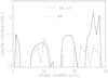 |
Fig. B.1 Contributions to the force multiplier (FM) as a function of the element atomic number (26 for Fe). A 135 000 K blackbody (dashed line) and below 230 Å totally cut blackbody (Nphot = 0 between 100 and 230 Å) with the same temperature (solid line) were used as radiators, and the force multiplier was calculated at log(ξ) = 2.5 and log(t) = −1.84. The y-axis has a logarithmic scale. |
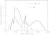 |
Fig. B.2 Same as in Fig. B.1, but contributions to the force multiplier counted inside 50 Å wide bands are shown as a function of wavelength. |
Figure B.4 shows the change in the force multiplier as a function of the number of photons in the radiator between 100 and 230 Å (relative to that of a 125 000 K blackbody). The plot shows curves for several (log(ξ), log(t)) pairs. Decreasing ξ or t enhances the line force. Fig. B.5 shows some spectral energy distributions for the radiators of the intermediate spectral state at Φ = 0 (along the line joining the centers of components) and some examples of partially cut blackbodies with which force multiplier grids were computed. At each wind layer, the coadded number of photons (from WR and compact star) between 100 and 230 Å was computed and the force multiplier was interpolated from a precomputed grid.
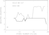 |
Fig. B.3 Mean ionization (weighted by the contribution to the force multiplier) as a function of atomic number shown for log(ξ) = 2.5 and log(t) = −1.84 (as in Figs. B.1 and B.2). |
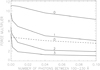 |
Fig. B.4 Force multiplier vs. the number of photons in the radiator between 100 and 230 Å (in units of that in 125 000 K blackbody). Curves for four log(ξ)-values (0, 1, 2, 3) with log(t) = −1.85 are plotted (solid lines). The dashed line is for the (log(ξ), log(t))-pair (0,−1.36). |
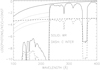 |
Fig. B.5 Spectral energy distributions for the radiators of the intermediate spectral state at Φ = 0 (along the line joining the centers of components). Solid lines show the WR spectra at the photosphere (125 000 K blackbody) and the absorbed spectra at distance 2 RWR from the WR surface. The dashed lines show the compact star spectra (unabsorbed and absorbed at distance 0.1 RWR from the WR surface). The dotted lines show some partially cut blackbodies used to compute force multiplier grids. |
Appendix C Comparison of our method (XSTAR) and CMF methods
C.1 OB-star winds
Krticka & Kubat (2017) computed comoving frame winds (CMF) for a model grid of O stars comprising main-sequence stars, giants, and supergiants (their Table 1). Using the masses, radii, effective temperatures, and solar chemical abundances (Asplund et al. 2009), we computed the wind models with the XSTAR method. The data were reproduced from extensive computations in Vilhu & Kallman (2019). The wind equations were integrated numerically, resulting in velocity stratification v(r) that was compared with the widely used β-velocity model,
![Mathematical equation: \begin{eqnarray*} v_{\textrm{model}} &=& v_{\mathrm{{inf}}}(1 - B/x)^{\beta} \\[10pt] B &=& 1. - (v_{\textrm{in}}/v_{\textrm{inf}})^{1/\beta} \\[10pt] x &=& r/R_{\textrm{star}}. \end{eqnarray*}](/articles/aa/full_html/2021/05/aa40620-21/aa40620-21-eq20.png)
The integrations were started above the subsonic region at x = 1.01 and ended at x = 10, using 1000 grid points with δx = 0.01. The subsonic part of the wind enters only through the boundary condition vin = 10 km s−1 (at x = 1.0). The resulting v(x) was then compared with the model vmodel(x). The unknown free parameters mass-loss rate Mdot and vinf (velocity at infinity) were iterated using the IDL procedure mpcurvefit.pro (written by Craig Markwardt) to obtain (v(x) − vmodel(x))/vmodel(x) to approach zero at each x. The procedure mpcurvefit.pro performs a Levenberg-Marquardt least-squares fit, and no weighting was used. Density clumping was not used by either Krticka & Kubat (2017) or here. The formal one-sigma errors of each parameter were computed from the covariance matrix.
β was set to 0.6, giving overall the best-fitting results. Using β = 1.0, Ṁ and vinf should be multiplied on average by 0.7 and 1.4, respectively (see details in Vilhu & Kallman 2019). Figure C.1 compares our XSTAR models and the CMF models. Increasing β from 0.6 to 0.8 would give better agreement at high mass-loss rates. However, the overall agreement is moderately good.
C.2 X-ray contaminated wind of Vela X-1
Krticka et al. (2012) applied the CMF method to the X-ray contaminated wind of Vela X-1 pulsar. This is a binary system with an orbital period of 8.96 days and a separation of 53.4 R⊙. The masses of the neutron star and of the companion O star are 1.88 and 23.5 solar masses, respectively. The O star has an effective temperature of 27 000 K and a radius 30 R⊙, and the wind mass-loss rate is 1.5 × 10⁻⁶ M⊙ yr−1. The X-ray luminosity of the neutron star 3.5 × 1036 erg s−1 was assumed with a photon index Γ = 1 (Watanabe et al. 2006). Force multiplier grids with different EUV contaminations were computed for the 27 000 K blackbody in a similar fashion as explained for Cyg X-3 (Appendix B). In the Vela X-1 case, the number of EUV photons relative to that of 27 000 K blackbody is larger than 1. The geometry is illustrated in Fig. 1 of Krticka et al. (2012).
Our method was applied to Vela X-1 in a similar fashion as to Cyg X-3. Fig. C.2 shows the computed velocity stratifications for different orbital angles Φ. The trend is similar to that in Krticka et al. (2012, their Fig. 3, reproduced here as Fig. C.3). Our study gives a weaker Φ-dependence, but the results are qualitatively similar. Quantitative differences are expected because the approaches are very different.
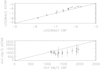 |
Fig. C.1 Comparison of CMF models of Krticka & Kubat (2017) with XSTAR models of our study. M⊙ (solar masses yr−1) and vinf (km s−1) are the mass-loss rate and velocity at infinity, respectively. |
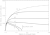 |
Fig. C.2 Radial wind velocity stratifications of Vela X-1 for different orbital angles Φ marked (0–90 degrees). The label ‘NO X’ shows the wind without X-rays from the neutron star at radius 1.78. The radius is measured from the center of the O star in units of 30 R⊙ (= O-star radius). |
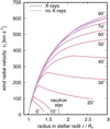 |
Fig. C.3 Related Vela X-1 study reproduced from Krticka et al. (2012). Radial wind velocity stratifications for different orbital angles Φ. The position of the neutron star is marked in the graph. |
References
- Abbott, D. C. 1982, ApJ, 259, 282. [NASA ADS] [CrossRef] [Google Scholar]
- Antokhin, I. I., & Cherepashchuk, A. M. 2019, ApJ, 871, 244. [Google Scholar]
- Asplund, M., Grevesse, N., Sauval, A. J., & Scott, P. 2009, ARA&A, 47, 481 [NASA ADS] [CrossRef] [Google Scholar]
- Castor, J. I., Abbott, D. C., & Klein, R. I. 1975, ApJ, 195, 157 [NASA ADS] [CrossRef] [Google Scholar]
- Coppi, P. 1992 MNRAS, 258, 657 [NASA ADS] [CrossRef] [Google Scholar]
- El Hassan, N., Bizau, C., Blancard, P., et al. 2009, Phys. Rev., A79, 033415 [Google Scholar]
- Ergma, E., & Yungelson, L. R. 1998, A&A, 333, 151. [Google Scholar]
- Frank, J., King, A., & Raine, D. 1992, Accretion Power in Astrophysics, Cambridge Astrophysics Series 21, 2nd edn. (Cambridge: Cambridge University Press) [Google Scholar]
- Gayley, K. G., Owocki, S. P. & Cranmer, S. R. 1995, ApJ, 442, 296. [NASA ADS] [CrossRef] [Google Scholar]
- Giacconi, R., Gorenstein, P., Gursky, H. & Waters, J. P. 1967, ApJ, 148, L119. [NASA ADS] [CrossRef] [Google Scholar]
- Grassitelli, L., Langer, N., Grin, N. J., et al. 2018, A&A, 614, A86 [NASA ADS] [CrossRef] [EDP Sciences] [Google Scholar]
- Hainich, R., Ruhling, U., Todt, H., et al. 2014, A&A, 565, A27 [NASA ADS] [CrossRef] [EDP Sciences] [Google Scholar]
- Hamann, W.-R., & Koesterke, L. 1998, A&A, 335, 1003 [NASA ADS] [Google Scholar]
- Hamann, W.-R., Koesterke, L., & Wessolowski, U. 1995, A&A, 299, 151 [NASA ADS] [Google Scholar]
- Hamann, W.-R., Gräfener, G., & Liermann, A. 2006, A&A, 457, 1015 [NASA ADS] [CrossRef] [EDP Sciences] [Google Scholar]
- Hanson, M. M., Still, M. D., & Fender, R. P. 2000, ApJ, 541, 308 [NASA ADS] [CrossRef] [Google Scholar]
- Hjalmarsdotter, L., Zdziarski, A. A., Szostek, S., & Hannikainen, D. C. 2009, MNRAS, 392, 251. [NASA ADS] [CrossRef] [Google Scholar]
- Hubeny, I., Parland, G., & Wolf, Savin, D. 2001, ASP Conf. Ser., 247 [Google Scholar]
- Kallman, T. R. 2018, XSTAR. A Spectral Analysis Tool, version 2.5. NASA, Goddard Space Flight Center, December 14, 2018 [Google Scholar]
- Kallman, T. R., McCollough, M., Koljonen, K., et al. 2019, ApJ, 874, 51 [CrossRef] [Google Scholar]
- Karino, S. 2014, PASJ, 66, 34 [NASA ADS] [Google Scholar]
- Karino, S., Nakamura, K., & Taani, A. 2019, PASJ, 71, 58 [Google Scholar]
- Koljonen, K. I. I., & Maccarone, T. J. 2017, MNRAS, 472, 78 [NASA ADS] [CrossRef] [Google Scholar]
- Krticka, J., & Kubat, J. 2017, A&A, 606, A31 [NASA ADS] [CrossRef] [EDP Sciences] [Google Scholar]
- Krticka, J., Kubat, J., & Skalicky, J. 2012, ApJ, 757, 162 [NASA ADS] [CrossRef] [Google Scholar]
- Krticka, J., Kubat, J., & Krtickova, I. 2018, A&A, 620, A150 [NASA ADS] [CrossRef] [EDP Sciences] [Google Scholar]
- Liu, Q. R., van Paradijs, J., & van den Heuvel, E. P. J. 2006, A&A, 455, 1165 [NASA ADS] [CrossRef] [EDP Sciences] [Google Scholar]
- MacGregor, K. B., & Vitello, P. A. J. 1982, ApJ, 259, 267 [NASA ADS] [CrossRef] [Google Scholar]
- Martinez-Nunez, S., Kretchmar, P., Borzo, E. et al. 2017, Space Sci. Rev., 212, 59. [NASA ADS] [CrossRef] [Google Scholar]
- McCollough, M., Corrales, L., & Dunham, M. M. 2016, ApJ, 830, L36 [NASA ADS] [CrossRef] [Google Scholar]
- Meyer-Hofmeister, E., Liu, B. F., Qiao, E., & Taam, R. E. 2020, A&A, 637, A66 [EDP Sciences] [Google Scholar]
- Mewe, R., & Schrijver, J. 1978, A&A, 65, 99 [NASA ADS] [Google Scholar]
- Nugis, T., & Lamers, H. J. G. L. M. 2000, A&A, 360, 227 [NASA ADS] [Google Scholar]
- Sander, A. A. C., Hamann, W.-R., Todt, H., Hainich, R. & Shenar, T. 2017, A&A, 603, A86 [NASA ADS] [CrossRef] [EDP Sciences] [Google Scholar]
- Sander, A. A. C., Furst, F., Kretchmar, P., et al. 2018, A&A, 610, A60 [NASA ADS] [CrossRef] [EDP Sciences] [Google Scholar]
- Szostek, A., & Zdziarski, A. A. 2008, MNRAS, 386, 593 [NASA ADS] [CrossRef] [Google Scholar]
- Stevens, I. R.,& Kallman, T. R. 1990, ApJ, 365, 321 [NASA ADS] [CrossRef] [Google Scholar]
- Sundqvist, J. O., Puls, J., & Feldmeier, A. 2010, A&A, 510, A11 [NASA ADS] [CrossRef] [EDP Sciences] [Google Scholar]
- Sundqvist, J. O., Puls, J., & Owocki, S. P. 2014, A&A, 568, A59 [NASA ADS] [CrossRef] [EDP Sciences] [Google Scholar]
- van Keerkwijk, H. M., Charles, P. A., Geballe, T. R., et al. 1992, Nature, 355, 703 [NASA ADS] [CrossRef] [Google Scholar]
- van Keerkwijk, H. M., Geballe, T. R., King, D. L., van der Klis, M., & van Paradijs, J. 1996, A&A, 314, 521 [Google Scholar]
- Vilhu, O., & Kallman, T. R. 2019, ArXiv eprints: [arXiv:1906.05581v1] [Google Scholar]
- Vilhu, O., Hakala, P., Hannikainen, D. C., McCollough, M., & Koljonen, K. 2009, A&A, 501, 569 [Google Scholar]
- Vilhu, O., Hjalmarsdotter, L., Zdziarski, A. A., et al. 2003, A&A, 411, L405 [NASA ADS] [CrossRef] [EDP Sciences] [Google Scholar]
- Watanabe, S., Sako, M., Ishida, M., et al. 2006, ApJ, 651, 421 [Google Scholar]
- Zdziarski, A. A., Mikolajewska, J., & Belczynski, K. 2013, MNRAS, 429, L104 [NASA ADS] [CrossRef] [Google Scholar]
- Zdziarski, A. A., Segreto, A., & Pooley, G. G. 2016, MNRAS, 456, 775 [NASA ADS] [CrossRef] [Google Scholar]
- Ziolkowski, J., & Zdziarski, A. A. 2018, MNRAS, 480, 1580 [NASA ADS] [CrossRef] [Google Scholar]
All Tables
Luminosities and EUV-fluxes of the five basic states of Cyg X-3 from RXTE observations and EQPAIR models (Hjalmarsdotter et al. 2009, first two rows) and computed wind velocities at the compact star (this study, last rows).
All Figures
|
Fig. 1 Unabsorbed model spectra of the five main accretion states of Cyg X-3 reproduced from Hjalmarsdotter et al. (2009). The models corresponding to the hard state (solid blue line), the intermediate state (long-dashed cyan line), the very high state (short-dashed magenta line), the soft nonthermal state (dot-dashed green line), and the ultrasoft state (dotted red line) are shown (unabsorbed at Earth). |
| In the text | |
|
Fig. 2 Number of photons between 100 and 230 Å (in units of that from a 125 000 K blackbody) as a function of the distance from the WR star surface (the intermediate model of Table A.1 (fvol = 0.3, Φ = 0) along the line joining the stars). The compact star is located at 2.4 RWR. The solid line shows the contribution from the WR star and the dashed line that from the compact star (X-ray source). The dotted line shows the coadded contribution. |
| In the text | |
|
Fig. 3 Geometry of the system in the orbital plane in units of the WR star radius. The compact star (CS) is located at distance 3.4 from the center of the WR star. The orbital angle Φ (PHI) is marked in the direction of the motion of the compact star. |
| In the text | |
|
Fig. 4 Left panel: computed wind velocities as a function of the radial distance from the center of the WR star (in units of stellar radius) for the orbital angle Φ = 0 deg (solid lines, see Fig. 3). The clumping volume filling factor f = fvol = 0.3. VH = very high state, INT = intermediate state, HARD = hard state, and NOX = the wind without X-rays from the compact star (whose distance is marked as CS in the plot). Dashed lines are for the intermediate state for angles Φ = 30 deg (lower) and 90 deg (upper). Right panel: wind radial velocities for the very high state with three clumping volume filling factors f = fvol = 1.0, 0.3, and 0.1 (dashed lines). The solid line shows the wind without X-rays (NOX) and with f = 0.3. The gravitational pull of the compact star is not included. |
| In the text | |
|
Fig. 5 Left panel: computed accretion luminosities (in units of 1038 erg s−1) for thefive spectral states of Cyg X-3 are shown for three clumping filling factors f = fvol = 1.0 (dotted lines), = 0.3 (dashed lines), and = 0.1 (solid lines). The orbital angle Φ = 0 deg for the upper curves and Φ = 30 deg for the lower ones. The filled squares show the EQPAIR model luminosities (Lbol of Table A.1) The compact star mass is 2.4 M⊙. In the abscissa 0 indicates NOX (no X-rays), 1 hard, 2 soft nonthermal, 3 intermediate, 4 ultrasoft, and 5 very high state. Right panel: same as in the left panel, but the compact star mass is 3.0 M⊙. |
| In the text | |
|
Fig. B.1 Contributions to the force multiplier (FM) as a function of the element atomic number (26 for Fe). A 135 000 K blackbody (dashed line) and below 230 Å totally cut blackbody (Nphot = 0 between 100 and 230 Å) with the same temperature (solid line) were used as radiators, and the force multiplier was calculated at log(ξ) = 2.5 and log(t) = −1.84. The y-axis has a logarithmic scale. |
| In the text | |
|
Fig. B.2 Same as in Fig. B.1, but contributions to the force multiplier counted inside 50 Å wide bands are shown as a function of wavelength. |
| In the text | |
|
Fig. B.3 Mean ionization (weighted by the contribution to the force multiplier) as a function of atomic number shown for log(ξ) = 2.5 and log(t) = −1.84 (as in Figs. B.1 and B.2). |
| In the text | |
|
Fig. B.4 Force multiplier vs. the number of photons in the radiator between 100 and 230 Å (in units of that in 125 000 K blackbody). Curves for four log(ξ)-values (0, 1, 2, 3) with log(t) = −1.85 are plotted (solid lines). The dashed line is for the (log(ξ), log(t))-pair (0,−1.36). |
| In the text | |
|
Fig. B.5 Spectral energy distributions for the radiators of the intermediate spectral state at Φ = 0 (along the line joining the centers of components). Solid lines show the WR spectra at the photosphere (125 000 K blackbody) and the absorbed spectra at distance 2 RWR from the WR surface. The dashed lines show the compact star spectra (unabsorbed and absorbed at distance 0.1 RWR from the WR surface). The dotted lines show some partially cut blackbodies used to compute force multiplier grids. |
| In the text | |
|
Fig. C.1 Comparison of CMF models of Krticka & Kubat (2017) with XSTAR models of our study. M⊙ (solar masses yr−1) and vinf (km s−1) are the mass-loss rate and velocity at infinity, respectively. |
| In the text | |
|
Fig. C.2 Radial wind velocity stratifications of Vela X-1 for different orbital angles Φ marked (0–90 degrees). The label ‘NO X’ shows the wind without X-rays from the neutron star at radius 1.78. The radius is measured from the center of the O star in units of 30 R⊙ (= O-star radius). |
| In the text | |
|
Fig. C.3 Related Vela X-1 study reproduced from Krticka et al. (2012). Radial wind velocity stratifications for different orbital angles Φ. The position of the neutron star is marked in the graph. |
| In the text | |
Current usage metrics show cumulative count of Article Views (full-text article views including HTML views, PDF and ePub downloads, according to the available data) and Abstracts Views on Vision4Press platform.
Data correspond to usage on the plateform after 2015. The current usage metrics is available 48-96 hours after online publication and is updated daily on week days.
Initial download of the metrics may take a while.