| Issue |
A&A
Volume 649, May 2021
|
|
|---|---|---|
| Article Number | A138 | |
| Number of page(s) | 10 | |
| Section | Galactic structure, stellar clusters and populations | |
| DOI | https://doi.org/10.1051/0004-6361/202140574 | |
| Published online | 28 May 2021 | |
Properties of the brightest globular cluster in M 81 based on multicolour observations⋆
1
Key Laboratory of Optical Astronomy, National Astronomical Observatories, Chinese Academy of Sciences, Beijing 100012, PR China
e-mail: This email address is being protected from spambots. You need JavaScript enabled to view it.
, This email address is being protected from spambots. You need JavaScript enabled to view it.
2
School of Astronomy and Space Sciences, University of Chinese Academy of Sciences, Beijing 100049, PR China
Received:
16
February
2021
Accepted:
9
March
2021
Abstract
Context. Researching the properties of the brightest globular cluster (referred to as GC1) in M 81 can provide a fossil record of the earliest stages of galaxy formation and evolution. The Beijing–Arizona–Taiwan–Connecticut (BATC) Multicolour Sky Survey has carried out deep exposures of M 81.
Aims. We derive the magnitudes in intermediate-band filters of the BATC system for GC1 and determine its age, mass, and structural parameters.
Methods. GC1 was observed by BATC using 14 intermediate-band filters covering a wavelength range of 4000–10 000 Å. Based on photometric data in BATC and Two Micron All Sky Survey near-infrared JHKs filters, we constructed an extensive spectral energy distribution of GC1, spanning the wavelength range from 4000 to 20 000 Å. By comparing multicolour photometry with theoretical single stellar population synthesis models, we derived the age and mass of GC1. In addition, we obtained ellipticities, position angles, and surface brightness profiles for GC1 based on the images of deep observations with the Advanced Camera for Surveys on the Hubble Space Telescope. GC1 is better fitted by the Wilson model than by the King and Sérsic models in the F606W filter, and it is better fitted by the Sérsic model than by the King and Wilson models in the F814W filter. The ‘best-fit’ half-light radius of GC1 obtained here is 5.59 pc, which is larger than the majority of normal globular clusters (GCs) of the same luminosity.
Results. The age and mass of GC1 estimated here are 13.0 ± 2.90 Gyr and 1.06 − 1.48 × 10⁷ M⊙, respectively. The Rh versus MV diagram shows that GC1 occupies the same area as extended star clusters. Therefore, we suggest that GC1 is more likely an accreted former nuclear star cluster than a classical GC similar to most of those in the Milky Way.
Key words: galaxies: evolution / galaxies: star clusters: individual: globular cluster
Full Table 4 is only available at the CDS via anonymous ftp to cdsarc.u-strasbg.fr (130.79.128.5) or via http://cdsarc.u-strasbg.fr/viz-bin/cat/J/A+A/649/ A138
© ESO 2021
1. Introduction
From both a stellar population and stellar dynamics point of view, globular clusters demonstrate a very interesting family of stellar systems (Meylan et al. 2001). They are among the oldest bound stellar systems in the Universe and can provide a fossil record of the earliest stages of galaxy formation and evolution. In addition, studying the spatial structures and internal stellar kinematics of GCs can help us understand both their formation conditions and dynamical evolution within the tidal fields of their galaxies (Brodie & Strader 2006; Barmby et al. 2007; Forbes et al. 2018).
Beasley et al. (2002) investigated the formation of GC systems of elliptical galaxies within the framework of a semianalytic model of galaxy formation. These authors could reproduce the observed bimodal colour distributions by assuming that GCs were formed at high redshifts (z > 5) in protogalactic fragments, and during the subsequent gas-rich merging of these fragments. West et al. (2004) raised the idea that GCs can aid in probing a galaxy environment on different timescales from the earliest epoch of formation to the most recent merging events. Recent works have shown that the simple assumption that GCs form in intense star-forming episodes can lead self-consistently to many of the observed properties of GC systems at the present day (see Li & Gnedin 2014; Kruijssen 2015; Pfeffer et al. 2018, and references therein). However, Brodie & Strader (2006) pointed out a relationship between the classic scenarios of in situ formation in a large protogalaxy (Forbes et al. 1997), major mergers (Ashman & Zepf 1992), and minor mergers (Côté et al. 1998); also, the ‘biased hierarchical merging’ (Beasley et al. 2002) compromises it, indicating that these three scenarios are hard to distinguish from one another at a high redshift. In order to gain better insight into the details of just how galaxies come together, as well as why their GC populations show the trends that they do with galaxy mass and morphology and yet seem to have an almost universal luminosity function despite these differences (see Hanes 1977a,b; Harris 1991, and references therein), the study of GCs in a wide variety of external galaxies is useful.
As far as very bright and massive GCs are concerned, their connection to nuclear star clusters (NSCs) of low-mass galaxies, and thus their connection to accretion scenarios (‘galactic cannibalism’), is of particular interest. In the Milky Way, some of the most massive GCs exhibit clear spreads in [Fe/H] (see Villanova et al. 2014; Johnson et al. 2020, and the introduction of Sakari et al. 2021). The fact that they were once the NSCs of dwarf galaxies which have since been accreted into the Milky Way may explain the iron-complex GCs. Antonini et al. (2015) studied the evolution of NSCs in a cosmological context by taking into account the growth of NSCs due to both in situ formation at the galactic centre from infalling gas and the migration of stellar clusters to the centre. These authors found that in situ star formation contributes a significant fraction (up to ∼80%) of the total mass of NSCs, and that both NSC growth through in situ star formation and that through star cluster migration can generate NSCs. However, there is also some potential evidence against this scenario for certain high-mass GCs, as Sakari et al. (2021) show that G1, one of the most massive star clusters in M31, resembles that of what are thought to be in situ M31 GCs by the detailed chemical analysis. These authors show that G1’s chemical properties are found to resemble other M31 GCs, though it also shares some similarities with extragalactic NSCs.
M 81 is the nearest large spiral galaxy outside the Local Group, and its GCs are an important target of study. As such, its GC system has come under recent detailed scrutiny. Perelmuter & Racine (1995) first attempted to identify GCs in M 81 from ground-based images. However, at the distance of M 81, the diameters of GCs are typically comparable to the seeing disk, and it is difficult to recognise GCs on the basis of image structure from ground-based observation. So, before 2001, there are only a few papers that studied the GCs in M 81 (see Schroder et al. 2002, and references therein). Since the pioneering work of Chandar et al. (2001), the era of detecting and studying M 81 GCs based on the images taken with the Hubble Space Telescope (HST) has begun (Chandar et al. 2001; Nantais et al. 2010; Santiago-Cortés et al. 2010). In a systematic search for compact clusters in M 81 using the images observed with the Advanced Camera for Surveys on the HST, Santiago-Cortés et al. (2010) identified the brightest GC in M 81, GC1 (the nomenclature introduced by Mayya et al. 2013). As the brightest GC in M 81, GC1 has attracted much scientific interest (see, e.g., Mayya et al. 2013, and references therein). GC1 appears to be a peculiar case, given that Mayya et al. (2013) present that it has a high metallicity, a short star formation history, and a disk-like radial velocity (suggestive of a thick-disk in situ GC), while its mass, size, and shape are more consistent with a former NSC. Although Mayya et al. (2013) argue that GC1 was, nonetheless, still a probable former NSC, these other data possibly point to a biased hierarchical merging scenario in which this cluster was near the core of a relatively massive protogalaxy that merged with the proto-M 81 main disk quite early.
Due to their proximity, galaxies in the Local Group provide us with ideal targets for detailed studies of spatial structures and dynamics of GCs. The GCs of the Milky Way, M 31 and M 33, have received close attention (see McLaughlin & van der Marel 2005; Wang & Ma 2013; Ma 2015, and references therein). Beyond the Local Group, the detailed studies of spatial structures and dynamics of the GC system in NGC 5128, the central giant elliptical in the Centaurus group, has also received close attention (see McLaughlin et al. 2008; Taylor et al. 2010, and references therein). However, at the nearly equal distance with NGC 5128 from us, structural and dynamical studies of individual clusters in the GC system of M 81 are very limited. Mayya et al. (2013) determined structural parameters for GC1 in M 81 by fitting the empirical King model (King 1962) to the internal surface brightness of the HST images. Ma et al. (2017) determined structural and dynamical parameters for two GCs in the remote halo of M 81 and M 82 in the M 81 group by fitting three models to the internal surface brightness of the HST images.
Since the pioneer work of McLaughlin & van der Marel (2005), three models, which were developed by King (1966), Wilson (1975), and Sérsic (1968), have been frequently used in the fits. Using the three models, some authors have achieved some success in determining structural and dynamical parameters of clusters in the Local galaxies: the Milky Way, the Large and Small Magellanic Clouds, Fornax and Sagittarius dwarf spheroidal galaxies (McLaughlin & van der Marel 2005), M 31 (Barmby et al. 2007, 2009; Wang & Ma 2013), NGC 5128 (McLaughlin et al. 2008), M 33 (Ma 2015), and the M 81 group (Ma et al. 2017).
Mayya et al. (2013) have studied GC1 in detail based on the multi-band photometric and optical spectroscopic data. They derived the metallicity, age, and mass of GC1. And these authors also obtained the core radius, tidal radius, and half-light radius of GC1. Our results may provide more insight as to the nature of this cluster and its implications for the role of accretion of dwarf satellites in the formation of M 81 and similar massive galaxies. In addition, we want to say that the research on structural properties here is newer, and that our main innovation is the use of multiple models and choosing the best in each of our images.
Unlike previous studies on this cluster, in this paper, we fit multiple models for the structural and dynamical parameters and choose the best fits, and we estimate the age and mass using a smaller total range of wavelengths. We describe the details of the observations and our approach to the data reduction with the BATC system and the HST in Sects. 2 and 4. We estimate the age and mass of GC1 by comparing observational spectral energy distributions (SEDs) with population synthesis models in Sect. 3 and determine structural and dynamical parameters of GC1 in Sect. 5. We provide a summary in Sect. 6. The distance is considered to be (m − M)0 = 27.80 ± 0.08 to M 81 throughout, which is from Durrell et al. (2010).
2. Archival images of the BATC multicolour sky survey and 2MASS
We have obtained deep exposures of the M 81 using the multicolour wide-field BATC survey system (Fan et al. 1996; Zhou et al. 2001). The BATC observing system uses a 15 intermediate-band filter system across the whole optical spectrum accessible from the ground with filter bandwidths ranging from 25 to 35 nm and avoids the strong night-sky emission lines (Yan et al. 2000). The BATC system is mounted at the 60/90 cm Schmidt telescope at the Xinglong Station of the National Astronomical Observatories, Chinese Academy of Sciences. Our observations cover a wavelength range of 389–1000 nm using the 14 filters, with a total exposure time of ∼100 h from 1995 to 2002. For flux calibration, the Oke-Gunn (Oke & Gunn 1983) primary flux standard stars HD 19445, HD 84937, BD +26°2606, and BD +17°4708 were observed during photometric nights (Yan et al. 2000).
We performed all of the reduction for the CCD images with standard procedures including bias subtraction and flat fielding (Fan et al. 1996; Zheng et al. 1999). In order to improve the signal-to-noise ratios (S/Ns), we combined multiple images of the same filter to one using the BATC-specific algorithm (Zhou et al. 2003). Zhou et al. (2003) showed that the cosmic ray hits and bad pixels were corrected through a comparison of multiple images when combining the images. Before the combination, the images were shifted and rotated according to the precise locations of stars in the HST Guide Star Catalogue (GSC; Jenkner et al. 1990). Also, we did photometry in the combined images. Calibration of the magnitude zero level in the BATC photometric system is similar to that of the spectrophotometric AB magnitude system. We performed standard aperture photometry of GC1 using the PHOT routine in DAOPHOT (Stetson 1987). To ensure that we adopted the most appropriate photometric radius (Rap) that encloses all light from GC1, we produced a curve of growth from the g-band photometry obtained through apertures with radii in the range of 2–11 pixel with 1 pixel increments. The local sky background was measured in an annulus with an inner radius of Rap + 1 pixels and a width of 5 pixels. The finding chart of GC1 observed in the BATC g-band and the final photometric radius are shown in Fig. 1. Figure 1 also plots the image of GC1 observed in the F606W filter of ACS/HST. Finally, we determined photometry for GC1 in the individual 14 intermediate-band filters. Table 1 lists the BATC photometry of GC1, with errors given by IRAF/DAOPHOT.
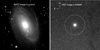 |
Fig. 1. Left panel: image of GC1 in the BATC g band obtained with the 60/90 cm Schmidt telescope in the BATC Multicolour Sky Survey, of which the circle is photometric aperture adopted in this paper. Right panel: image of GC1 observed in the F606W filter of ACS/HST, of which the circle around GC1 is of a 6 arcsec radius. |
BATC and 2MASS photometry of GC1 in M 81.
Some works showed that the age-metallicity degeneracy can be partially broken by adding NIR photometry to the optical colours (see Ma et al. 2009, and references therein). In order to derive the age and mass of GC1 accurately, we used the photometry in the JHKs bands. In addition, although Kaviraj et al. (2007) showed that the combination of far and near-ultraviolet (NUV) photometry with optical observations in the standard broad bands can efficiently break the age-metallicity degeneracy, Mayya et al. (2013) show an ultraviolet (UV) excess for GC1. These authors give advice not to use UV fluxes to derive the age and metallicity of an old simple population by fitting spectral energy distributions (SEDs). Mayya et al. (2013) guessed the age of GC1 to be older than 13 Gyr by comparing multicolour photometry with the multiple stellar generation model including the He-rich population with blue horizontal branch stars. So, in this paper, we do not use the UV photometry in the GALEX to derive the age of GC1.
We used the 2MASS archival images of M 81 in the JHKs bands to do photometry. The images were retrieved using the 2MASS Batch Image Service1. The reason why we used 2MASS is that there is the lack of need for better depth or resolution of newer NIR imaging given the properties of GC1. In addition, we consider that the quality of the photometric and astrometric calibrations of the 2MASS system is adequate for our science goals. The uncompressed atlas images were used with a resampled spatial resolution of ∼1 arcsec pixel−1. We also performed standard aperture photometry of GC1 on the images in the JHKs bands using the PHOT routine in DAOPHOT. To determine the total luminosity of GC1, we produced a curve of growth from the J-band photometry obtained through apertures with radii in the range of 3–14 pixel with 1 pixel increments. Then, the most appropriate photometric radius from the curve of growth that encloses the total light of GC1 was obtained. GC1 is projected onto the M 81 disk, the background around it is highly variable. So, in order to obtain the light of GC1 correctly, the local sky background was measured in an annulus with an inner radius 1 pixel larger than the photometric radius and 5 pixels wide. Finally, the instrumental magnitudes were then calibrated using the relevant zero points obtained from the photometric header keywords of each image. Table 1 lists the 2MASS photometry of GC1, with errors given by IRAF/DAOPHOT.
3. Stellar populations of GC1 in M 81
3.1. Metallicity and reddening value of GC1
It is well known that the SEDs of GCs are determined by the combination of their ages and metallicities, which is often described as the age-metallicity degeneracy. Therefore, the age of a cluster can only be obtained accurately if the metallicity is from independent determinations with confidence. There exist two metallicity determinations for GC1, one is [Fe/H] = −0.86 ± 0.41 which was determined by Nantais & Huchra (2010) and the other is −0.6 ± 0.10 which was determined by Mayya et al. (2013). Nantais & Huchra (2010) observed the spectra for 74 M 81 GCs including GC1, with Hectospec on the 6.5 m MMT on Mt. Hopkins in Arizona, and they determined the metallicities for these GCs. Mayya et al. (2013) derived the metalicity of GC1 based on the spectroscopic observations using the long-slit of the spectrograph of the OSIRIS instrument at the 10.4 m GTC. The metallicity obtained by Mayya et al. (2013) is based on a higher S/N spectrum on a higher-resolution spectrograph, and it specifically used iron lines rather than a mix of spectral indices linked to different chemical elements (and originally optimised for low-resolution spectroscopy). So, here we adopted the value of metallicity from Mayya et al. (2013). In addition, in order to obtain intrinsic SEDs of GC1, the photometry must be corrected for reddening from the foreground extinction contribution of the Milky Way and for the internal reddening due to varying optical paths through the disk of M 81. The total reddening in M 81 (foreground plus M 81 contribution) has been measured by a number of authors (e.g., Freedman et al. 1994; Kong et al. 2000). Here, we only mention that Kong et al. (2000) obtained the reddening maps of M 81 based on the images in 13 intermediate-band filters from 3800 to 10 000 Å. To determine the metallicity, age, and reddening distributions for M 81, Kong et al. (2000) found the best match between the observed colours and the predictions from the single stellar population (SSP) models. A map of the interstellar reddening in a substantial portion of M 81 were obtained. We used the reddening data of Kong et al. (2000) which is E(B − V) = 0.09 for GC1. In fact, Mayya et al. (2013) also used E(B − V) = 0.09 as the reddening value for GC1.
3.2. Stellar populations and synthetic photometry
We determined the age and mass of GC1 in M 81 by comparing its SEDs with theoretical stellar population-synthesis models. The SEDs of GC1 include the photometric data in 14 BATC intermediate-band and 2MASS near-infrared (NIR) JHKs filters obtained in Sect. 2. The theoretical stellar population-synthesis models we use in this paper are the GALEV SSP models (e.g., Kurth et al. 1999; Schulz et al. 2002; Anders & Fritze-v. Alvensleben 2003).
We convolved the theoretical SSP SEDs of GALEV with the BATC b − p and 2MASS JHKs filter response curves to obtain synthetic optical and NIR photometry, which were computed by
 (1)
(1)
where Fλ is the theoretical SED which varies with age and metallicity, and φi is the response function of the ith filter of the BATC and 2MASS photometric systems.
3.3. Age
We used a χ2 minimisation approach to obtain the best fit between SEDs of SSP models and the intrinsic SEDs of GC1, following
![Mathematical equation: $$ \begin{aligned} \chi ^2=\sum _{i=1}^{N}{\frac{[m_{\lambda _i}^\mathrm{intr}-m_{\lambda _i}^\mathrm{mod}(t)]^2}{\sigma _{i}^{2}}}, \end{aligned} $$](/articles/aa/full_html/2021/05/aa40574-21/aa40574-21-eq2.gif) (2)
(2)
where  is the integrated magnitude in the ith filter of a theoretical SSP at age
  represents the intrinsic integrated magnitude in the same filter, and σi is the magnitude uncertainty, defined as
 (3)
(3)
Here, σobs, i is the observational uncertainty from Table 1 of this paper, σmod, i is the uncertainty associated with the model itself, and σmd, i is associated with the uncertainty with the distance modulus adopted here. Following Ma et al. (2012), we adopt σmod, i = 0.05 mag. For σmd, i, we adopt 0.08 from Durrell et al. (2010). Furthermore, N is the number of photometries used in the fitting.
Before fitting, we obtained the theoretical SEDs for the metallicity [Fe/H] = −0.6 model by interpolation of between [Fe/H] = −0.64 and −0.33 models for GC1, and the values for the extinction coefficient, Rλ, were obtained by interpolating the interstellar extinction curve of Cardelli et al. (1989). In the end, we obtained the age of GC1 to be 13.0 ± 2.90 Gyr. We present the results of fittings for GC1 in Fig. 2.
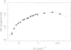 |
Fig. 2. Best-fitting, integrated theoretical GALEV SEDs compared to the intrinsic SEDs of GC1. The photometric measurements are shown as symbols with error bars (vertical error bars for photometric uncertainties and horizontal ones for the approximate wavelength coverage of each filter). The open circles represent the calculated magnitudes of the model SED for each filter. |
Mayya et al. (2013) calculated a new set of SSP models including an enhanced value of initial He content which can fit the UV excess very well. These authors obtained the age of GC1 to be ≥13.0 Gyr, which is in agreement with the age obtained here.
3.4. Mass
In this section, we determine the mass of GC1. The GALEV models provide absolute magnitudes (in the Vega system) in 77 filters for SSPs of 106M⊙, which includes Johnson UBVRI (for details, see Landolt 1983), Cousins RI (for details, see Landolt 1983), and JHK (Bessell & Brett 1988) systems. We obtained the mass of GC1 by using the difference between the intrinsic absolute magnitudes and those given by the models in units of 106M⊙. To reduce mass uncertainties resulting from photometric uncertainties based on only magnitudes in one filter (in general the V band is used), we determined the mass of GC1 using magnitudes in the UBVRI and JHKs bands. Zhou et al. (2003) derived the relationships between the BATC intermediate-band system and the broad-band system. The magnitudes in the BVRI bands were obtained using the photometries of the BATC intermediate-band system here, which are mB = 17.60 ± 0.030, mV = 16.70 ± 0.023, mR = 16.37 ± 0.026, and mI = 15.38 ± 0.004. In addition, we transformed the 2MASS JHKs magnitudes to the photometric system of Bessell & Brett (1988) using the equations given by Carpenter (2001). The masses of GC1 in different filters determined here are listed in Table 2 with their 1σ uncertainties. Table 2 shows that the masses of GC1 obtained based on the magnitudes in different filters are consistent. The mass of GC1 obtained here is between 1.06 − 1.48 × 10⁷ M⊙.
Mass estimates of GC1 in M 81 based on the GALEV models.
3.5. Comparison to previous results and discussion
Mayya et al. (2013) estimated the age and mass of GC1 based on the GTC spectrum using the STARLIGHT spectral synthesis code (for details, see Mayya et al. 2013). The results of Mayya et al. (2013) show that nearly 98% of the stellar mass in GC1 consists of a stellar population ≥13 Gyr with an age spread < 2 Gyr. The short age spread implies that GC1 was probably not in its presumed original host galaxy all that long before it was accreted, or it could possibly even be a very bright classical GC. And again, in order to accurately derive the age of GC1, Mayya et al. (2013) constructed a very extensive SED of GC1, spanning the wavelength range from 1528 to 236 800 Å based on the photometric data in the filters from the GALEX FUV to Spitzer/MIPS 24 μm. By the detailed analysis, Mayya et al. (2013) used the theoretical SSP models of two stellar populations to fit the observed SEDs of GC1. The age of the main population (Y = 0.25) is ∼14.0 Gyr, and the age of the He-rich population (Y = 0.4) is 13.2 Gyr. The mass of GC1 obtained by Mayya et al. (2013) is ∼1.0 × 10⁷M⊙ with the Salpeter (1955) IMF. In this paper, we used the SED-fitting method to rederive the age of GC1. Here we did not use the GALEX FUV and NUV according to the suggestion of Mayya et al. (2013); additionally, the SED of GC1 was constructed including the photometric data in the 14 BATC intermediate-band and 2MASS JHKs filters, spanning the wavelength range from 4000 to 20 000 Å. From Fig. 2, we can see that the observed photometric data fitted the theoretical SSP models well. We want to mention that the inclusion of the He-rich population almost does not affect the SEDs of stellar populations at wavelengths longer than the U band (see Mayya et al. 2013 and Girardi et al. 2007 for details). So, we argue that the age of GC1 obtained here is robust. In fact, the age of GC1 (13.0 ± 2.90 Gyr) obtained here is in agreement with the ages obtained by Mayya et al. (2013) based on the GTC spectrum and SED-fitting. In addition, we also redetermined the mass of GC1 here using the photometric data in the UBVRI and JHKs bands in order to reduce mass uncertainties resulting from photometric uncertainties based on only photometry in the V filter. The mass of GC1 obtained here is between 1.06 − 1.48 × 10⁷M⊙, which is in agreement with that obtained by Mayya et al. (2013). So, we can conclude that GC1 is one of the most massive GCs in the local Universe. Finally, we would like to say that the wavelength range used here is shorter than that used by Mayya et al. (2013), and yet we basically got the same results as those of Mayya et al. (2013). So, our results suggest that long wavelength ranges including UV and MIR are not necessary for photometric mass and age determinations for extragalactic GCs. This could open the path to less expensive and larger-scale studies in the future. In fact, the masses of some of the most massive GCs in the Local Group have been derived: ω Cen [M ∼ (2.9 − 5.1)×106M⊙ (Meylan 2002)] in the Milky Way, and 037-B327 [M ∼ 8.5 × 10⁶M⊙ (Barmby et al. 2002) or M ∼ 3.0 ± 0.5 × 10⁷M⊙ (Ma et al. 2006)] and G1 [M ∼ (0.7 − 1.7)×107M⊙ (Meylan et al. 2001) or M ∼ (0.58 − 1.06) × 107M⊙ (Ma et al. 2009)] in M31. Beyond the Local Group, Martini & Ho (2004) derived the masses of the most luminous GCs in NGC 5128 to be M ∼ (1.0 − 9.0) × 106 M⊙; additionally, Ma et al. (2017) derived the masses of two massive GCs in the M 81 Group to be M ∼ (1.57 − 2.04) × 106M⊙ [or M ∼ 2.51 × 10⁶M⊙ (Jang et al. 2012)] for GC–1 and M ∼ (4.93 − 7.11) × 106M⊙ [or M ∼ 7.08 × 10⁶M⊙ (Jang et al. 2012)] for GC–2. Compared with the most massive GCs mentioned above, GC1 is the most massive cluster in the local Universe besides 037–B327 and G1 in M 31. It is intriguing that, until now, there had not been any Milky Way GCs as massive as 037–B327 and G1 in M 31 and GC1 in M 81. Meylan et al. (2001) argued that the very massive GCs blur the former clear (or simplistic) difference between GCs and dwarf galaxies. In fact, Zinnecker et al. (1988) proposed that the nucleated dwarf ellipticals would contribute their naked nuclei as a population of GCs when they were accreted and disrupted by a larger galaxy.
4. Observation and photometric data with HST
The HST images used here were observed in the ACS/WFC F606W and F814W filters, which come from the HST programmes 10584 (PI: Andreas Zezas) and 10250 (PI: John Huchra) (see for details from Santiago-Cortés et al. 2010), respectively. We obtained the combined drizzled images from the Hubble Legacy Archive.
4.1. Ellipticity, position angle, and surface brightness profile
The surface photometry of GC1 was obtained from the drizzled images using the STSDASELLIPSE task. Before photometry, we determined the centre position of GC1 using the IMAGESIMCENTROID task. Then, we performed two passes of the ELLIPSE task. The first pass was performed in the usual way, that is to say the ellipticity and position angle were allowed to vary with the isophote semimajor axis. In the second pass, we forced the isophote ellipticity in the ELLIPSE task to be identically 0 at all radii to obtain circularly symmetric surface brightness profiles of GC1, since we chose to fit circular models for both the intrinsic object structure and the point-spread function (PSF) as previous authors have done (see Ma et al. 2017, and references therein). Figure 3 plots the ellipticity (ϵ = 1 − b/a) and position angle (PA) as a function of the semi-major axis length (a) from the centre of the annulus in the F606W and F814W bands for GC1 in M 81. Figure 3 shows that the position angles are occasionally wildly varying, especially in the F606W filter. This is likely to be produced by internal errors in the ELLIPSE code. In addition, the ellipticities are large at small radii, especially in the F606W filter. Figure 3 also indicates that the ellipticities are very different between small radii and large radii in both filters, especially in the F606W filter. In the far outer parts of GC1, the ellipticities and position angles are poorly constrained because of low S/Ns. It is evident that the position angles and ellipticities in the two filters remain almost constant between ∼0.1 and ∼1.0 arcsec (indicated by dashed lines in Fig. 3), at values of 71 ± 9° and 0.12 ± 0.01 in the F606W filter, and 70 ± 6° and 0.11 ± 0.01 in the F814W filter, which are listed in Table 3. From the results in Ma et al. (2017) and in this paper, we can see that GC1 in M 81 is flatter than GC-1 and GC-2 in the remote halo of M 81 and M82 in the M 81 Group. The position angle and ellipticity obtained here are in agreement with those obtained by Mayya et al. (2013).
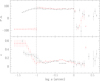 |
Fig. 3. Ellipticity and PA as a function of the semimajor axis in the F606W (red dots) and F814W (black dots) filters of ACS/HST for GC1 in M 81. Dashed lines indicate the points of 0.1 and 1.0 arcsec along the semimajor axis. |
Ellipticities and position angles of GC1 in M 81.
It is well known that raw output from the ELLIPSE package is in terms of counts s−1 pixel−1. So, we multiplied it by 400 = (1 px/0.05 arcsec)2 to convert to counts s−1 arcsec−2. In addition, we transformed the counts to surface brightness in magnitudes calibrated on the VEGAMAG system, using Eq. (4) (from the ACS Handbook)2,
 (4)
(4)
In this paper, we worked in terms of linear intensity instead of using surface brightness in magnitudes as previous authors have done (see Ma et al. 2017, and references therein), since occasional oversubtraction of the background during the multidrizzling in the automatic reduction pipeline leads to ‘negative’ counts in some pixels (see Barmby et al. 2007, for details). Finally, we transformed counts to surface brightness in intensity using Eq. (5),
 (5)
(5)
The zero-point conversion factors used in Eqs. (4) and (5) for each filter are from Table 2 of Wang & Ma (2013). The calibrated intensity profiles of GC1 obtained using Eq. (5) are listed in Table 4. Column 7 of Table 4 gives a flag for each point, which has the same meaning as defined by Barmby et al. (2007) and McLaughlin et al. (2008). The points flagged with ‘OK’ were used to constrain the model fit. The points flagged with ‘DEP’ lead to excessive weighting of the central regions of objects (see Ma et al. 2020, for details), and the points flagged with ‘BAD’ deviate strongly from their neighbors or show irregular features. The points flagged with ‘DEP’ and BAD were not used to constrain the model fit.
Intensity profiles for GC1 of M 81.
4.2. Point-spread function
Rhodes et al. (2006) pointed out that the point-spread function models are critical to accurately measure the shapes of objects in images taken with HST. In this paper, we chose not to deconvolve the data, instead fitting structural models after convolving them with a simple analytic description of the PSF as previous authors have done (see Ma et al. 2017, and references therein). Wang & Ma (2013) derived a simple analytic description of the PSFs for the ACS/WFC models (their Eq. (4)), which is used here.
5. Model fitting
5.1. Structural models
As was done by previous authors (see Ma et al. 2017, and references therein), we used three structural models to fit surface profiles of GC1 in M 81. These three models are given by King (1966), Wilson (1975), and Sérsic (1968) (hereafter the ‘King model’, ‘Wilson model’, and ‘Sérsic model’, respectively). McLaughlin et al. (2008) gave a detailed explanation for the three structural models, and we give a simple description of them here.
It is well known that the King model is most commonly used in studies of star clusters. And the King model that is used here is of a single-mass, isotropic, modified isothermal sphere, which was developed by Michie (1963) and King (1966). In fact, King (1962) found an empirical formula that represents the density from the centre to the edge in GCs, which is also called the King model. The Wilson model is presented by Wilson (1975), which is defined by an alternate modified isothermal sphere based on the ad hoc stellar distribution function of Wilson (1975). And the Wilson model has more extended envelope structures than the King model. The Sérsic model is also called the R1/n model, which is defined by directly parametrising the observable surface density profile. Tanvir et al. (2012) found that 60% of M31 classical GCs in their sample exhibit a cuspy core which are reasonably well fitted by the Sérsic model of index n ∼ 2 − 6.
5.2. Fits
We fitted the three structural models mentioned in Sect. 5.1 to the brightness profiles of GC1 in this section. This fitting first includes selecting a value for the scale radius r0 and computing the dimensionless model profile  . And then we convolved the models with PSFs for the filters used here to yield the product
  ,
,
![Mathematical equation: $$ \begin{aligned} \widetilde{I}_{\rm mod}^{*} (R | r_0) = \int \!\!\!\int _{-\infty }^{\infty } \widetilde{I}_{\rm mod}(R^\prime /r_0) \widetilde{I}_{\rm PSF} \left[(x-x^\prime ),({ y}-{ y}^\prime )\right]\mathrm{d}x^\prime \mathrm{d}{ y}^{\prime }, \end{aligned} $$](/articles/aa/full_html/2021/05/aa40574-21/aa40574-21-eq10.gif) (6)
(6)
where R2 = x2 + y2 and R′2 = x′2 + y′2. Furthermore,  is the PSF profile normalised to unit total luminosity, and it was computed using Eq. 4 from Wang & Ma (2013). We derived the best-fitting model by calculating and minimising χ2 as the sum of squared differences between model intensities and observed intensities with extinction corrected,
![Mathematical equation: $$ \begin{aligned} \chi ^2=\sum _{i}{\frac{[I_{\rm obs}(R_i)-I_0\widetilde{I}_{\rm mod}^{*}(R_i|r_0) -I_{\rm bkg}]^2}{\sigma _{i}^{2}}}. \end{aligned} $$](/articles/aa/full_html/2021/05/aa40574-21/aa40574-21-eq12.gif) (7)
(7)
In the fitting, we allowed for a non-zero background Ibkg. The uncertainties of observed intensities listed in Table 4 were used as weights.
We plotted the fitting for GC1 in M 81 in Fig. 4. The observed intensity profile is plotted as a function of the logarithmic projected radius. The open squares are the data points used in the model fitting, while the crosses are points flagged as DEP or BAD, which were not used to constrain the fit. Table 5 lists the basic and structural parameters of all model fits to GC1, with a simple description of each parameter and column at the end of Table 5. Error bars on all these parameters are defined in the same way as in McLaughlin et al. (2008).
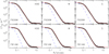 |
Fig. 4. Surface brightness profiles of and model fits to GC1, with the data of the F606W and F814W bands from top to bottom. The three panels in each line from left to right are the fits to the King model (K66), Wilson model (W), and Sérsic model (S). The open squares are the data points included in the model fitting, while the crosses are points flagged as DEP or BAD, which are not used to constrain the fit. The best fitting models are shown with a red solid line. The blue dashed lines represent the shapes of the PSFs for the filters used. |
Structural parameters of GC1 in M 81.
5.3. Comparison to previous results and discussion
Mayya et al. (2013) studied the structural parameters of GC1 using the HST images in the ACS/WFC F435W and F814W filters. In this paper, we studied the structural parameters of GC1 using the HST images in the ACS/WFC F606W and F814W filters. We fitted multiple models for the structural and dynamical parameters and chose the best fits. We found that the classic King model is not the best fit to its structural and dynamical parameters. And our fits estimate a very large tidal radius for this cluster, playing into the scientific question of the origins of GC1. The large tidal radius, its ellipticity, and its large half-light radius, which are obtained here, are in favour of GC1 being a former NSC. The data that challenge this hypothesis, mostly derived from the earlier studies, are GC1’s relatively high metallicity (see Sect. 3.1) (although this would not be inconsistent with a NSC in a relatively massive dwarf satellite), its short star formation history (Mayya et al. 2013), and its disk-like radial velocity (Nantais & Huchra 2010) combined with being projected onto the disk. A possible explanation for all of these points is that GC1 was at the nucleus of a relatively massive dwarf galaxy or protogalaxy that was accreted onto M 81 quite early in the galaxy’s formation history, stopping local gas flow into the cluster that would allow it to have a longer and more complex star formation history. However, more details of the star formation history and stellar population would likely require an even more detailed spectroscopic study of specific elemental abundances along the lines (Sakari et al. 2021), telescope time, and instrument capability permitting. Our results here may provide more insight as to the nature of this cluster and its implications for the role of accretion of dwarf satellites in the formation of M 81 and similar massive galaxies. The results of Mayya et al. (2013) show that the positions and ellipticities of GC1 in the two filters remain almost constant between 0.25 and 1 arcsec. Our results also present that the positions and ellipticities of GC1 in the ACS/WFC F606W and F814W filters remain almost constant between 0.1 and 1 arcsec. So, our results are in agreement with those of Mayya et al. (2013). In addition, Mayya et al. (2013) fitted the brightness profiles of GC1 with an empirical King model after convolving it with the PSF of the image in each of the ACS/WFC F435W and F814W filters. It is well known that an empirical King model includes three parameters which are needed to describe the structure of a cluster: a core radius rc, a tidal radius rt, and a richness factor log(rt/rc). Mayya et al. (2013) found that the empirical King model fits well the profile of GC1 from the centre to the edge in the F814W filter. However, Mayya et al. (2013) show that the empirical King model cannot fit the central profile of GC1 in the F435W filter well. Lastly, Mayya et al. (2013) obtained the core radius rc = 1.2 pc and the tidal radius rt = 93 pc in the F814W filter as typical values for GC1. In addition, Mayya et al. (2013) used the photometric data obtained by the ELLIPSE task to derive the half-light radius Reff of GC1. They only derived the Reff of GC1 in the F814W filter to be 5.6 pc. In this paper, we studied the structural parameters of GC1 using the HST images in the ACS/WFC F606W and F814W filters. We used three structural models to fit the brightness profiles of GC1 in M 81 based on a χ2 minimisation test. Our results show that the three models can fit the profile of GC1 from the centre to the edge in both filters well, although the Wilson model fits the profiles of GC1 in the F606W filter best. Different models gave many different results for some structural parameters. The Wilson model gave a tidal radius (rt) that is much larger than that given by the King model, and the Sérsic model gave a scale radius and a core radius that are much smaller than those given by the King and Wilson models. We obtained a core radius of  pc and a half-light radius of
  pc by fitting the King model in the F814W filter, which are in agreement with those obtained by Mayya et al. (2013), however, we obtained a tidal radius of
  pc which is much smaller than that obtained by Mayya et al. (2013). From our results, we know that the Wilson model fit the profiles of GC1 in the F606W filter best. So, we derived the structural parameters in the F606W filter by fitting the Wilson model as typical values for GC1 in this paper. Therefore, in this paper, we derived the central surface brightness to be
  mag arcsec−2, the core radius to be
  pc, the half-light radius to be
  pc, and the tidal radius to be
  pc.
pc.
Finally, we want to emphasise that Wilson and Sérsic models fit the bright profiles of GC1 better than the King model does. In the F606W band, the Wilson model fits the data of GC1 much better than the King and Sérsic models; however, in the F814W band, the Sérsic model fits the data of GC1 better than the King and Wilson models (The values of the χ2 index are 75.0, 64.84, and 52.52 for the King, Wilson, and Sérsic models, respectively.). In particular, in the F814W band, GC1 has an index of n > 2 derived from the Sérsic model fits, which implies a very strongly peaked central density profile. So we argue that GC1 may be a core-collapsed cluster. It is known that when a cluster is in a core-collapsed stage, the binaries at the centre of the cluster have provided a source of energy to halt the collapse. It is fortunate that the ROSAT and Chandra observations, which were presented by Immler & Wang (2001) and Swartz et al. (2003), have detected X-ray emissions from GC1 (see Mayya et al. 2013, for details). In addition, Mayya et al. (2013) calculated the expected tidal radius of GC1 to be 116 pc. The tidal radius  pc obtained here is much larger than the expected tidal radius. So, we argue that the dynamical evolution of GC1 is being affected by the tidal forces of the parent galaxy.
It is well known that the distribution of stellar systems in the luminosity versus half-light radius plane can give interesting information on their evolutionary history. van den Bergh & Mackey (2004) and Mackey & van den Bergh (2005) provided that in a plot of MV versus logRh, three objects (ω Centauri, M 54, and NGC 2419) in the Milky Way and G1 in M 31 are seen to fall well above the sharp upper envelope of the main distribution of the globular clusters, and Mackey & van den Bergh (2005) suggested that these four most luminous Local Group clusters are the cores of former dwarf galaxies. Figure 5 plots the half-light radius (Rh) versus absolute magnitude (MV) diagram, where data for GC1 are plotted along with those for the Galactic GCs from the online database of Harris (1996; 2010 update), for the extended star clusters (half-light radii greater than 5 pc) in NGC 4278, 4649, and 4697 from Forbes et al. (2013). In Fig. 5, we used the half-light radii of GC1 obtained by fitting the radial surface brightness profiles in the F606W band by the Wilson model, and the absolute magnitude (MV) was obtained using mV = 16.70 ± 0.023 obtained in Sect. 3.4. Figure 5 makes it evident that GC1 occupies the same area as extended star clusters. Therefore, we suggest that GC1 is more likely an accreted former NSC than a classical GC similar to most of those in the Milky Way.
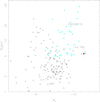 |
Fig. 5. Half-light radii (Rh) versus absolute magnitudes (MV) for GC1 in M 81 (filled red circle with error bar) in comparison with Galactic GCs from the online database of Harris (1996; 2010 update) GCs (cross). The filled cyan circles are the extended star clusters (half-light radii greater than 5 pc) in NGC 4278, 4649, and 4697 from Forbes et al. (2013). |
6. Summary
In this paper, we study one of the most massive GCs in the Local Group: GC1 in M 81. We largely reproduce previous results despite the smaller wavelength range, confirming that this cluster is indeed very old and massive, and it has an extended half-light radius similar to other very massive GCs.
(1) We derived the magnitudes in intermediate-band filters of the BATC system for GC1.
(2) We determined this cluster’s age and mass by comparing its SEDs (from 4000 to 20 000 Å, comprising photometric data in the 14 BATC intermediate-band and 2MASS near-infrared JHKs filters) with theoretical stellar population synthesis models.
(3) The age of GC1 obtained in this paper is 13.25 ± 2.80 Gyr, which shows that it is an old GC in M 81.
(4) The mass of GC1 obtained here is 1.19 − 1.66 × 10⁷M⊙, which shows that it is one of the most massive clusters in the nearby Universe.
(5) We derived the structural parameters of GC1 based on the HST images from fitting its surface brightness profiles to three different models. We found that the classic King model is not the best fit to its structural and dynamical parameters, and our fits estimate a very large tidal radius for this cluster, implying a dynamical influence from M 81.
(6) The Rh versus MV diagram shows that GC1 occupies the same area of the extended star clusters. So, we suggest that GC1 is more likely a former NSC from an accreted dwarf satellite than a classical GC similar to most of those in the Milky Way.
These conclusions are a valuable reference for further study of GC1 in the future. Also, the photometric part in this paper is less novel, but it confirms the previous results in a more restricted wavelength range, which has useful implications for making future studies easier.
Acknowledgments
We are deeply indebted to the referee for providing rapid and thoughtful report that helped improve the original manuscript greatly. This study has been supported by National Key R&D Program of China No. 2019YFA0405501 and by the National Natural Science Foundation of China (NSFC, No. 11873053).
References
- Anders, P., & Fritze-v Alvensleben, U. 2003, A&A, 401, 1063 [NASA ADS] [CrossRef] [EDP Sciences] [Google Scholar]
- Antonini, F., Barausse, E., & Silk, J. 2015, ApJ, 812, 72 [NASA ADS] [CrossRef] [Google Scholar]
- Ashman, K. M., & Zepf, S. E. 1992, ApJ, 384, 50 [NASA ADS] [CrossRef] [Google Scholar]
- Barmby, P., Holland, S., & Huchra, J. 2002, AJ, 123, 1937 [NASA ADS] [CrossRef] [Google Scholar]
- Barmby, P., McLaughlin, D. E., Harris, W. E., Harris, G. L. H., & Forbes, D. A. 2007, AJ, 133, 2764 [Google Scholar]
- Barmby, P., Perina, S., Bellazzini, M., et al. 2009, AJ, 138, 1667 [NASA ADS] [CrossRef] [Google Scholar]
- Beasley, M. A., Baugh, C. M., Forbes, D. A., Sharples, R. M., & Frenk, C. S. 2002, MNRAS, 333, 383 [NASA ADS] [CrossRef] [MathSciNet] [Google Scholar]
- Bessell, M. S., & Brett, J. M. 1988, PASP, 100, 1134 [NASA ADS] [CrossRef] [Google Scholar]
- Brodie, J. P., & Strader, J. 2006, ARA&A, 44, 193 [NASA ADS] [CrossRef] [Google Scholar]
- Cardelli, J. A., Clayton, G. C., & Mathis, J. S. 1989, ApJ, 345, 245 [NASA ADS] [CrossRef] [Google Scholar]
- Carpenter, J. M. 2001, AJ, 121, 2851 [NASA ADS] [CrossRef] [Google Scholar]
- Chandar, R., Ford, H. C., & Tsvetanov, Z. 2001, AJ, 122, 1330 [NASA ADS] [CrossRef] [Google Scholar]
- Côté, P., Marzke, R. O., & West, M. J. 1998, ApJ, 501, 554 [NASA ADS] [CrossRef] [Google Scholar]
- Durrell, P. R., Sarajedini, A., & Chandar, R. 2010, ApJ, 718, 1118 [NASA ADS] [CrossRef] [Google Scholar]
- Fan, X., Burstein, D., Chen, J.-S., et al. 1996, AJ, 112, 628 [NASA ADS] [CrossRef] [Google Scholar]
- Forbes, D. A., Brodie, J. P., & Grillmair, C. J. 1997, AJ, 113, 1652 [NASA ADS] [CrossRef] [Google Scholar]
- Forbes, D. A., Pota, V., Usher, C., et al. 2013, MNRAS, 435, L6 [NASA ADS] [CrossRef] [Google Scholar]
- Forbes, D. A., Bastian, N., Gieles, M., et al. 2018, Proc. R. Soc. A, 474, 20170616 [Google Scholar]
- Freedman, W. L., Wilson, C. D., & Madore, B. F. 1994, ApJ, 427, 628 [NASA ADS] [CrossRef] [Google Scholar]
- Girardi, L., Castelli, F., Bertelli, G., & Nasi, E. 2007, A&A, 468, 657 [NASA ADS] [CrossRef] [EDP Sciences] [Google Scholar]
- Hanes, D. A. 1977a, MNRAS, 179, 331 [Google Scholar]
- Hanes, D. A. 1977b, MNRAS, 180, 309 [NASA ADS] [CrossRef] [Google Scholar]
- Harris, W. E. 1991, ARA&A, 29, 543 [NASA ADS] [CrossRef] [Google Scholar]
- Harris, W. E. 1996, AJ, 112, 1487 [NASA ADS] [CrossRef] [Google Scholar]
- Immler, S., & Wang, Q.-D. 2001, ApJ, 554, 202 [NASA ADS] [CrossRef] [Google Scholar]
- Jang, I.-S., Lim, S., Park, H. S., & Lee, M. G. 2012, ApJ, 751, L19 [Google Scholar]
- Jenkner, H., Lasker, B. M., Sturch, C. R., et al. 1990, AJ, 99, 2082 [Google Scholar]
- Johnson, C. I., Dupree, A. K., Mateo, M., et al. 2020, AJ, 159, 254 [CrossRef] [Google Scholar]
- Kaviraj, S., Rey, S. C., Rich, R. M., Yoon, S. J., & Yi, S. K. 2007, MNRAS, 381, L74 [NASA ADS] [CrossRef] [Google Scholar]
- King, I. R. 1962, AJ, 67, 471 [NASA ADS] [CrossRef] [Google Scholar]
- King, I. R. 1966, AJ, 71, 64 [Google Scholar]
- Kong, X., Zhou, X., Chen, J., et al. 2000, AJ, 119, 2745 [NASA ADS] [CrossRef] [Google Scholar]
- Kruijssen, J. M. D. 2015, MNRAS, 454, 1658 [NASA ADS] [CrossRef] [Google Scholar]
- Kurth, O. M., Fritze-v Alvensleben, U., & Fricke, K. J. 1999, A&AS, 139, 19 [Google Scholar]
- Landolt, A. U. 1983, AJ, 88, 439 [NASA ADS] [CrossRef] [Google Scholar]
- Li, H., & Gnedin, O. Y. 2014, ApJ, 796, 10 [NASA ADS] [CrossRef] [Google Scholar]
- Ma, J. 2015, AJ, 149, 15 [NASA ADS] [CrossRef] [Google Scholar]
- Ma, J., de Grijs, R., Yang, Y., Zhou, X., Chen, J., Jiang, Z., Wu, Z., & Wu, J. 2006, MNRAS, 368, 1443 [NASA ADS] [CrossRef] [Google Scholar]
- Ma, J., de Grijs, R., Fan, Z., et al. 2009, Res. Astron. Astrophys., 9, 641 [Google Scholar]
- Ma, J., Wang, S., Wu, Z., et al. 2012, AJ, 143, 29 [NASA ADS] [CrossRef] [Google Scholar]
- Ma, J., Wang, S., Wu, Z., et al. 2017, MNRAS, 468, 4513 [NASA ADS] [CrossRef] [Google Scholar]
- Ma, J., Wang, S., Wang, S., et al. 2020, MNRAS, 496, 374 [Google Scholar]
- Mackey, A., & van den Bergh, S. 2005, MNRAS, 360, 631 [NASA ADS] [CrossRef] [Google Scholar]
- Martini, P., & Ho, L.-C. 2004, ApJ, 610, 233 [Google Scholar]
- Mayya, Y., Rosa-González, D., Santiago-Cortés, M., et al. 2013, MNRAS, 436, 2763 [Google Scholar]
- McLaughlin, D. E., & van der Marel, R. P. 2005, ApJS, 161, 304 [NASA ADS] [CrossRef] [Google Scholar]
- McLaughlin, D. E., Barmby, P., Harris, W. E., Forbes, D. A., & Harris, G. L. H. 2008, MNRAS, 384, 563 [Google Scholar]
- Meylan, G. 2002, in Extragalactic Star Clusters, eds. D. Geisler, E. K. Grevel, & D. Minniti (San Francisco: ASP), IAUS, Symp.207, 555 [Google Scholar]
- Meylan, G., Sarajedini, A., Jablonka, P., Djorgovski, S., Bridges, T., & Rich, R. 2001, AJ, 122, 830 [NASA ADS] [CrossRef] [Google Scholar]
- Michie, R. W. 1963, MNRAS, 125, 127 [NASA ADS] [CrossRef] [Google Scholar]
- Nantais, J. B., & Huchra, J. P. 2010, AJ, 139, 2620 [NASA ADS] [CrossRef] [Google Scholar]
- Nantais, J. B., Huchra, J. P., McLeod, B., Strader, J., & Brodie, J. P. 2010, AJ, 139, 1413 [Google Scholar]
- Neumayer, N., Seth, A., & Böker, T. 2020, A&ARv, 28, 4 [CrossRef] [Google Scholar]
- Oke, J. B., & Gunn, J. E. 1983, ApJ, 266, 713 [NASA ADS] [CrossRef] [Google Scholar]
- Perelmuter, J. M., & Racine, R. 1995, AJ, 109, 1055 [NASA ADS] [CrossRef] [Google Scholar]
- Pfeffer, J., Kruijssen, J. M. D., Crain, R. A., & Bastian, N. 2018, MNRAS, 475, 4309 [NASA ADS] [CrossRef] [Google Scholar]
- Rhodes, J. D., Massey, R., Albert, J., et al. 2006, in The 2005 HST Calibration Workshop: Hubble After the Transition to Two-Gyro Mode, eds. A. M.Koekemoer, P.Goudfrooij, & L. L.Dressel, 21 [Google Scholar]
- Sakari, C. M., Shetrone, M. D., McWilliam, A., & Wallerstein, G. 2021, MNRAS, 502, 5745 [Google Scholar]
- Salpeter, E. E. 1955, ApJ, 121, 161 [Google Scholar]
- Santiago-Cortés, M., Mayya, Y. D., & Rosa-González, D. 2010, MNRAS, 405, 1293 [Google Scholar]
- Schroder, L. L., Brodie, J. P., Kissler-Patig, M., Huchra, J. P., & Phillips, A. C. 2002, AJ, 123, 2473 [NASA ADS] [CrossRef] [Google Scholar]
- Schulz, J., Fritze-v Alvensleben, U., Möller, C. S., & Fricke, K. J. 2002, A&A, 392, 1 [NASA ADS] [CrossRef] [EDP Sciences] [Google Scholar]
- Sérsic, J. L. 1968, Atlas de Galaxias Australes (Cordoba: Obs. Astronomico) [Google Scholar]
- Stetson, P. B. 1987, PASP, 99, 191 [Google Scholar]
- Swartz, D. A., Ghosh, K. K., McCollough, M. L., et~al. 2003, ApJS, 144, 213 [NASA ADS] [CrossRef] [Google Scholar]
- Tanvir, N. R., Mackey, A. D., Ferguson, A. M. N., et al. 2012, MNRAS, 422, 162 [NASA ADS] [CrossRef] [Google Scholar]
- Taylor, M. A., Puzia, T. H., Harris, G. L., Harris, W. E., Kissler-Patig, M., & Hilker, M. 2010, ApJ, 712, 1191 [NASA ADS] [CrossRef] [Google Scholar]
- van den Bergh, S., & Mackey, A. D. 2004, MNRAS, 354, 713 [NASA ADS] [CrossRef] [Google Scholar]
- Villanova, S., Geisler, D., Gratton, R. G., & Cassisi, S. 2014, ApJ, 791, 107 [Google Scholar]
- Wang, S., & Ma, J. 2013, AJ, 146, 20 [Google Scholar]
- West, M. J., Côté, P., Marzke, R. O., & Jordán, A. 2004, Nature, 427, 31 [Google Scholar]
- Wilson, C. P. 1975, AJ, 80, 175 [NASA ADS] [CrossRef] [Google Scholar]
- Yan, H. J., Burstein, D., Fan, X., et al. 2000, PASP, 112, 691 [NASA ADS] [CrossRef] [Google Scholar]
- Zheng, Z., Shang, Z., Su, H., et al. 1999, AJ, 117, 2757 [NASA ADS] [CrossRef] [Google Scholar]
- Zhou, X., Jiang, Z.-J., Xue, S.-J., et al. 2001, Chin. J. Astron. Astrophys., 1, 372 [Google Scholar]
- Zhou, X., Jiang, Z., Ma, J., et al. 2003, A&A, 397, 361 [NASA ADS] [CrossRef] [EDP Sciences] [Google Scholar]
- Zinnecker, H., Keable, C. J., Dunlop, J. S., Cannon, R. D., & Griffiths, W. K. 1988, in The Harlow-Shapley Symposium on Globular Cluster Systems in Galaxies (Dordrecht: Kluwer), Proc. IAU Symp., 126, 603 [NASA ADS] [CrossRef] [Google Scholar]
All Tables
All Figures
|
Fig. 1. Left panel: image of GC1 in the BATC g band obtained with the 60/90 cm Schmidt telescope in the BATC Multicolour Sky Survey, of which the circle is photometric aperture adopted in this paper. Right panel: image of GC1 observed in the F606W filter of ACS/HST, of which the circle around GC1 is of a 6 arcsec radius. |
| In the text | |
|
Fig. 2. Best-fitting, integrated theoretical GALEV SEDs compared to the intrinsic SEDs of GC1. The photometric measurements are shown as symbols with error bars (vertical error bars for photometric uncertainties and horizontal ones for the approximate wavelength coverage of each filter). The open circles represent the calculated magnitudes of the model SED for each filter. |
| In the text | |
|
Fig. 3. Ellipticity and PA as a function of the semimajor axis in the F606W (red dots) and F814W (black dots) filters of ACS/HST for GC1 in M 81. Dashed lines indicate the points of 0.1 and 1.0 arcsec along the semimajor axis. |
| In the text | |
|
Fig. 4. Surface brightness profiles of and model fits to GC1, with the data of the F606W and F814W bands from top to bottom. The three panels in each line from left to right are the fits to the King model (K66), Wilson model (W), and Sérsic model (S). The open squares are the data points included in the model fitting, while the crosses are points flagged as DEP or BAD, which are not used to constrain the fit. The best fitting models are shown with a red solid line. The blue dashed lines represent the shapes of the PSFs for the filters used. |
| In the text | |
|
Fig. 5. Half-light radii (Rh) versus absolute magnitudes (MV) for GC1 in M 81 (filled red circle with error bar) in comparison with Galactic GCs from the online database of Harris (1996; 2010 update) GCs (cross). The filled cyan circles are the extended star clusters (half-light radii greater than 5 pc) in NGC 4278, 4649, and 4697 from Forbes et al. (2013). |
| In the text | |
Current usage metrics show cumulative count of Article Views (full-text article views including HTML views, PDF and ePub downloads, according to the available data) and Abstracts Views on Vision4Press platform.
Data correspond to usage on the plateform after 2015. The current usage metrics is available 48-96 hours after online publication and is updated daily on week days.
Initial download of the metrics may take a while.