| Issue |
A&A
Volume 649, May 2021
|
|
|---|---|---|
| Article Number | A20 | |
| Number of page(s) | 7 | |
| Section | Cosmology (including clusters of galaxies) | |
| DOI | https://doi.org/10.1051/0004-6361/202039936 | |
| Published online | 03 May 2021 | |
BAO angular scale at zeff = 0.11 with the SDSS blue galaxies
1
Centro de Estudos Superiores de Tabatinga, Universidade do Estado do Amazonas, 69640-000 Tabatinga, AM, Brazil
e-mail: This email address is being protected from spambots. You need JavaScript enabled to view it.
2
Observatório Nacional, Rua General José Cristino 77, São Cristóvão, 20921-400 Rio de Janeiro, RJ, Brazil
3
Instituto Nacional de Pesquisas Espaciais, Av. dos Astronautas 1758, Jardim da Granja, São José dos Campos, SP, Brazil
Received:
18
November
2020
Accepted:
18
March
2021
Abstract
Aims. We measure the transverse baryon acoustic oscillations (BAO) signal in the local Universe using a sample of blue galaxies from the Sloan Digital Sky Survey (SDSS) survey as a cosmological tracer.
Methods. The method is weakly dependent on a cosmological model and is suitable for 2D analyses in thin redshift bins to investigate the SDSS data in the interval z ∈ [0.105, 0.115].
Results. We detect the transverse BAO signal θBAO = 19.8°±1.05° at zeff = 0.11, with a statistical significance of 2.2σ. Additionally, we perform tests that confirm the robustness of this angular BAO signature. Supported by a large set of log-normal simulations, our error analyses include statistical and systematic contributions. In addition, considering the sound horizon scale calculated by the Planck Collaboration, rsPlanck, and the θBAO value obtained here, we obtain a measurement of the angular diameter distance DA(0.11) =258.31 ± 13.71 h−1 Mpc. Moreover, combining this θBAO measurement at low redshift with other BAO angular scale data reported in the literature, we perform statistical analyses for the cosmological parameters of some Lambda cold dark matter type models.
Key words: cosmological parameters / large-scale structure of Universe / cosmology: observations
© ESO 2021
1. Introduction
Embedded in the 3D distribution of cosmic luminous matter are geometrical signatures from the primordial baryon acoustic oscillations (BAO; Peebles & Yu 1970; Sunyaev & Zeldovich 1970; Bond & Efstathiou 1987; Eisenstein et al. 2005; Cole et al. 2005). They can be statistically revealed in large-scale and numerically dense astronomical surveys and are used as a standard ruler to measure our distance to the data region. These analyses are performed by studying different cosmological tracers from a variety of astronomical surveys, such as the Sloan Digital Sky Survey (SDSS), the 6dF Galaxy Survey, and the WiggleZ Dark Energy Survey (Alam et al. 2017, 2020; Beutler et al. 2011; Blake et al. 2011). A set of precise distance measurements for several redshift values will unambiguously describe the dynamics of the universe (Eisenstein & Hu 1998; Bassett & Hlozek 2010; Eisenstein et al. 2007).
The BAO distance measurements are obtained using two-point statistics in at least two ways. The first approach, based on the 3D information, assumes a fiducial cosmology to transform the redshift of each cosmic object into its radial distance, and with the two angular coordinates measured in the survey, the comoving distance between all possible pairs is calculated to construct the two-point correlation function (2PCF). The BAO signal obtained with this approach determines the sound horizon scale at the end of the baryon drag epoch, rs, and the spherically averaged distance DV (Beutler et al. 2011; Blake et al. 2011; Alam et al. 2017; Abbott et al. 2019). The second approach uses 2-dimensional (2D) information: the data in a redshift shell are projected on the celestial sphere. With the two angular coordinates of each cosmic object, the angular separation between pairs is then calculated and the two-point angular correlation function (2PACF) is calculated, where the BAO angular scale provides a measure of the angular diameter distance DA if rs is known. To minimize projection effects that would affect this measurement, the data should be in a thin redshift shell (Sánchez et al. 2011; Carnero et al. 2012; Carvalho et al. 2016).
In addition to the advantages and disadvantages of each approach, the 2D method is a quasi model-independent procedure, with a weak dependence on the fiducial cosmology that we explained below. We adopt it here to measure the BAO angular scale θBAO. The 2D approach was not widely applied to early data releases because the number density of cosmic objects was not high enough to provide a good BAO signal-to-noise ratio (S/N) in thin redshift shells. However, the current data releases have suitably increased this quantity. Several studies reported 2D BAO measurements using luminous red galaxies (LRG) and quasar samples at several redshifts (Sánchez et al. 2011; Carnero et al. 2012; Salazar-Albornoz et al. 2017; Carvalho et al. 2016; Abbott et al. 2019; de Carvalho et al. 2018). The present work extends these analyses with a 2D BAO measurement at low redshift, zeff = 0.11 from an unusual cosmological tracer, the SDSS sample of blue galaxies (York et al. 2000; Avila et al. 2019).
This work is organized as follows. Section 2 provides the details of the blue galaxy sample selection from the SDSS data set, the generation of the random catalog, and the simulations we used. Section 3 describes the statistical tools employed in the 2D clustering analyses. In Sect. 4 we describe our main results, giving details on the 2D analyses and our estimate of the BAO angular scale, while in Sect. 5 we present the discussion of our results and final conclusions.
2. Data description
2.1. Blue galaxy sample and random catalogs
We used the sample of blue star-forming galaxies analyzed in Avila et al. (2019). The selected data are part of the twelfth public data release, DR12, of the SDSS collaboration (Alam et al. 2015). We considered the low-redshift SDSS blue galaxies displayed in the north galactic cap with the footprint observed in Fig. 1, covering an area of ∼7000 deg2.
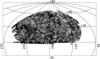 |
Fig. 1. Sample of SDSS blue galaxies in equatorial coordinates J2000 (in degrees). |
To optimize between sample variance and shot noise, the galaxy field has to be weighted. To do this, we assigned weights to each galaxy based on the average local density in the analyzed region by using the Feldman-Kaiser-Peacock (FKP) weights (Feldman et al. 1994). This is a scale-independent weighting that depends on redshift, wFKP(z) = 1/(1+n(z)P0), where P0 is the amplitude of the power spectrum and n(z) is the number density of galaxies. We used P0 ≃ 10 000 h−3 Mpc3, the power amplitude relevant to the BAO signal k ≈ 0.15 h Mpc−1 (Eisenstein et al. 2005; Beutler et al. 2011; Carter et al. 2018). Therefore the effective redshift of our sample, zeff, calculated with the FKP galaxy weights, wi ≡ w(zi) = wFKP(zi), is obtained through (see, e.g., Carter et al. 2018)
 (1)
(1)
where Ng is the total number of galaxies in the sample.
We searched for a statistically significant angular BAO detection at the lowest redshift. After analyzing bins with a large number of galaxies (to minimize the statistical noise) that are located in a thin redshift bin (to minimize the nonlinear contributions due to the projection effect, see, e.g., Sánchez et al. 2011), we selected the data sample contained in the thin redshift bin 0.105 ≤ z ≤ 0.115, with δz = 0.01 and zeff = 0.11. This bin contains Ng = 15 942 blue galaxies.
We would like to point out that the comoving volume survey containing these Ng = 15 942 blue galaxies is V ≃ 0.0063 (Gpc/h)3. This seems to be a small volume in which to look for a transverse BAO signal, but the important parameter for these analyses is the number density n. For this sample of blue galaxies, the number density is n = Ng/V ≃ 2.5 × 10⁶(h/Gpc)3. For comparison, nLRG = 104 − 105 (h/Gpc)3 for the SDSS LRG sample analyzed in the 3D BAO detection (Eisenstein et al. 2005), or nquasars ≃ 7.3 × 10³ (h/Gpc)3 for the 2D BAO detection using a sample of SDSS quasars (de Carvalho et al. 2018).
The random catalogs are an important ingredient in our analyses. They are necessary to extract the BAO features from the data. For this, they must have properties in common to those observed in the SDSS blue galaxy catalog. We produced 50 random catalogs for the 2D analyses (with Nsim ≃ 16 000 in each catalog) with Poisson-distributed objects (Peebles & Hauser 1974) sharing the observational features of the data set in analyses (i.e., the same number density and footprint sky area as the SDSS data). Our set of random catalogs was produced following the method described in the Appendix B of de Carvalho et al. (2018), where they were satisfactorily tested through a null test analysis (see, e.g., Sect. 5 of Landy & Szalay 1993) to confirm that they do not introduce spurious signals.
2.2. Log-normal simulations
To estimate the error bars of the 2PACF and the statistical significance of our results, we used the covariance matrix built from full-sky log-normal simulations that we produced with the FLASK code1 (Xavier et al. 2016; de Carvalho et al. 2020). We generated a set of 1000 simulations for which we assume the Lambda cold dark matter (ΛCDM) cosmological parameters measured by the Planck Collaboration VI (2020), including all effects available such as lensing, redshift space distortions (RSD), and nonlinear clustering to compute with the code CAMBsources2 (Challinor & Lewis 2011) the fiducial angular power spectrum Cℓ that was used as input.
This set of simulations was designed to be used in the angular analyses where we assumed a top-hat redshift bin (0.105 ≤ z ≤ 0.115) with a surface number density of 2.3 galaxies per deg2 (the same as in SDSS data). These simulated data share the observational features of the data set in the analyses, that is, the same number density and footprint sky area, and they were also weighted by the FKP scheme. The number of simulated cosmic objects in each catalog is Nsim ≃ 16 000. For this set of simulated maps, we adopted an angular resolution of 0.11 deg2, given by the HEALPix3 (Górski et al. 2005) parameter Nside = 512.
3. Two-point correlation estimator
We performed a 2D BAO measurement at low redshift with the SDSS blue galaxy sample. This measurement complements similar 2D analyses performed following the same method applied to other cosmological tracers, such as LRG and quasars, at several redshifts (Carvalho et al. 2016, 2020; Alcaniz et al. 2017; de Carvalho et al. 2018). The 2D BAO studies were performed by applying the 2PACF to the thin redshift bin 0.105 ≤ z ≤ 0.115. Additionally, supported by a large set of log-normal simulations, we describe how the covariance matrix was used in the error analyses, including statistical and systematic contributions.
3.1. Two-point angular correlation function
In the 2D analysis, the 2PACF (Peebles & Yu 1970; Landy & Szalay 1993) estimates the angular correlation for data pairs projected on the celestial sphere (for alternative clustering analyses, see, e.g., Avila et al. 2018, 2019; Bengaly et al. 2017; Feldbrugge et al. 2019; Novaes et al. 2016, 2018; Marques & Bernui 2020; Marques et al. 2020; Pandey & Sarkar 2020; Sosa Nuñez & Niz 2020). Considering blue galaxies in a redshift shell, the 2PACF measures the angular diameter distance DA due to the transverse BAO signal of the sound horizon scale there, where this signature appears as a bump at certain angular scale. The expression for the 2PACF estimator, ω(θ), is given by
 (2)
(2)
with θ the angular separation between any pair of blue galaxies A, B, given by
![Mathematical equation: $$ \begin{aligned} \theta =\arccos [\sin {\delta _{A}}\sin {\delta _{B}}+ \cos {\delta _{A}}\cos {\delta _{B}}\cos (\alpha _{A}-\alpha _{B})] , \nonumber \end{aligned} $$](/articles/aa/full_html/2021/05/aa39936-20/aa39936-20-eq4.gif)
where αA, αB and δA, δB are the right ascension and declination coordinates of the blue galaxies A and B, respectively (Landy & Szalay 1993; Sánchez et al. 2011).
To find the angular scale θFIT of the BAO bump in the 2PACF, ω(θ), we used the method proposed by Sánchez et al. (2011), which is based on the empirical parameterization of ω = ω(θ),
 (3)
(3)
where A, B, γ, C, θFIT, and σFIT are free parameters. Therefore this equation provides the BAO bump best-fit, θFIT, and the width of the bump is σFIT.
The final measurement of the acoustic peak was obtained after accounting for the shift due to the projection effect (Sánchez et al. 2011; Carnero et al. 2012; Carvalho et al. 2016). In the 2D analyses, all galaxies in the redshift bin in the study with thickness δz are assumed to be projected onto the celestial sphere. Thus, the finite thickness of the shell, δz ≠ 0, produces a shift of the BAO peak. This shift is estimated through numerical analysis by assuming a fiducial cosmology (as we show in Sect. 4.2), but the results show that for thin shells, the shift is small and weakly dependent on the cosmological parameters (for details, see, e.g., Sánchez et al. 2011; Carvalho et al. 2016). The redshift shell should be as thin as possible to minimize the projection effect that affects the measurement by erasing the acoustic signature, but at the same time, it should be a numerically dense data set, enough to obtain a good BAO S/N. We calculate the shift to be applied to θFIT due the projection effect in Sect. 4.2.
3.2. Covariance matrix estimation
To estimate the covariance matrix and the significance of our results, we used the galaxy mocks described above (see Sect. 2.2). For each mock, we extracted the 2PACF information from a set of Nb bins in which the interval of θ values was divided. The covariance matrix for ω(θ) was estimated using the expression
![Mathematical equation: $$ \begin{aligned} \mathrm{Cov}_{ij} = \frac{1}{N}\sum _{k=1}^{N} \Big [{ w}_k(\theta _i)-\overline{{ w}}(\theta _i)\Big ] \Big [{ w}_k(\theta _j)-\overline{{ w}}(\theta _j)\Big ], \end{aligned} $$](/articles/aa/full_html/2021/05/aa39936-20/aa39936-20-eq6.gif) (4)
(4)
where the i and j indices represent each θ bin, i, j = 1, …, Nb, and wk is the 2PACF for the k-th mock catalog, with k = 1, …, N;  is the mean value for this statistics over the N = 1000 mocks in that bin. Finally, the error of w(θi) is the square root of the main diagonal,
  .
.
4. Clustering analyses in 2D
We studied the clustering of the SDSS blue galaxy sample performing 2D analysis. Using the estimator given by Eq. (2), ω(θ), we calculated the 2PACF for our sample of Ng = 15 942 galaxies in the redshift interval z ∈ [0.105, 0.115], with effective redshift zeff = 0.11. The 2PACF was calculated using TREECORR (Jarvis et al. 2004) for equally spaced values of θ in the interval 5° ≤θ ≤ 30°, in a total of Nb = 20 bins, which means that the bin size was 1.25°. To extract the BAO bump position, we used Eq. (3) to fit the 2PACF data through a least-squares method; the errors in the parameters correspond to the statistical uncertainties provided by the fitting procedure (the estimated covariance matrix of the parameters). The result is shown in Fig. 2, where θFIT = 19.42°. Our result for this procedure is summarized in Table 1, where we display the best-fit parameters obtained in this fitting approach using Eq. (3).
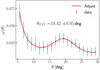 |
Fig. 2. BAO signature obtained in the 2PACF by analyzing the sample in the redshift interval z ∈ [0.105, 0.115], with δz = 0.01. The bin size in this 2PACF is 1.25°, and we use 50 random catalogs with the same observational features as the galaxy catalog. |
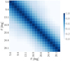 |
Fig. 3. Covariance matrix for the 2PACF obtained from Eq. (4) using the set of log-normal simulated maps (see Sect. 2.2). |
4.1. Statistical significance
The statistical significance of the BAO angular measurement was obtained through the χ2 method,
![Mathematical equation: $$ \begin{aligned} \chi ^2(\alpha ) = \left[{ w} - { w}^{fit }(\alpha )\right]^{T}\mathrm{Cov}^{-1} \left[{ w} - { w}^{fit }(\alpha )\right] , \end{aligned} $$](/articles/aa/full_html/2021/05/aa39936-20/aa39936-20-eq9.gif) (5)
(5)
where we used the inverse of the covariance matrix, Cov, estimated as described in Sect. 3.2 and shown in Fig. 3. The symbols [ ] and [ ]T represent column vectors and row vectors, respectively.
Following de Carvalho et al. (2018), we adjusted the parameters of Eq. (3) based on the minimum χ2 method for α ∈ [0.85, 1.25], which is called the scale dilation parameter, for two cases: considering C as free parameter, C ≠ 0 ( ), and imposing C = 0 (
 ), where
  corresponds to αmin = 0.996, the latter case representing the non-BAO case. Table 1 shows the best-fit parameters obtained considering α = 1.
As a result, the best-fit4 of the non-BAO case (16 degrees of freedom, d.o.f.), compared to the BAO case (13 d.o.f.), is disfavored by Δχ2 = 8.93. Therefore our BAO angular detection has a statistical significance of 2.2σ, which is compatible with the distance of the C parameter from zero.
4.2. Projection effect in the 2PACF
To know the angular scale θBAO, we need to correct the θFIT due to the projection effect, which produces a shift in the BAO bump position (Sánchez et al. 2011). To quantify this shift, we first computed the expected angular BAO scale,  , corresponding to the bump position for the case δz = 0 calculated from the expected 2PACF,
 (6)
(6)
where z = zeff = (z1 + z2)/2, with z2 = z1 + δz, and ϕ(zi) is the normalized galaxy selection function at redshift zi. The function ξE is the 2PCF expected in the fiducial cosmology, given by (see, e.g., Sánchez et al. 2011)
 (7)
(7)
where j0 is the zeroth-order Bessel function, Pm(k, z) is the matter power spectrum, and b is the bias factor.
It is suitable to examine the RSD effect on the measurement of the angular BAO signature. For this we performed analyses that included the linear RSD by changing Pm(k, z) by (1 + β μ2)2Pm(k, z) in the Eq. (7), where we considered two cases: the linear,  , and the nonlinear,
  , matter power spectra produced using the numerical code CAMB (Challinor & Lewis 2011), at z = 0.11. We assumed the ΛCDM model with the cosmological parameters measured by the Planck Collaboration VI (2020). The term (1 + β μ2)2 corresponds to the Kaiser model for large-scale RSD (Kaiser 1987), where β, the velocity scale parameter is β = f/b, b is the linear bias, and f is the growth rate of cosmic structures, with f ≃ Ωm(z)0.55, where μ is the cosine of the angle between the wave vector k and the line of sight.
Our results show that the relative difference in the bump position between the linear matter power spectra with and without the linear RSD is 0.84%. For the nonlinear matter power spectra with and without the linear RSD, the relative difference in the bump position is equal to 0.70%. On the other hand, comparing the linear and the nonlinear matter power spectra cases, the differences in the bump position are 0.14% and 0.00% for the cases with and without the linear RSD effect, respectively. In all cases the relative differences are smaller than 1%, therefore we conclude that these effects on our angular BAO measurement are small and are included in the final error.
Next, we applied this procedure to our data, where δz = 0.01 is the thickness of the redshift bin used here, to find  . Then, the BAO angular scale, θBAO, is
 (8)
(8)
where  shifts the fitted value θFIT(z) to the correct acoustic scale θBAO(z), at z = zeff = 0.11.
Assuming the ΛCDM model with the cosmological parameters measured by Planck Collaboration VI (2020), we estimate  and
and  , which corresponds to Δθ = 1.96%. Consequently, θBAO(zeff = 0.11) = 19.8°. As shown by Sánchez et al. (2011), the choice of the fiducial cosmological model introduces a systematic error of 1% in the final θBAO error.
4.3. Robustness of the BAO signal
We performed a robustness test in the two-point angular correlation statistics to confirm the BAO signature in the 2PACF. To verify that the BAO signature corresponds to a robust detection, we performed the small-shifts criterion test (Carvalho et al. 2016; de Carvalho et al. 2018). The main idea here is to distinguish between the true BAO bump, which is expected to be smoothed, but survives, under weak perturbations in the galaxy positions, while other local maxima that originate in systematic effects or statistical noise tend to disappear in a reanalysis after the perturbations. For this, we first generated 100 modified galaxy catalogs by drawing the modified position of each galaxy resulting from a random Gaussian distribution with the mean equal to the original position and standard deviation σs, and for each modified catalog we calculated the 2PACF curve. The final 2PACF was estimated as the average over the 100 curves resulting from each of the modified galaxy catalogs, perturbed considering the standard deviation σs. We performed this process for the cases with σs = 1.0° ,2.0°, and 3.0°. In the calculation of each 2PACF we used the same set of 50 random catalogs as in the main analysis, always applying Eq. (2).
Our results are shown in Fig. 4, where we present the original data as black dots together with the three cases for σs that are printed as solid colored curves. As observed, the larger the random displacements in the blue galaxy angular positions, the smoother the 2PACF curves. This also smoothes the BAO bump signature. Simultaneously, these displacements also smooth other maxima and minima that may originate from systematic effects or statistical noise and appear in the original 2PACF.
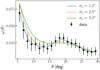 |
Fig. 4. Robustness test analyses. We performed small random shifts in the galaxies angular coordinates and repeated the 2PACF calculation. The black dots represent the original data analysis, and the curves correspond to the cases we studied (as indicated in the legend). |
4.4. Spectroscopic-z error
As shown by Sánchez et al. (2011), the main source of error in the BAO signal for photometric surveys is the uncertainty in the measurement of the redshift, z. Although we study spectroscopic data, for which this uncertainty is smaller, it is important to quantify this source of error in the final BAO measurement. To do this, we constructed 300 spec-z simulations for which we considered the measured z of each blue galaxy as the true one plus a random error obtained from a Gaussian distribution of zero mean and standard deviation given by its measured uncertainty that is available in the data catalog (see de Carvalho et al. 2020).
The results of this analysis are displayed in Fig. 5. There we show the histogram of the relative difference between the θFIT measured for each spec-z simulation and the θFIT from the blue galaxy data. As expected, in the case of spectroscopic data as for the blue galaxy data analyzed here, the error coming from the z-uncertainty introduces a small error in the final angular BAO measurement of 0.11%.
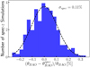 |
Fig. 5. Histogram of the relative difference, in percentage (%), between the BAO scale obtained from the blue galaxy data, θBAO, and those obtained from each simulated spec-z catalog, |

The 2D BAO measurement performed here complements a set of other measurements obtained with the same method (Carvalho et al. 2016, 2020; Alcaniz et al. 2017; de Carvalho et al. 2018). Thus, our angular BAO measurement at zeff = 0.11 is θBAO = 19.8°±1.05°. This error in the θBAO measurement includes the statistical and systematic errors due to the spectroscopic-z error, parameterization, RSD, projection effect, and nonlinearities (see Sánchez et al. 2011, for a broader discussion of the error estimation).
4.5. Cosmological constraints from θBAO data
Here we combined our 2D measurement of the BAO scale at low redshift, zeff = 0.11, with the results obtained by Carvalho et al. (2016), Alcaniz et al. (2017), de Carvalho et al. (2018) and Carvalho et al. (2020) (see Fig. 6), to constrain the parameters of the ΛCDM, wCDM, and w(t)CDM models. For the w(t)CDM model we chose the Barboza-Alcaniz parameterization (Barboza & Alcaniz 2008). To be consistent with the error determination from the analyses mentioned above and to allow a proper combination of the results, in this section we adopt σBAO = σFIT = 3.26° as the error in the measurement of θBAO, that is, θBAO(0.11) = 19.8° ± 3.26°.
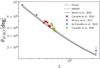 |
Fig. 6. θBAO measurements as a function of redshift. When the ΛCDM model is assumed, the dashed, dotted, and continuous lines represent the results obtained using the cosmological parameters from Planck Collaboration VI (2020), Hinshaw et al. (2013) (WMAP team), and Nunes et al. (2020), respectively. |
To restrict the cosmological parameters of the models ΛCDM, wCDM, and w(t)CDM, we performed Markov chain Monte Carlo (MCMC) analyses to explore the parameter space. In all cases we assumed Ωk = 0. The analyses were performed using the code PyMC5, assuming uniform priors for all the parameters in study except for rs, for which we assumed a Gaussian prior with a standard deviation equal to the measurement error. We investigated three different values of rs: rs = 99.08 ± 0.18 h−1 Mpc obtained by the Planck Collaboration VI (2020), rs = 106.61 ± 3.47 h−1 Mpc calculated by Hinshaw et al. (2013) (WMAP team), and rs = 102.2 ± 0.2 h−1 Mpc calculated by Nunes et al. (2020). The results of these analyses are displayed in Table 2, where the uncertainties correspond to 1σ errors. Figure 7 shows the constraints for ΛCDM model case as an example. The inner and the outer curves represent the 1σ and 2σ contour levels, respectively6. In the histogram plots, the ±1σ values are shown as dashed vertical lines. In all cases, the data prefer a high fraction of matter, with Ωm > 0.4. Moreover, the results from the wCDM and w(t)CDM models are consistent with the ΛCDM model, although the analyses reveal a poorer constraint of the parameters.
Constrained parameters for the models ΛCDM, wCDM, and w(t)CDM considering the sound horizon scale, rs, given by the Planck Collaboration VI (2020), WMAP Hinshaw et al. (2013), and Nunes et al. (2020).
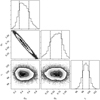 |
Fig. 7. Contour levels at 1σ (inner) and 2σ (outer) for the Ωm, ΩΛ and rs parameters extracted from the BAO angular scale data and the rs prior defined from the Planck value of Planck Collaboration VI (2020), namely rs = 99.08 ± 0.18 h−1 Mpc. In the histogram plots, the dashed vertical lines represent the ±1σ values. |
In general, we observe that the results are consistent with each other, but when the value from the Planck Collaboration, rs = 99.08 ± 0.18 h−1 Mpc, is used as a prior for rs, the constraints show the largest error bars (see Table 2). According to our tests, they are probably due to the small error of this parameter.
Finally, we calculated the angular diameter distance at zeff = 0.11. The angular scale of the BAO bump, θBAO(z), is related to the angular diameter distance DA(z) and the sound horizon rs by
 (9)
(9)
When we use our angular BAO measurement, θBAO(0.11) = 19.8° ± 1.05°, and the sound horizon scale calculated by the Planck Collaboration VI (2020), rs = 99.08 ± 0.18 h−1 Mpc, we use Eq. (9) to determine the angular diameter distance at zeff = 0.11: DA(0.11) = 258.31 ± 13.71 h−1 Mpc.
5. Conclusions
The availability of a rich set of astronomical data, mapping diverse cosmological tracers in various redshift intervals observed in large sky regions during long-time surveys makes these times exciting. This motivated us to study the BAO phenomenon in the local Universe, performing 2D statistical analyses of the low-redshift blue galaxy sample from the SDSS-DR12.
In the 2D clustering analyses performed here, we used a sample containing Ng = 15 942 blue galaxies in the thin redshift bin z ∈ [0.105, 0.115] with zeff = 0.11. Applying the 2PACF estimator on these data, we measured the transverse BAO signature at θBAO(0.11) = 19.8° ± 1.05° with a statistical significance of 2.2σ. Our error analyses included statistical and systematic contributions. We also performed analyses that confirm the robustness of this transverse BAO measurement (see Sect. 4.3 for details).
Additionally, we used the sound horizon scale calculated by the Planck Collaboration VI (2020), rs = 99.08 ± 0.18 h−1 Mpc, to obtain a measurement of the angular diameter distance. Using this value of rs and our result for the BAO angular scale θBAO(0.11) in Eq. (9), we obtained a measurement of the angular diameter distance at zeff = 0.11: DA(0.11)=258.31 ± 13.71 h−1 Mpc. For the error analyses, which requires the computation of the covariance matrices, we used a set of log-normal simulations with similar observational features as the SDSS data we analyzed, including effects such as lensing, RSD, and nonlinear clustering (see Sect. 2.2 for details).
Our measurement of DA(0.11) was obtained by applying a method that is weakly dependent on a cosmological model, exactly as other measurements of DA(z) were obtained (Carvalho et al. 2016, 2020; Alcaniz et al. 2017; de Carvalho et al. 2018). Here we used these measurements to perform MCMC analyses that constrain cosmological parameters of some ΛCDM-type models, namely ΛCDM itself, wCDM, and w(t)CDM. The results we obtained are shown in Table 2 and Fig. 7. They agree with the reported values for these models (for analyses of cosmological parameters, see, e.g., Hinshaw et al. 2013; Planck Collaboration VI 2020; Marques et al. 2019; Nunes et al. 2020; Nunes & Bernui 2020).
Here α is also accounted for as a free parameter, that is, we have a total of four and seven free parameters in the non-BAO and BAO cases, respectively.
This figure was made using the Corner Plot software developed by Foreman-Mackey (2016).
Acknowledgments
The authors thank the Brazilian agencies PROPG-CAPES/FAPEAM program, CNPq, CAPES, and FAPESP for the grants under which this work was carried out.
References
- Abbott, T., Abdalla, F., Alarcon, A., et al. 2019, MNRAS, 483, 4866 [CrossRef] [Google Scholar]
- Alam, S., Albareti, F. D., Prieto, C. A., et al. 2015, ApJS, 219, 12 [NASA ADS] [CrossRef] [Google Scholar]
- Alam, S., Ata, M., Bailey, S., et al. 2017, MNRAS, 470, 2617 [NASA ADS] [CrossRef] [Google Scholar]
- Alam, S., Aubert, M., Avila, S., et al. 2020, ArXiv e-prints [arXiv:2007.08991] [Google Scholar]
- Alcaniz, J. S., Carvalho, G. C., Bernui, A., et al. 2017, Grav. Quantum Fundam. Theor. Phys., 187, 11 [Google Scholar]
- Avila, F., Novaes, C. P., Bernui, A., & de Carvalho, E. 2018, J. Cosmol. Astropart. Phys., 12, 041 [Google Scholar]
- Avila, F., Novaes, C. P., Bernui, A., de Carvalho, E., & Nogueira-Cavalcante, J. P. 2019, MNRAS, 488, 1481 [NASA ADS] [CrossRef] [Google Scholar]
- Barboza, E., & Alcaniz, J. S. 2008, Phys. Lett. B, 666, 415 [NASA ADS] [CrossRef] [Google Scholar]
- Bassett, B., & Hlozek, R. 2010, Baryon Acoustic Oscillations, in Dark Energy Observational and Theoretical Approaches (Cambridge Univ. Press), 246 [Google Scholar]
- Bengaly, C. A. P., Bernui, A., Ferreira, I. S., & Alcaniz, J. S. 2017, MNRAS, 466, 2799 [NASA ADS] [CrossRef] [Google Scholar]
- Beutler, F., Blake, C., Colless, M., et al. 2011, MNRAS, 416, 3017 [Google Scholar]
- Blake, C., Kazin, E. A., Beutler, F., et al. 2011, MNRAS, 418, 1707 [NASA ADS] [CrossRef] [MathSciNet] [Google Scholar]
- Bond, J. R., & Efstathiou, G. 1987, MNRAS, 226, 655 [NASA ADS] [Google Scholar]
- Carnero, A., Sánchez, E., Crocce, M., Cabré, A., & Gaztanaga, E. 2012, MNRAS, 419, 1689 [NASA ADS] [CrossRef] [Google Scholar]
- Carter, P., Beutler, F., Percival, W. J., et al. 2018, MNRAS, 481, 2371 [Google Scholar]
- Carvalho, G. C., Bernui, A., Benetti, M., Carvalho, J. C., & Alcaniz, J. S. 2016, Phys. Rev. D, 93 [Google Scholar]
- Carvalho, G. C., Bernui, A., Benetti, M., et al. 2020, Astropart. Phys., 119 [Google Scholar]
- Challinor, A., & Lewis, A. 2011, Phys. Rev. D, 84, 043516 [NASA ADS] [CrossRef] [Google Scholar]
- Cole, S., Percival, W. J., Peacock, J. A., et al. 2005, MNRAS, 362, 505 [NASA ADS] [CrossRef] [Google Scholar]
- de Carvalho, E., Bernui, A., Carvalho, G. C., Novaes, C. P., & Xavier, H. S. 2018, J. Cosmol. Astropart. Phys., 04, 064 [CrossRef] [Google Scholar]
- de Carvalho, E., Bernui, A., Xavier, H. S., & Novaes, C. P. 2020, MNRAS, 492, 4469 [NASA ADS] [CrossRef] [Google Scholar]
- Eisenstein, D. J., & Hu, W. 1998, ApJ, 496, 605 [NASA ADS] [CrossRef] [Google Scholar]
- Eisenstein, D. J., Zehavi, I., Hogg, D. W., et al. 2005, ApJ, 633, 560 [Google Scholar]
- Eisenstein, D. J., Seo, H.-J., & White, M. 2007, ApJ, 664, 660 [NASA ADS] [CrossRef] [Google Scholar]
- Feldbrugge, J., van Engelen, M., van de Weygaert, R., Pranav, P., & Vegter, G. 2019, J. Cosmol. Astropart. Phys., 09, 052 [CrossRef] [Google Scholar]
- Feldman, H. A., Kaiser, N., & Peacock, J. A. 1994, ApJ, 426, 23 [NASA ADS] [CrossRef] [Google Scholar]
- Foreman-Mackey, D. 2016, J. Open Source Soft., 1 [Google Scholar]
- Górski, K. M., Hivon, E., Banday, A. J., et al. 2005, ApJ, 622, 759 [NASA ADS] [CrossRef] [Google Scholar]
- Hinshaw, G., Larson, D., Komatsu, E., et al. 2013, ApJS, 208, 19 [Google Scholar]
- Jarvis, M., Bernstein, G., & Jain, B. 2004, MNRAS, 352, 338 [Google Scholar]
- Kaiser, N. 1987, MNRAS, 227, 1 [Google Scholar]
- Landy, S. D., & Szalay, A. S. 1993, ApJ, 412, 64 [Google Scholar]
- Marques, G. A., & Bernui, A. 2020, J. Cosmol. Astropart. Phys., 05, 052 [CrossRef] [Google Scholar]
- Marques, G. A., Liu, J., Zorrilla Matilla, J. M., et al. 2019, J. Cosmol. Astropart. Phys., 06, 019 [CrossRef] [Google Scholar]
- Marques, G. A., Liu, J., Huffenberger, K. M., & Colin, H. J. 2020, ApJ, 904, 182 [Google Scholar]
- Novaes, C. P., Bernui, A., Marques, G. A., & Ferreira, I. S. 2016, MNRAS, 461, 1363 [NASA ADS] [CrossRef] [Google Scholar]
- Novaes, C. P., Bernui, A., Xavier, H. S., & Marques, G. A. 2018, MNRAS, 478, 3253 [NASA ADS] [CrossRef] [Google Scholar]
- Nunes, R. C., & Bernui, A. 2020, EPJC, 80, 1025 [NASA ADS] [CrossRef] [EDP Sciences] [Google Scholar]
- Nunes, R. C., Yadav, S. K., Jesus, J. F., & Bernui, A. 2020, MNRAS, 497, 2 [Google Scholar]
- Pandey, B., & Sarkar, S. 2020, MNRAS, 498, 6069 [NASA ADS] [CrossRef] [Google Scholar]
- Peebles, P. J. E., & Hauser, M. G. 1974, ApJS, 28, 19 [NASA ADS] [CrossRef] [Google Scholar]
- Peebles, P. J. E., & Yu, J. T. 1970, ApJ, 162, 815 [NASA ADS] [CrossRef] [Google Scholar]
- Planck Collaboration VI. 2020, A&A, 641, A6 [NASA ADS] [CrossRef] [EDP Sciences] [Google Scholar]
- Sánchez, E., Carnero, A., Garcia-Bellido, J., et al. 2011, MNRAS, 411, 277 [Google Scholar]
- Salazar-Albornoz, S., Sánchez, A. G., Grieb, J. N., et al. 2017, MNRAS, 468, 2938 [Google Scholar]
- Sosa Nuñez, F., & Niz, G. 2020, J. Cosmol. Astropart. Phys., 12, 021 [Google Scholar]
- Sunyaev, R. A., & Zeldovich, Y. B. 1970, Astrophys. Space Sci., 7, 3 [Google Scholar]
- Xavier, H. S., Abdalla, F. B., & Joachimi, B. 2016, MNRAS, 459, 3693 [Google Scholar]
- York, D. G., Adelman, J., Anderson, J. E., et al. 2000, AJ, 120, 1579 [CrossRef] [Google Scholar]
All Tables
Constrained parameters for the models ΛCDM, wCDM, and w(t)CDM considering the sound horizon scale, rs, given by the Planck Collaboration VI (2020), WMAP Hinshaw et al. (2013), and Nunes et al. (2020).
All Figures
|
Fig. 1. Sample of SDSS blue galaxies in equatorial coordinates J2000 (in degrees). |
| In the text | |
|
Fig. 2. BAO signature obtained in the 2PACF by analyzing the sample in the redshift interval z ∈ [0.105, 0.115], with δz = 0.01. The bin size in this 2PACF is 1.25°, and we use 50 random catalogs with the same observational features as the galaxy catalog. |
| In the text | |
|
Fig. 3. Covariance matrix for the 2PACF obtained from Eq. (4) using the set of log-normal simulated maps (see Sect. 2.2). |
| In the text | |
|
Fig. 4. Robustness test analyses. We performed small random shifts in the galaxies angular coordinates and repeated the 2PACF calculation. The black dots represent the original data analysis, and the curves correspond to the cases we studied (as indicated in the legend). |
| In the text | |
|
Fig. 5. Histogram of the relative difference, in percentage (%), between the BAO scale obtained from the blue galaxy data, θBAO, and those obtained from each simulated spec-z catalog, |
| In the text | |
|
Fig. 6. θBAO measurements as a function of redshift. When the ΛCDM model is assumed, the dashed, dotted, and continuous lines represent the results obtained using the cosmological parameters from Planck Collaboration VI (2020), Hinshaw et al. (2013) (WMAP team), and Nunes et al. (2020), respectively. |
| In the text | |
|
Fig. 7. Contour levels at 1σ (inner) and 2σ (outer) for the Ωm, ΩΛ and rs parameters extracted from the BAO angular scale data and the rs prior defined from the Planck value of Planck Collaboration VI (2020), namely rs = 99.08 ± 0.18 h−1 Mpc. In the histogram plots, the dashed vertical lines represent the ±1σ values. |
| In the text | |
Current usage metrics show cumulative count of Article Views (full-text article views including HTML views, PDF and ePub downloads, according to the available data) and Abstracts Views on Vision4Press platform.
Data correspond to usage on the plateform after 2015. The current usage metrics is available 48-96 hours after online publication and is updated daily on week days.
Initial download of the metrics may take a while.