| Issue |
A&A
Volume 648, April 2021
|
|
|---|---|---|
| Article Number | L8 | |
| Number of page(s) | 4 | |
| Section | Letters to the Editor | |
| DOI | https://doi.org/10.1051/0004-6361/202140837 | |
| Published online | 26 April 2021 | |
Letter to the Editor
Evidence for SO2 latitudinal variations below the clouds of Venus
1
LATMOS/IPSL, UVSQ Université Paris-Saclay, Sorbonne Université, CNRS, Guyancourt, France
e-mail: emmanuel.marcq@latmos.ipsl.fr
2
LESIA, Observatoire de Paris, Université PSL, CNRS, Sorbonne Université, Université de Paris, 5 place Jules Janssen, 92195 Meudon, France
Received:
19
March
2021
Accepted:
14
April
2021
Context. Sulphur dioxide (SO2) is highly variable above the clouds of Venus, yet no spatial or temporal variability below the clouds had been known until now.
Aims. In order to constrain Venus’s atmospheric circulation and chemistry (including possible volcanic outgassing), more accurate SO2 measurements below the clouds are therefore needed.
Methods. We used the high-resolution iSHELL spectrometer located at the NASA IRTF to record thermal night-side spectra, which we fitted using an updated forward radiative transfer model that was previously employed to process SpeX/IRTF and VIRTIS-H/Venus Express spectra.
Results. We report, for the first time, an increase in SO2 with increasing latitude (+30% between the minimum near 15°S and > 35°N). This is consistent with the interaction between the Hadley-cell circulation and a postulated vertical profile in SO2 estimated to increase between 30 and 40 km in altitude, as previously suggested by in situ ISAV measurements.
Conclusions. This SO2 variability challenges our current understanding of Venus’s tropospheric thermochemistry and underlines the high scientific return from high-resolution spectroscopy from, for example, future orbiters.
Key words: planets and satellites: atmospheres / techniques: spectroscopic
© E. Marcq et al. 2021
 Open Access article, published by EDP Sciences, under the terms of the Creative Commons Attribution License (https://creativecommons.org/licenses/by/4.0), which permits unrestricted use, distribution, and reproduction in any medium, provided the original work is properly cited.
1. Introduction
Although sulphur dioxide (SO2) is known to vary by several orders of magnitude at the cloud top of Venus (Esposito 1984; Esposito et al. 1988; Marcq et al. 2013, 2020; Vandaele et al. 2017a,b), such a variability could never be evidenced in the troposphere below the clouds, mostly since remote measurements rely on the sole spectroscopic analysis of a narrow spectral feature in the night-side thermal emission of Venus near 2.46 μm (Bézard et al. 1993). Various spectroscopic analyses of this night-side emission have led to the commonly accepted range for the SO2 mixing ratio of 130 ± 50 ppmv (Marcq et al. 2008; Arney et al. 2014; Vandaele et al. 2017b). Yet, in order to understand SO2 variability above the clouds, and possibly relate it to volcanic outgassing (Esposito 1984), its behaviour in the troposphere (which acts as a proximal reservoir for cloud-top SO2) must be better characterised. Investigations using high-spectral-resolution observations provide a means to achieve this goal since they allow for a better separation between the various minor gaseous species absorbing in the 2.3 − 2.5 μm near-infrared window, namely: CO, OCS, H2O, HDO, and HF (Taylor et al. 1997). To address this, we performed new high-spectral-resolution observations, which are described in Sect. 2. We compare them to our radiative transfer calculations in Sect. 3. We present our co-located SO2 and CO measurements and discuss their implications in Sect. 4, before summarising our findings in the last section, Sect. 5.
2. Observations
2.1. Acquisition
We performed our observations in January 2019 and August 2020, during western elongations of Venus (another observation campaign was scheduled in late April 2020 during an eastern elongation but could not be performed since the Mauna Kea observatory was closed due to the COVID-19 pandemic). We used the infrared high-resolution iSHELL echelle spectrograph (Rayner et al. 2016) mounted at the NASA Infrared Telescope Facility (IRTF) in Hawaii. We chose to use the 5″ × 1.5″ slit as a compromise between minimising acquisition time on the night side of Venus and limiting stray-light contamination from the day side of Venus. In the K3 grating mode of iSHELL, the spectral interval ranges from 2.26 μm to 2.55 μm, covering the longer wavelength portion of the 2.2 − 2.5 μm thermal infrared window of Venus, and extending beyond at longer wavelengths.
Since the angular diameter of Venus during maximal elongations far exceeds 5″, we also recorded images from the guider at 3.46 μm to avoid saturation and properly locate the day side of Venus, including the terminator. These guider images were then compared to ephemeris computations from the Institut de mécanique céleste et de calcul des éphémérides (IMCCE) in order to properly locate the slit geometry projected on the Venusian disk (latitude, local time, emission angle). The slit was always kept parallel to the terminator.
During each session, we recorded (1) spectra from standard A stars used for intensity calibration by the SpeXTool suite, (2) spectra recorded on the night side of Venus, (3) spectra recorded on the day side of Venus, and (4) sky images for background subtraction. Stellar spectra were recorded early during each session, when the sky was dark enough and Venus was too low on the horizon to observe, and at a similar airmass to later Venus observations. The typical required integration time is close to 30 min for a slit position on the night side, 2 min on the day side, and 10 min for calibration stars (see Table 1).
Observation summary.
2.2. Processing
As previously mentioned, we performed the first stages of our data processing using the SpeXTool data reduction package (Cushing et al. 2004; Vacca et al. 2003). In order to increase the signal-to-noise ratio (S/N) and considering the typical seeing extent (∼1″), we divided each slit position on the night side into two separate 2″ × 1.5″ locations. The SpeXTool package provides calibrated spectra, in both wavelength and spectral radiance, as well as error intervals for each of the 27 dispersion orders of the echelle grating.
Following our past IRTF observations of Venus using SpeX (Marcq et al. 2005, 2006), we cleaned the night-side thermal emission spectra from the day-side solar stray light by subtracting a day-side spectrum acquired near the terminator. The day-side spectrum was interpolated using several day-side observations in order to match the same terrestrial airmass as the night-side observation. The amount of stray light to subtract was determined by taking advantage of the saturation of spectrally resolved CO lines in the 2.32 − 2.35 μm interval (Fig. 1) since telluric absorption is too strong to make use of wavelengths longer than 2.5 μm. Data were then filtered by removing outliers (resulting from the faulty correction of some telluric absorption lines by SpeXTool) and then spectrally smoothed in order to increase the S/N while keeping our effective spectral resolution close to λ/Δλ ≃ 20 000.
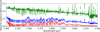 |
Fig. 1. Raw night-side spectrum (blue), interpolated day-side spectrum (×0.05, green), and resulting cleaned night-side spectrum (red) acquired on January 3, 2019. |
3. Fitting
3.1. Forward radiative transfer model
We employed an updated version of the radiative transfer model previously used by Marcq et al. (2005, 2006, 2008). The two main updates are the following: (1) An eight-stream radiative transfer solver based on DISORT (Stamnes et al. 1988) was used, which allowed us to take the effect of a variation in emission angle into account; and (2) the CO2 line database was updated using the ab initio list from Huang et al. (2014).
3.1.1. Limb darkening
We found that our model yields a remarkably simple wavelength-independent limb darkening parametrisation: I(μ) = I(μ = 1) × (0.74μ + 0.26), where μ stands for the cosine of the emission angle. This is easily understood considering the strong multiple scattering in the optically thick clouds above the emission region and the very small opacity of the atmosphere above the clouds.
3.1.2. Vertical profiles of gaseous species
Our updated model uses the same method of specifying the vertical profiles of minor species as in Marcq et al. (2008): Volume mixing ratios (qi) are specified for a limited number of pressure levels (Pi), and the mixing ratios are linearly interpolated (in log q vs. log P coordinates) in between. The nominal qi(Pi) values are given in Table 2 for CO and SO2.
Nominal vertical profiles for CO and SO2.
3.2. Fitting algorithm
The fitting algorithm proceeds in two stages; a Levenberg-Marquardt loop (Newville et al. 2014) interpolating from look-up tables computed by the forward radiative transfer model described in Sect. 3.1 is used in both. In the first stage, lower cloud opacity and a carbon monoxide scaling factor are retrieved using grating orders 13 to 19 (2.325 to 2.402 μm) and assuming the same CO vertical profile shape as Marcq et al. (2008). In the second stage, assuming the previously retrieved CO and lower cloud opacity values and using grating orders 7 to 10 (2.422 to 2.470 μm), OCS mixing ratios at 30 and 37 km are retrieved, as is an SO2 scaling factor. A typical fit is shown in Fig. 2.
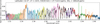 |
Fig. 2. Spectrum observed on January 3, 2019 (colour coding for the different, partially overlapping grating orders) and its best fit (in black). The grey shaded area near 2.46 μm shows the sensitivity to the SO2 mixing ratio (shaded between ×2 and ×0.5 the best fit value). |
4. Results
4.1. Carbon monoxide (CO)
Our retrievals for CO are shown in Fig. 3. These results are in agreement with previous measurements (Marcq et al. 2018): Carbon monoxide increases with increasing latitude, although the latitude of minimum CO is shifted to circa 15°S. Such a shift was also seen by previous observers (Marcq et al. 2008; Arney et al. 2014) and interpreted as the influence of topography (especially in Aphrodite Terra) on the large-scale circulation, which is responsible for creating this latitudinal gradient – CO being produced photochemically at higher altitudes and carried below the cloud through the downwelling branch of the Hadley cell (Tsang et al. 2008).
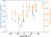 |
Fig. 3. CO and SO2 volume mixing ratio measurements. Error bars stand for ±3 ⋅ σ standard deviations. Systematic uncertainties of the absolute SO2 mixing ratio are not displayed. |
Additionally, this shift makes our observed CO distribution less correlated with the emission angle than for a hemispherically symmetric CO distribution. It is therefore less likely that it originates from a faulty limb darkening correction, which further increases our confidence in these results.
4.2. Sulphur dioxide (SO2)
Our co-located retrievals for SO2 are also shown in Fig. 3. Previous measurements suffered very large error bars due to the narrowness of SO2 spectral features near 2.46 μm, and they agreed on a latitudinally constant value of 130 ± 50 ppmv below the clouds (Vandaele et al. 2017a; Marcq et al. 2018). Very interestingly, Arney et al. (2014, their Fig. 26) observed a quantitatively similar pattern in their SO2 maps but dismissed it on the basis of the large error bars and other ‘ghosting effects’ inherent to their low-to-medium spectral resolution. However, our high-resolution iSHELL observations circumvent this issue, such that an increase in SO2 with increasing latitude is unambiguous in our data. Interestingly, the latitudinal offset is the same as for CO, hinting at a common mechanism behind these variations, which is further discussed in Sect. 4.3.
We also note that our latitudinally averaged value is closer to 180 ppmv, 40% higher than the commonly accepted value. However, we found that this average value depends on several factors, such as the assumed CO2-CO2 continuum value, the parametrisation of cloud opacity, and the exact amount of stray light that is subtracted. On the other hand, relative variations are much better constrained, and so we focus on this new result hereafter.
4.3. Discussion
The aforementioned correlation (R2 ≃ 0.694) between SO2 and CO can be seen in Fig. 4 and hints at a common origin for their horizontal variability. For CO, this tropospheric variability comes from the competition between the positive vertical gradient (itself originating from the relative altitude of its photochemical source, which is located above the sounded altitude, and a lower atmospheric sink, which is located below) and the general Hadley-cell circulation (Tsang et al. 2008). We therefore infer that SO2 should also exhibit a positive vertical gradient below the clouds in order to account for its observed latitudinal variability. We can even estimate the typical value of the required vertical gradient based on the already known CO gradient value, assuming there are no sources or sinks for either species and that the probed altitudes are similar: Since the typical gradient for CO is close to +1 ppm km−1 (Marcq et al. 2018), we estimate a SO2 vertical gradient of the order of +10 ppm km−1 in the probed altitude range.
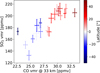 |
Fig. 4. Correlation plot between CO and SO2 measurements. Error bars stand for ±3 ⋅ σ standard deviations, and colour is coded for the measurement latitudes. Systematic uncertainties of the absolute SO2 mixing ratio are not displayed. |
Coincidentally, this gradient value is close to the value found by in situ ISAV measurements on board VEGA descent probes (Bertaux et al. 1996), though ISAV measured substantially lower mixing ratios for SO2 than what we found. However, currently available thermochemical models of the lower atmosphere (Krasnopolsky 2007) do not predict such a vertical gradient (even suggesting a moderate decrease in the 30 − 40 km altitude range). Further modelling work is definitely required in order to account for this newly discovered SO2 variability.
5. Conclusion
Our iSHELL observations of the night-side thermal spectra of Venus showed, for the first time, an increase in SO2 with increasing latitude below the clouds of Venus, which we tentatively ascribe to the general circulation acting on an increasing-with-height SO2 mixing ratio. This study also highlights the interest of high-spectral-resolution infrared spectra for accurate measurements of trace gases in Venus’s atmosphere, either from long-term-monitoring ground-based instruments, such as iSHELL, or dedicated space-borne instruments, such as the VenSpec-H channel (Robert et al., in prep.) on board ESA M5 candidate EnVision.
Acknowledgments
E. Marcq wishes to thank L. Bercot for his logistic support during remote IRTF observations in August 2020, as well as A. Boogert, G. Osterman, G. Engh, and J. Rayner for their support during iSHELL operations in both 2019 and 2020 observations campaigns. The authors also thank C. F. Wilson for his valuable comments and remarks.
References
- Arney, G., Meadows, V., Crisp, D., et al. 2014, J. Geophys. Res.: Planets, 119, 1860 [Google Scholar]
- Bertaux, J., Widemann, T., Hauchecorne, A., Moroz, V. I., & Ekonomov, A. P. 1996, J. Geophys. Res, 101, 12709 [Google Scholar]
- Bézard, B., de Bergh, C., Fegley, B., et al. 1993, Geophys. Res. Lett., 20, 1587 [Google Scholar]
- Cushing, M. C., Vacca, W. D., & Rayner, J. T. 2004, PASP, 116, 362 [Google Scholar]
- Esposito, L. W. 1984, Science, 223, 1072 [Google Scholar]
- Esposito, L. W., Copley, M., Eckert, R., et al. 1988, J. Geophys. Res., 93, 5267 [Google Scholar]
- Huang, X., Gamache, R. R., Freedman, R. S., Schwenke, D. W., & Lee, T. J. 2014, J. Quant. Spectr. Rad. Transf., 147, 134 [Google Scholar]
- Krasnopolsky, V. A. 2007, Icarus, 191, 25 [Google Scholar]
- Marcq, E., Bézard, B., Encrenaz, T., & Birlan, M. 2005, Icarus, 179, 375 [Google Scholar]
- Marcq, E., Encrenaz, T., Bézard, B., & Birlan, M. 2006, Planet. Space Sci., 54, 1360 [Google Scholar]
- Marcq, E., Bézard, B., Drossart, P., et al. 2008, J. Geophys. Res.: Planets, 113, E00B07 [Google Scholar]
- Marcq, E., Bertaux, J.-L., Montmessin, F., & Belyaev, D. 2013, Nature Geosci., 6, 25 [Google Scholar]
- Marcq, E., Mills, F. P., Parkinson, C. D., & Vandaele, A. C. 2018, Space Sci. Rev., 214, 10 [Google Scholar]
- Marcq, E., Lea Jessup, K., Baggio, L., et al. 2020, Icarus, 335, 113368 [Google Scholar]
- Newville, M., Stensitzki, T., Allen, D. B., & Ingargiola, A. 2014, https://doi.org/10.5281/zenodo.11813 [Google Scholar]
- Rayner, J. T., Tokunaga, A., Jaffe, D., et al. 2016, SPIE Conf. Ser., 9908E, 84R [Google Scholar]
- Stamnes, K., Tsay, S., Jayaweera, K., & Wiscombe, W. 1988, Appl. Opt., 27, 2502 [Google Scholar]
- Taylor, F. W., Crisp, D., & Bézard, B. 1997, in Venus II, eds. D. M. Hunten, L. Glin, T. M. Donahue, & V. I. Moroz (Tucson: University of Arizona Press), 325 [Google Scholar]
- Tsang, C. C. C., Irwin, P. G. J., Wilson, C. F., et al. 2008, J. Geophys. Res.: Planets, 113, E00B08 [Google Scholar]
- Vacca, W. D., Cushing, M. C., & Rayner, J. T. 2003, PASP, 115, 389 [Google Scholar]
- Vandaele, A. C., Korablev, O., Belyaev, D., et al. 2017a, Icarus, 295, 16 [Google Scholar]
- Vandaele, A. C., Korablev, O., Belyaev, D., et al. 2017b, Icarus, 295, 1 [Google Scholar]
All Tables
All Figures
|
Fig. 1. Raw night-side spectrum (blue), interpolated day-side spectrum (×0.05, green), and resulting cleaned night-side spectrum (red) acquired on January 3, 2019. |
| In the text | |
|
Fig. 2. Spectrum observed on January 3, 2019 (colour coding for the different, partially overlapping grating orders) and its best fit (in black). The grey shaded area near 2.46 μm shows the sensitivity to the SO2 mixing ratio (shaded between ×2 and ×0.5 the best fit value). |
| In the text | |
|
Fig. 3. CO and SO2 volume mixing ratio measurements. Error bars stand for ±3 ⋅ σ standard deviations. Systematic uncertainties of the absolute SO2 mixing ratio are not displayed. |
| In the text | |
|
Fig. 4. Correlation plot between CO and SO2 measurements. Error bars stand for ±3 ⋅ σ standard deviations, and colour is coded for the measurement latitudes. Systematic uncertainties of the absolute SO2 mixing ratio are not displayed. |
| In the text | |
Current usage metrics show cumulative count of Article Views (full-text article views including HTML views, PDF and ePub downloads, according to the available data) and Abstracts Views on Vision4Press platform.
Data correspond to usage on the plateform after 2015. The current usage metrics is available 48-96 hours after online publication and is updated daily on week days.
Initial download of the metrics may take a while.