| Issue |
A&A
Volume 648, April 2021
|
|
|---|---|---|
| Article Number | A111 | |
| Number of page(s) | 6 | |
| Section | Stellar structure and evolution | |
| DOI | https://doi.org/10.1051/0004-6361/202140489 | |
| Published online | 22 April 2021 | |
Rotationally and tidally distorted compact stars
A theoretical approach to the gravity-darkening exponents for white dwarfs
1
Instituto de Astrofísica de Andalucía, CSIC, Apartado 3004, 18080 Granada, Spain
e-mail: This email address is being protected from spambots. You need JavaScript enabled to view it.
2
Dept. Física Teórica y del Cosmos, Universidad de Granada, Campus de Fuentenueva s/n, 10871 Granada, Spain
Received:
3
February
2021
Accepted:
26
February
2021
Abstract
Context. To the best of our knowledge, there are no specific calculations of gravity-darkening exponents for white dwarfs in the literature. On the other hand, the number of known eclipsing binaries whose components are tidally and/or rotationally distorted white dwarfs is increasing year on year.
Aims. Our main objective is to present the first theoretical approaches to the problem of the distribution of temperatures on the surfaces of compact stars distorted by rotation and/or tides in order to compare with relevant observational data.
Methods. We used two methods to calculate the gravity-darkening exponents: (a) a variant of our numerical method based on the triangles strategy and (b) an analytical approach consisting in a generalisation of the von Zeipel theorem for hot white dwarfs.
Results. We find discrepancies between the gravity-darkening exponents calculated with our methods and the predictions of the von Zeipel theorem, particularly in the cases of cold white dwarfs; although the discrepancy also applies to higher effective temperatures under determined physical conditions. We find physical connections between the gravity-darkening exponents calculated using our modified method of triangles strategy with the convective efficiency (defined here as the ratio of the convective to the total flux). A connection between the entropy and the gravity-darkening coefficients is also found: variations of the former cause changes in the way the temperature is distributed on distorted stellar surfaces. On the other hand, we have generalised the von Zeipel theorem for the case of hot white dwarfs. Such a generalisation allows us to predict that, under certain circumstances, the value of the gravity-darkening exponent may be smaller than 1.0, even in the case of high effective temperatures.
Conclusions. To constrain the gravity-darkening exponent values observationally it would be necessary to find and investigate eclipsing binaries constituted by white dwarfs showing tidal and/or rotational distortions that were double-lined and that were bright enough to obtain good radial-velocity semi-amplitudes for both components. It would be very interesting and useful if observer were to focus their attention on this kind of system to check our theoretical results.
Key words: binaries: general / binaries: eclipsing / white dwarfs / stars: atmospheres
© ESO 2021
1. Introduction
Gravity-darkening is an important piece of the stellar structure and evolution that has been studied for almost a hundred years (von Zeipel 1924). Gravity-darkening exponents (GDE) are key tools for analysing light curves of eclipsing binaries or in isolated rotating stars through long-baseline optical and infrared interferometry. Considering stars in strict radiative equilibrium (pseudo-barotrope), in 1924 von Zeipel showed that the variation of brightness over the surface is proportional to the effective gravity, that is,
 (1)
(1)
or equivalently
 (2)
(2)
where ψ is the potential, g the local gravity, T the local temperature, κ the opacity, ρ the local density, a the radiation pressure constant, c the velocity of light in vacuum, Teff the effective temperature, and β1 = 1.0 is the GDE, which is a bolometric quantity. Although we are still far from fully understanding the gravity-darkening phenomenon, in the last 22 years several theoretical papers related to the GDE have appeared in the literature that have shed some light on the scenario, such as Claret (1998, 2000, 2012), Espinosa Lara & Rieutord (2011, 2012), and McGill et al. (2013). For a historical summary of the theoretical research on the GDE see Claret (1998, 2016). From now on we also designate the GDE as β1.
Another important and complementary ingredient in the analysis of systems with non-spherical configurations are the so-called gravity-darkening coefficients (GDCs). As we can only observe determined band-limited stellar flux (not the bolometric), the introduction of these coefficients is necessary in order to model a distorted star. Such a coefficient can be written as (Claret & Bloemen 2011):
![Mathematical equation: $$ \begin{aligned}&{ y}(\lambda , T_{\rm eff}, \log \mathrm{[A/H]}, \log g, V_{\xi }) \nonumber \\&\quad =\left(\frac{\mathrm{d}\ln T_{\rm eff }}{{\mathrm{d}\ln g}}\right) \left(\frac{\partial {\ln I_o(\lambda )}}{{\partial {\ln T_{\rm eff }}}}\right)_{g} + \left(\frac{\partial {\ln I_o(\lambda )}}{\partial {\ln g}}\right)_{T_{\rm eff}}, \end{aligned} $$](/articles/aa/full_html/2021/04/aa40489-21/aa40489-21-eq3.gif) (3)
(3)
where λ is the wavelength, Io(λ) the intensity at a given wavelength at the centre of the stellar disc, and Vξ is the microturbulent velocity. We note that the expression  can be written as β1/4. In order to progress in our investigation of stellar configurations distorted by rotation and/or tides, we recently studied the GDCs for the case of compact stars (Claret et al. 2020). In that study we computed GDC for DA, DB, and DBA white dwarf models, covering the transmission curves of the Sloan, UBVRI, Kepler, TESS, Gaia, and HiPERCAM photometric systems. These computations are available for log [H/He] = −10.0 (DB), −2.0 (DBA), and He/H = 0 (DA). The covered range of log g was 5.0–9.5, while for the effective temperatures the respective range was 3750 K–100 000 K.
From an observational point of view, discoveries of binary systems whose components are tidally and/or rotationally distorted white dwarfs are ongoing (see e.g. Burdge et al. 2019a,b, 2020; Kupfer et al. 2020 and references therein). However, as far as we know, there are no specific GDE calculations for white dwarf sequences or even for an individual model. In this short paper we present, for the first time, GDEs for three white dwarf cooling sequences. We also introduce some improvements to our methods for calculating the GDE: β1 is computed as a function of the optical depth, that is, β1 = β1(τ). In addition, we introduce an extra condition in our calculations, namely the relationship between the local gravities and the corresponding optical depths for a given equipotential surface. In the following, sections we discuss these points in more detail.
The paper is organised as follows: Sect. 2 is dedicated to describing our methods and some aspects of the distorted stellar configurations. In Sect. 3 we discuss both observational and theoretical evidence for deviations from von von Zeipel’s theorem (1924) and present our results and conclusions.
2. The numerical method
Our numerical method is based on the triangles strategy introduced by Kippenhahn et al. (1967). A complete description of our method can be found in Claret (1998), but for the sake of clarity, we summarise it below. To save computing time, Kippenhahn et al. (1967) introduced an ingenious method: when an evolutionary sequence is being calculated, if the external boundary conditions are unchanged at the fitting point (envelope-interior), the outer layer integrations must be the same as the previous ones. Three envelopes corresponding to three points in the Hertzsprung-Russell (HR) diagram around the current values of luminosity and effective temperature are computed. As the model evolves, its properties are checked to see if they remain within this triangle. If so, the boundary conditions are unchanged. It is important to highlight that this strategy is valid only if the triangle is sufficiently small. This warning is particularly valid for convective envelopes. To simulate a distorted star, we are interested in several triangles showing different effective temperature distributions over the surface. Therefore, we increase the number of triangles in the HR diagram, that is, we compute several envelopes with different temperature distributions but imposing the same physical conditions at a given interior point. Figure 2 in Claret (2000) shows a simplified scheme of our method where only three points are shown in the HR diagram. Once the triangles have been computed for each point of the evolutionary track we can derive β1 by differentiating the neighbouring envelopes. Such a procedure is performed for the next evolutionary track point and so on.
Our method has some advantages: (a) it can be applied to convective and/or radiative envelopes; (b) one can investigate the influence of the optical depth in the GDE by changing the fitting point to impose the boundary conditions, without loss of generality; (c) the GDE can be computed as a function of initial mass, chemical composition, evolutionary stage (in the present paper up to the white dwarf phase), and other ingredients of the input physics, and (d) more realistic atmosphere models can easily be incorporated as external boundary conditions, as done in Claret (2012).
We introduce an extra condition in our procedure: the relationship between local gravity and optical depth over a given equipotential surface. In reality, solving the hydrostatic equilibrium equation for two points on an equipotential characterised by [g(μ),τ(μ, ψ)], we obtain g(μ)τ(μ, ψ) = g(μo)τ(μo, ψ). In this relationship, g is the local gravity, ψ is the total potential (rotational one included), τ is the optical depth, and μ is given by cos(ϕ) where ϕ is the angle between the radiation field and the z axis. The subscript o indicates the reference point, for example the pole. To guarantee that the triangle technique represents an equipotential, we have taken as reference the absolute dimensions for each point of the evolutionary models, that is, [g(μo),τ(μo, ψ)]. The equipotentials are then configurated introducing additional triangles from this point.
As outlined in Sect. 1, for stars in strict radiative equilibrium, von Zeipel’s theorem predicts an exponent β = 1.0. However, if we inspect a typical HR diagram in the log g × Teff plane for stars with different initial masses, for example, 1.0 M⊙ (convection predominates in the envelope) and 10.0 M⊙ (envelope predominantly in radiative equilibrium), it can be verified that both models have different average slopes. If we make a simple analogy between these two slopes and the GDE given by Eq. (2), the respective β1 would be different, with the one corresponding to the star with 1.0 M⊙ being smaller than that of the model with 10.0 M⊙; see Fig. 3 by Claret (1998) for a graphic example. This figure seems to indicate that stars with convective envelopes do not strictly obey von Zeipel’s theorem. Additional and more elaborate evidence has also been found to support these statements, such as that outlined in Claret (2012, 2016) for example. In these latter studies, significant deviations were found when the GDEs are computed for the upper layers of a distorted star.
On the other hand, Kopal (1959) derived the following equation for the stellar distortions:
 (4)
(4)
where go is the reference local gravity, Δj = 1 + 2kj, and kj is the apsidal motion constant of order j. Therefore, the radius of an equipotential r (order 2) can be written as
 (5)
(5)
with
 (6)
(6)
where ω is the angular velocity, P2(θ, ϕ) is the second surface harmonic, a1 is the mean radius of the level surface, η2 is the logarithmic derivative of the amplitudes of the surface distortions defined through Radau’s differential equation, and Mψ is the mass enclosed by an equipotential. Claret (2000) has shown that there is a close connection between the GDE and the shape of the distorted stellar configuration, its internal structure, and the details of the rotation law. In fact, for stellar masses around 1.5 M⊙ there is a change in the predominant source of thermonuclear energy from the proton–proton chain to the CNO cycle. This change causes a readjustment of the mass concentration through the parameter η2. We reiterate the fact that η2 is connected to k2 through a simple equation: k2 = (3 − η2(R))/(2(2 + η2(R))), where η2(R) is evaluated at the stellar surface. This readjustment will affect how a star reacts under distortions and will consequently effect the parameter β1 (see Eq. (3) and also Fig. 1 by Claret 2000 where log k2 and β1 are shown for ZAMS models with masses varying from 0.075 to 40.0 M⊙). In addition, convection also begins to contribute significantly to the total flux in this range of effective temperatures. For masses greater than 1.5 M⊙ the mass concentration decreases almost linearly with the stellar mass.
3. Discussion of the results and final remarks
Some years ago, Claret (2016, see the corresponding Eqs. (8) and (9)) adopted an expression for the convective efficiency (ratio of the convective to the total flux, denoted by the symbol f) to investigate the GDEs. Here we generalise that result for a range of opacities (through parametrised formulae) as indicated by Eq. (7):
![Mathematical equation: $$ \begin{aligned} {f} \approx A \gamma \left({r\over R}\right)^2 \left({3 \Gamma _1\over {5 \mu _1 \beta }}\right)^{1/2} \left({2 c_{\rm P} \mu _1 \beta \over {5}}\right) T^{1/2} \left[ g\over {T_{\rm eff}^{{(4n+4+\left|n+s\right|)}}} \right]. \end{aligned} $$](/articles/aa/full_html/2021/04/aa40489-21/aa40489-21-eq8.gif) (7)
(7)
In the above equation, A is a constant, R the star radius, r the radial coordinate, μ1 the mean molecular weight, β the ratio of gas to total pressure, cP the specific heat at constant pressure, and Γ1 is the adiabatic exponent. The parameter γ is given by
 (8)
(8)
with  being the mean convective velocity, ΔT the excess of temperature of a rising element over the mean temperature of the surrounding environment, and vs is the velocity of sound. Here, we assume that for the derivation of Eq. (7) the opacity can be written as κ ≈ κ′PnT−s or κ ≈ κ″ρnT−n − s, where κ′ and κ″ are constants, and n > 0 and s < 0, assuming a perfect gas equation. Although we will not use this expression directly because it is only an approximation, it is useful in order to analyse the correlation between f – through the role of the opacities – and β1, as we see in the following paragraphs.
On the other hand, the evolutionary track from the pre-main sequence (PMS) up to the white dwarf stage was computed using the MESA module (Paxton et al. 2011, 2013, 2015), version 7385. The basic input physics of the MESA code is given in the above references. Another set of DA- and DB-type white dwarf models was computed with LPCODE (Althaus et al. 2001a,b). The models were followed from the zero age main sequence (ZAMS) up to the white dwarf stage (Renedo et al. 2010). This code considers modern input physics such as a detailed network for thermonuclear reactions, OPAL radiative opacities, full-spectrum turbulence theory of convection, detailed equations of state, and neutrino emission rates.
We first discuss the cases of ‘pure’ DA- and DB-type white dwarfs, without considering the previous evolutionary phases. We analyse models with 1.0 M⊙ although the results are similar if we consider models with different initial masses. Figure 1 illustrates the resulting GDE computed at optical depth τ = 100.0 (thick continuous line) using the modified triangles strategy method. The log g during the evolution of this cooling sequence vary approximately between 8.3 and 8.7. As expected, for high effective temperatures where radiative transfer predominates and at large optical depth, the results are compatible with the equation of diffusion, that is, with those resulting from the von Zeipel (1924) approach. However, as the model evolves, the influence of convection begins to appear which translates into a drop of β1. The drop-off threshold is located at log Teff ≈ 4.12 and we have found large deviations from the von Zeipel theorem for effective temperatures smaller than 10 000 K. We note that this transition temperature is slightly different from that typical of main sequence stars (log Teff ≈ 3.90). This is due to differences in chemical compositions and degree of compactness (log g). The dashed (log g = 8.5) and thin continuous (log g = 8.0) lines are useful to establish a more direct connection between the contribution of the convection to the flux and β1. Such a contribution can be set in terms of the ratio Fc(τ)/Fr(τ) where Fc(τ) is the convective flux and Fr(τ) is the radiative one for a given optical depth (these data were kindly provided by Cukanovaite in prep.; see also Cukanovaite et al. 2019). The Fc(τ)/Fr(τ) ratio is slightly different from that given by Eq. (7) but shows the same appearance, taking into account the different scales: the Fc(τ)/FT(τ) ratio varies from 0 to 1.0, FT(τ) being the total flux.
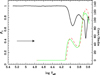 |
Fig. 1. DA-type white dwarf models (1.0 M⊙). The thick solid line represents the GDE as a function of effective temperature. The continuous thin line indicates the ratio Fc(τ)/Fr(τ) for log g = 8.5 and the dashed one denotes the same but for log g = 8.0. All calculations were performed at τ = 100.0. We note that the Teff range of the atmosphere models by Cukanovaite (in prep.) is limited to Teff ≤ 60 000 K. The arrow indicates the direction of time evolution. |
We can use Eq. (7) to help us visualise the behaviour of β1 and its relation to opacity. The connection between β1 and the convective contribution to the flux is evident; it is especially clear near the maxima and minima. The behaviour of the GDE shown in Fig. 1 (also that of the following figures) is the result of the combination of the different sources of opacity but we can gain some insight into its influence on the GDE by adopting some opacity laws in their parameterised form. Firstly, we analyse the effects of opacity in the colder models. For this range of effective temperatures one of the predominant sources of opacity is the negative hydrogen ion whose dependence on ρ and T is given by κ ≈ κ1ρ1/2T7.7, where κ1 is a constant. We note the high dependence of negative hydrogen ion opacity with temperature. The expression  in Eq. (7) drives the behaviour of the gravity-darkening exponent, and, introducing the relevant values of n and s for such models at a given convective efficiency, we get β1 ≈ 0.30. In addition, the opacities ff, bf, and bb, because of electronic transitions, are given by Kramers law: κ ≈ κ2ρT−7/2, where κ2 is a constant. The approximate corresponding value of β1 in this case is ≈0.35. Considering that Eq. (7) is just a rough approximation, these results are surprising because they predict deviations from the von Zeipel’s theorem and, in addition, they are in reasonable agreement with the values of β1 found in the literature for late-type stars (semi-empirical and theoretical ones; see below). On the other hand, one of the main sources of continuum opacity in hot star atmospheres is the so-called Thomson scattering. As known, this opacity is ‘grey’ because there is no dependence on temperature and density and it can be written as follows for the case of complete ionisation: κ ≈ 0.2(1.0 + X), where X is the hydrogen content. Using the same treatment as for the negative hydrogen ion case and Kramers law, we obtain β1 ≈ 1.00, which is in good agreement with the predictions of the von Zeipel’s theorem for hot stars. Again it is gratifying that Eq. (7) is capable of predicting the typical values of β1, even considering its limitations.
In addition to the analysis of the influence of convective flux on β1, there are other ways to correlate β1 with some physical magnitudes. Considering the additive properties of the specific entropy in the nonrelativistic case we have
![Mathematical equation: $$ \begin{aligned} {s} = B+ {N_ok\over {\mu _i}}{\ln }{T^{3/2}\over {\rho }} + {{N_ok\over {\mu _{\rm e}}}} \left[ {5\over {3}} {F_{3/2}(\alpha )\over {F_{1/2}(\alpha )}} + \alpha \right] + {4a\over {3}} {T^3\over {\rho }} , \end{aligned} $$](/articles/aa/full_html/2021/04/aa40489-21/aa40489-21-eq12.gif) (9)
(9)
where the symbols have the following meaning: B is a constant, α the degeneracy parameter, No is Avogadro’s number, k the Boltzmann constant, μi the mean molecular weight per ion, and μe is the mean molecular weight per electron. The functions F1/2(α) and F3/2(α) are auxiliary functions that can be written as
 (10)
(10)
and
 (11)
(11)
where u = p2/(2mkT), with p being the particle momentum and m its mass. The three components in Eq. (10) above can be easily identified: the second term is the entropy due to ions, the third is connected to electrons, and the fourth to radiation. We can see in Fig. 2 how the GDE is related to the entropy for the same models and conditions shown in Fig. 1. As mentioned, the convection onset is in log Teff ≈ 4.12 (log Teff onset) where a sudden variation of the entropy is indicated by a vertical arrow. This effective temperature is in agreement with those by Tremblay (in prep.). There are three other inflexion points (also marked with vertical arrows). These four points shown in Fig. 2 indicate that the entropy varies with the effective temperature (also with log g), which in turn drives the behaviour of the GDE. The changes in β1 with entropy are not surprising. Indeed, the differential of the entropy is given by dS = cp(∇ − ∇adia), where ∇ = dlnT/dlnP and ∇adia = (dlnT/dlnP)adia. On the other hand, it can be shown that, alternatively, the convective flux Fc(τ) ∝ (∇ − ∇adia)x, where x = 3 (small convective efficiency) or x = 3/2 for large convective efficiency. Thus, under determined physical conditions, the entropy can also be used as a convective stability criterion.
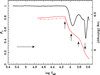 |
Fig. 2. Entropy for the same models and conditions shown in Fig. 1 (red lines). The vertical arrows indicate the points where there is a marked variation of the entropy with effective temperature. The solid line represents the entropy for τ = 100 while the dashed-dotted line denotes τ = 500; both for log g = 8.5. The horizontal arrow indicates the direction of time evolution. |
Another point to note is that the entropy does not significantly depend on the optical depth for effective temperatures ≤Teff onset. Indeed, the curves for τ = 100.0 and 500.0 coincide for Teff ≤ Teff onset. This implies that the behaviour of the resulting GDEs should not vary significantly, at least within the range of optical depths, log g, and effective temperatures explored here. We note that, for hot models, because the entropy hardly varies with Teff, the corresponding GDE values are almost constant and equal to 1.0, which restores von Zeipel’s theorem. These results are more general than those obtained decades ago, whose GDE value was constant and approximately equal to 0.32 for envelopes in convective equilibrium.
Figure 3 shows a comparison between the GDE for DB and DA models at τ = 100.0. The profiles of β1 are very similar, with the exception of the transition zone where there is a shift due to the difference in the chemical composition of the models and its influence on pressure and temperature.
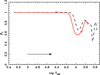 |
Fig. 3. Comparison between the GDE for a DB model (solid line, 1.0 M⊙) and DA (dashed line, 0.5 M⊙). All calculations were performed at τ = 100.0. The horizontal arrow indicates the direction of time evolution. |
An interesting comparison that can be made is related to the masses of white dwarfs. In Fig. 4 we show the evolution of the GDE for DA models with masses 1 M⊙ (continuous line) and 0.52 M⊙ (dashed line). The calculations were also performed for τ = 100.0. Because of the dependence of the onset of convection on the local gravity, the GDEs for the model with 0.52 M⊙ are shifted towards lower temperatures, in reasonable agreement with other studies (Cunningham et al. 2019, Tremblay, in prep.).
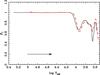 |
Fig. 4. Effect of log g on the onset of convection for DA models. The continuous line represents a sequence of DA model (1.0 M⊙) while the dashed one also denotes DA models but with 0.52 M⊙. The horizontal arrow indicates the direction of time evolution. |
As indicated, another set of evolutionary models was generated with the MESA module with an initial mass of 2.0 M⊙, X = 0.703, and Y = 0.277. For stars with convective envelopes, we employed the standard mixing-length formalism (Böhm-Vitense 1958) with αMLT = 1.80. The opacity tables adopted are those given by Grevesse & Sauval (1998). The models were followed from the PMS up to the cooling white dwarf stage. Figure 5 shows the complete evolutionary track in the HR diagram. The final mass in the cooling stage is 0.56 M⊙. The results concerning gravity-darkening are shown in Fig. 6 where we add the profile of β1 shown in Fig. 1 for comparison. Within our present level of approximation, the differences are small, being more appreciable only in the interval around log Teff ≈ 3.90.
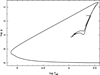 |
Fig. 5. HR diagram for an initial mass of 2.0 M⊙ from the PMS to cooling white dwarf stage. Initial chemical composition X = 0.703, Y = 0.277, αMLT = 1.80. |
As we can see in Figs. 1–4 and 6, there are clear indications of deviations from the approach by von Zeipel (1924). Deviations from von Zeipel’s theorem were previously found using suitable evolutionary models in stars evolving towards the branch of red giants and/or in low-mass main sequence stars (low effective temperatures) where the flux is predominantly convective in their envelopes (Claret 1998, 2000). Additional evidence for deviations from von Zeipel’s theorem comes from 3D simulations of cold stars (Ludwig et al. 1999). A more complete historical review about this subject can be found in above references.
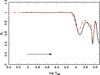 |
Fig. 6. GDE for the white dwarf cooling sequence for the models shown Fig. 5 (continuous line). The DA model shown in Fig. 1 is represented by a dashed line. The horizontal arrow indicates the direction of time evolution. |
On the other hand, there is an analytical approach by which we can explore the behaviour of GDEs in compact stars whose outermost layers are in radiative equilibrium. Such an analysis was carried out in Claret (2012) for main sequence stars. Here we adapt the physical conditions for the case of white dwarfs. Such an equation can be written as (see Appendix A)
![Mathematical equation: $$ \begin{aligned} \beta _1 \approx 1 + \left[{{2+N}-\chi (4+N)\over {2+N}} - {{2+N+\chi (-4+8\alpha _1-5N)}\over {2+N+\chi (\kappa _{\rho }-\kappa _T)(N-2\alpha _1)}}\right]{\tau _{\rm p}\over {\tau _{\rm e}}}. \end{aligned} $$](/articles/aa/full_html/2021/04/aa40489-21/aa40489-21-eq15.gif) (12)
(12)
Equation (12) opens up some possibilities on the investigation of the distribution of rotational velocities through the parameter α1 and on geometry through N. We note that this equation is valid only for hot stars. We note that the ratio τp/τe ≤ 1.0. For example, we would restore the predictions of von Zeipel’s theorem for the cases α1 = N/2 or for uniform rotation and no θ dependence. An interesting feature of Eq. (12) can be explored and is related to κρ and κT. Depending on the behaviour of these two variables, we could have values of β1 significantly smaller than 1.01. For example, for α = −1.0, N = 1, χ = 0.2, τp/τe = 0.71, and β1 = 0.80, and the resulting condition would be
![Mathematical equation: $$ \begin{aligned} -6.0 \lessapprox \left[\left({{\partial \ln \kappa }\over {\partial \ln \rho }}\right)_{T} - \left({{\partial \ln \kappa }\over {\partial \ln T}}\right)_{\rho }\right] \lessapprox -5.0. \end{aligned} $$](/articles/aa/full_html/2021/04/aa40489-21/aa40489-21-eq16.gif) (13)
(13)
Such a condition is approximately fulfilled for envelopes with effective temperatures in the interval 6000 K ⪅ Teff ⪅ 13 000 K. There are no semi-empirical data yet for white dwarfs in this effective temperature range for comparison, but it is interesting to note that values of β1 smaller than 1.0 were detected using long-baseline optical/infrared interferometry in isolated fast rotators. Some of these systems show effective temperatures within the mentioned range. A summary of their properties can be found in Table 1 of Claret (2016).
Values of the GDE smaller than 1.0 were also observationally detected in main sequence and/or subgiants stars in binary systems. However, a direct connection between the results from long-baseline interferometry and from eclipsing binaries (mostly main sequence stars) and those provided by Eq. (12) (compact ones) is not straightforward. However, it can give us some clue for future research. A turning point concerning semi-empirical β1 was the pioneering paper by Rafert & Twigg (1980) using eclipsing binaries. Such research was followed by others, such as Pantazis & Niarchos (1998), Niarchos (2000), and Djurasevic et al. (2003, 2006), for example, who explored a wide range of effective temperatures. The semi-empirical GDEs derived by these latter authors for hot stars are scattered around the classical von Zeipel value. Some of these systems show β1 as low as 0.60. Another important result of these investigations is that the derived values for systems with cooler components also contradict the predictions of von Zeipel’s theorem. These semi-empirical GDE values are quite significant but do not yet constitute a critical test of the theory of temperature distribution on a distorted stellar surface. However, despite the fact that these observations are not conclusive, they seem to indicate a transition zone for the GDE. That zone approximately coincides with the change in the prevalence of the process of energy transport in the envelopes, that is, radiative to convective, as indicated by the Fig. 3 in Claret (2003). Such a transition zone is also predicted in the present paper for compact stars.
Finally, it would be very interesting and useful if observers were to focus their attention on close binary systems constituted by white dwarfs distorted by rotation and tides, so that the validity of the preliminary calculations presented here can be verified. To constrain the GDE values observationally, it would be necessary to investigate eclipsing binary white dwarfs that are double-lined and bright enough to obtain good radial-velocity semi-amplitudes for both components. We hope that such systems will be found in the not too distant future.
We have also found significant deviations from von Zeipel’s theorem using our modified numerical method, at the upper layers of hot white dwarfs.
Acknowledgments
I would like to thank E. Cukanovaite for providing models of the structure of white dwarfs atmospheres and an anonymous referee for his/her helpful suggestions. The Spanish MEC (ESP2017-87676-C5-2-R, PID2019-107061GB-C64, and PID2019-109522GB-C52) is gratefully acknowledged for its support during the development of this work. A.C. also acknowledges financial support from the State Agency for Research of the Spanish MCIU through the “Center of Excellence Severo Ochoa” award for the Instituto de Astrofísica de Andalucía (SEV-2017-0709). This research has made use of the SIMBAD database, operated at the CDS, Strasbourg, France, and of NASA’s Astrophysics Data System Abstract Service.
References
- Althaus, L. G., Serenelli, A. M., & Benvenuto, O. G. 2001a, MNRAS, 323, 471 [NASA ADS] [CrossRef] [Google Scholar]
- Althaus, L. G., Serenelli, A. M., & Benvenuto, O. G. 2001b, MNRAS, 324, 617 [Google Scholar]
- Böhm-Vitense, E. 1958, ZAp, 46, 108 [NASA ADS] [Google Scholar]
- Burdge, K. B., Coughlin, M. W., Fuller, J., et al. 2019a, Nature, 571, 528 [Google Scholar]
- Burdge, K., Fuller, J., Phinney, E. S., et al. 2019b, ApJ, 886, L12 [Google Scholar]
- Burdge, K. B., Prince, T. A., Fuller, J., et al. 2020, ApJ, 905, 32 [Google Scholar]
- Claret, A. 1998, A&AS, 131, 395 [NASA ADS] [CrossRef] [EDP Sciences] [Google Scholar]
- Claret, A. 2000, A&A, 359, 289 [NASA ADS] [Google Scholar]
- Claret, A. 2003, A&A, 406, 623 [NASA ADS] [CrossRef] [EDP Sciences] [Google Scholar]
- Claret, A. 2012, A&A, 538, A3 [NASA ADS] [CrossRef] [EDP Sciences] [Google Scholar]
- Claret, A. 2016, A&A, 588, A15 [NASA ADS] [CrossRef] [EDP Sciences] [Google Scholar]
- Claret, A., & Bloemen, S. 2011, A&A, 529, A75 [NASA ADS] [CrossRef] [EDP Sciences] [Google Scholar]
- Claret, A., Cukanovaite, E., Burdge, K., et al. 2020, A&A, 634, A93 [EDP Sciences] [Google Scholar]
- Cukanovaite, E., Tremblay, P.-E., Freytag, B., et al. 2019, MNRAS, 490, 1010 [Google Scholar]
- Cunningham, T., Tremblay, P.-E., Freytag, B., et al. 2019, MNRAS, 488, 2503 [Google Scholar]
- Djurasevic, G., Rovithis-Livaniou, H., Rovithis, P., et al. 2003, A&A, 402, 667 [NASA ADS] [CrossRef] [EDP Sciences] [Google Scholar]
- Djurasevic, G., Rovithis-Livaniou, H., Rovithis, P., et al. 2006, A&A, 445, 291 [NASA ADS] [CrossRef] [EDP Sciences] [Google Scholar]
- Espinosa Lara, F., & Rieutord, M. 2011, A&A, A130 [Google Scholar]
- Espinosa Lara, F., & Rieutord, M. 2012, A&A, 547, A32 [NASA ADS] [CrossRef] [EDP Sciences] [Google Scholar]
- Grevesse, N., & Sauval, A. J. 1998, Space Sci. Rev., 85, 161 [Google Scholar]
- Kippenhahn, R. 1977, A&A, 58, 267 [NASA ADS] [Google Scholar]
- Kippenhahn, R., Weigert, A., & Hofmeister, E. 1967, Computational Physics (New York: Academic Press), 7, 129 [Google Scholar]
- Kopal, Z. 1959, Close Binary Systems (Chapman& Hall) [Google Scholar]
- Kupfer, T., Bauer, E. B., Burdge, K. B., et al. 2020, ApJ, 898, L25 [Google Scholar]
- Ludwig, H.-G., Freytag, B., & Steffen, M. 1999, A&A, 346, 111 [Google Scholar]
- McGill, M. A., Sigut, T. A. A., & Jones, C. E. 2013, ApJS, 204, 2 [Google Scholar]
- Niarchos, P. G. 2000, in Variable Stars as Essential Astrophysical Tools, ed. C. Ibanoglu, 544, 631 [Google Scholar]
- Pantazis, G., & Niarchos, P. G. 1998, A&A, 335, 199 [NASA ADS] [Google Scholar]
- Paxton, B., Bildsten, L., Dotter, A., et al. 2011, ApJS, 192, 3 [Google Scholar]
- Paxton, B., Cantiello, M., Arras, P., et al. 2013, ApJS, 208, 4 [NASA ADS] [CrossRef] [Google Scholar]
- Paxton, B., Marchant, P., Schwab, J., et al. 2015, ApJS, 220, 15 [Google Scholar]
- Rafert, J. B., & Twigg, L. W. 1980, MNRAS, 193, 79 [Google Scholar]
- Renedo, I., Althaus, L. G., Miller Bertolami, M. M., et al. 2010, ApJ, 717, 183 [NASA ADS] [CrossRef] [Google Scholar]
- von Zeipel, H. 1924, MNRAS, 84, 665 [Google Scholar]
Appendix A: Brief description of the derivation of Eq. (12)
For completeness, we give here a brief summary of the derivation of Eq. (12) which is a generalisation of von Zeipel’s theorem. For more details, see Kippenhahn (1977) and Claret (2012).
Let us assume that the angular velocity has the following general form
 (A.1)
(A.1)
where h(r) is a generic function and θ is the colatitude angle. In our approach we assume that the effect of the centrifugal force on the stellar structure is small. The total potential ψ can be written as
 (A.2)
(A.2)
The integrating factor was chosen in such a way that Λg can be derived from a potential. As a consequence, it can be shown that the pressure is constant on equipotential surfaces. If the effects of rotation are small, we obtain for the integrating factor:
 (A.3)
(A.3)
In the above equation we define  and χ = r3ω2/(GMψ).
On the other hand, the equation of the radiative transport can be written as
 (A.4)
(A.4)
Assuming that the density and temperature are functions of the structural form of the potential we have ρ = d(Ψ)Λ and T = t(Ψ)/Λ and
 (A.5)
(A.5)
As an extra condition we adopt the relationship g(μe)τ(μe, ψ) = g(μp)τ(μp, ψ), where the subscripts e and p denote values at the equator and at the poles. Calculating the values of local gravity, of Λ and of Eq. (A.5) at the pole and at the equator we finally obtain the GDE through the logarithmic derivatives of the flux and effective gravity
 (A.6)
(A.6)
After some algebra and incorporating the effects of variable opacity we finally get
![Mathematical equation: $$ \begin{aligned}&\beta _1 \approx 1 +\left[{{2+N}-\chi (4+N)\over {2+N}}- {{2+N+\chi (-4+8\alpha _1-5N)}\over {2+N+\chi (\kappa _{\rho }-\kappa _T)(N-2\alpha _1)}}\right] \nonumber \\&{\tau _{\rm p}\over {\tau _{\rm e}}} , \end{aligned} $$](/articles/aa/full_html/2021/04/aa40489-21/aa40489-21-eq24.gif) (A.7)
(A.7)
where  and
and  .
.
All Figures
|
Fig. 1. DA-type white dwarf models (1.0 M⊙). The thick solid line represents the GDE as a function of effective temperature. The continuous thin line indicates the ratio Fc(τ)/Fr(τ) for log g = 8.5 and the dashed one denotes the same but for log g = 8.0. All calculations were performed at τ = 100.0. We note that the Teff range of the atmosphere models by Cukanovaite (in prep.) is limited to Teff ≤ 60 000 K. The arrow indicates the direction of time evolution. |
| In the text | |
|
Fig. 2. Entropy for the same models and conditions shown in Fig. 1 (red lines). The vertical arrows indicate the points where there is a marked variation of the entropy with effective temperature. The solid line represents the entropy for τ = 100 while the dashed-dotted line denotes τ = 500; both for log g = 8.5. The horizontal arrow indicates the direction of time evolution. |
| In the text | |
|
Fig. 3. Comparison between the GDE for a DB model (solid line, 1.0 M⊙) and DA (dashed line, 0.5 M⊙). All calculations were performed at τ = 100.0. The horizontal arrow indicates the direction of time evolution. |
| In the text | |
|
Fig. 4. Effect of log g on the onset of convection for DA models. The continuous line represents a sequence of DA model (1.0 M⊙) while the dashed one also denotes DA models but with 0.52 M⊙. The horizontal arrow indicates the direction of time evolution. |
| In the text | |
|
Fig. 5. HR diagram for an initial mass of 2.0 M⊙ from the PMS to cooling white dwarf stage. Initial chemical composition X = 0.703, Y = 0.277, αMLT = 1.80. |
| In the text | |
|
Fig. 6. GDE for the white dwarf cooling sequence for the models shown Fig. 5 (continuous line). The DA model shown in Fig. 1 is represented by a dashed line. The horizontal arrow indicates the direction of time evolution. |
| In the text | |
Current usage metrics show cumulative count of Article Views (full-text article views including HTML views, PDF and ePub downloads, according to the available data) and Abstracts Views on Vision4Press platform.
Data correspond to usage on the plateform after 2015. The current usage metrics is available 48-96 hours after online publication and is updated daily on week days.
Initial download of the metrics may take a while.