© ESO 2021

1. Introduction

The kinetics of inertial particles that are (finite-size particles that are massive enough to have significant inertia) in turbulence has drawn much attentions for decades. It has been driven by wide applications in astrophysics, atmospheric sciences, and engineering. The preferential concentration and fractal clustering of inertial particles in (nearly) incompressible turbulence has been simulated extensively (see Maxey 1987; Squires & Eaton 1991; Eaton & Fessler 1994; Bec 2003, 2005; Bec et al. 2007a,b; Bhatnagar et al. 2018; Yavuz et al. 2018). In combination with the theory of coagulation of particles, this has an important application in planet-formation theory (see e.g. Pan et al. 2011; Birnstiel et al. 2016; Johansen et al. 2012; Johansen & Lambrechts 2017). However, proto-planetary discs are dominated by low Mach-number turbulence, which is not the case in many other astrophysical environments. One example is the cold phase of the interstellar medium (ISM), where turbulence is highly compressible with Mach numbers of order 10 and thus is dominated by shock waves. Only a few studies of inertial particles in high Mach-number turbulence can be found in the literature (e.g. Hopkins & Lee 2016; Mattsson et al. 2019a,b), and direct numerical simulations of turbulence-driven coagulation of inertial particles have not been performed so far. Exploring the effects of compressibility (high Mach numbers) on coagulation is therefore an important branch of research that is now becoming possible through the rapid development of computing power.

From an astrophysical perspective, cosmic dust grains, which are made of mineral or carbonaceous material and are a perfect example of inertial particles, are ubiquitous throughout the universe. Rapid interstellar dust growth by accretion of molecules is thought to be necessary to compensate for various dust destruction processes (see e.g. Mattsson 2011; Valiante et al. 2011; Rowlands et al. 2014). Grains may also grow by aggregation or coagulation (which does not increase the dust mass), however, when the growth by accretion has produced large enough grains for coagulation to become efficient, that is, once the ‘coagulation bottleneck’ has been passed (Mattsson 2016). How efficient the coagulation is in molecular clouds (MCs) is not fully understood, although models and simulations have suggested that turbulence is the key to high growth efficiency (Elmegreen & Scalo 2004; Hirashita & Yan 2009; Hirashita 2010; Pan et al. 2014a,b; Pan & Padoan 2015; Hopkins & Lee 2016; Mattsson et al. 2019a,b) and observations indicate the presence of very large grains (which can be tens of μm across) in the cores of MCs (Hirashita et al. 2014).

We aim to study the role that the Mach number plays for the coagulation of inertial particles in compressible turbulence. Specifically, we strive to study how coagulation of particles depends on Mach number in regions where the particles cluster and form filaments. The purpose is not to target any specific astrophysical context, but to explore the Mach-number dependence to the extent that this is computationally feasible. There are three main challenges. First, the dynamics of inertial particles in compressible turbulence is poorly understood. Second, the coagulation process is a non-equilibrium process, as the particle size distribution evolves with time. Third, the coagulation timescale and the characteristic timescale of the turbulence are very different in dilute systems, such as those typically studied in astrophysics. In classical kinetic theory, the collision kernel C_ij is a function of the relative velocity Δv_ij of two particles i and j, which is difficult to calculate analytically, except in some special cases. For the same reason, it is difficult to calculate the coagulation rate using analytical models. More exactly, the classical Smoluchowski (1916) problem has only three known exact solutions (Aldous 1999), and numerical solution of the coagulation equation is only feasible if treated as a local or ‘zero-dimensional’ problem.

The main objective of the present work is to offer a way to quantify and possibly parametrise the effects of turbulent gas dynamics and hydrodynamic drag on the coagulation rate in such a way that it can be included for instance in traditional models of galactic chemical evolution (including dust), which are based on average physical quantities (Mattsson 2016). A major problem when simulating the dust growth in the ISM is that the system is large scale and dilute. The coagulation rate is extremely low in such a system, which leads to very different timescales for the turbulent gas dynamics and coagulation.

2. Turbulence and kinetic drag

In this section, equations governing compressible flow and particle dynamics of inertial particles (e.g. dust grains) are presented. The PENCIL CODE with HDF5 IO (Brandenburg et al. 2021; Bourdin 2020) is used to solve these equations.

Since the carrier fluid in our study is isothermal, its turbulence described by Eq. (1) is scale free, that is, the box size L, the mean mass density ⟨ρ⟩, and the sound speed c_s are the unit length, unit density, and unit velocity, respectively. These quantities can thus be scaled freely. However, the inclusion of coagulation process means our simulation is no longer scale free. This requires a careful treatment of initial conditions and scaling of units, which is discussed in more detail in Sect. 3.4.

2.1. Momentum equation of the carrier flow

The motion of the gas flow is governed by the Navier-Stokes equation,

$$\begin{array}{c}\hfill \frac{\partial \mathit{u}}{\partial t}+\mathit{u}·\mathbf{\nabla }\mathit{u}=\mathit{f}-{\rho }^{-1}\mathbf{\nabla }p+{\rho }^{-1}{\mathit{F}}_{\mathrm{visc}},\end{array}$$(1)

where f is a forcing function (Brandenburg 2001), p is the gas pressure, and ρ is the fluid or gas density obeying the continuity equation,

$$\begin{array}{c}\hfill \frac{\partial \rho }{\partial t}+\mathbf{\nabla }·(\rho \mathit{u})=0.\end{array}$$(2)

For the case of direct numerical simulation with a constant kinetic viscosity of the gas flow, the viscosity term F_visc equals the physical viscosity term ${\mathit{F}}_{\mathrm{visc}}^{\nu }$ given by

$$\begin{array}{c}\hfill {\mathit{F}}_{\mathrm{visc}}^{\nu }=\rho \nu ({\mathbf{\nabla }}^2\mathit{u}+\frac{1}{3}\mathrm{\nabla }\mathrm{\nabla }·\mathit{u}+2\mathit{S}·\mathrm{\nabla }ln\rho ),\end{array}$$(3)

where $\mathit{S}=\frac{1}{2}[\mathbf{\nabla }\mathit{u}+{\left(\mathbf{\nabla }\mathit{u}\right)}^T]-\frac{1}{3}(\mathbf{\nabla }·\mathit{u})\mathsf{I}$ is the rate-of-strain tensor (I is the unit tensor) resulting from the shear effect and the deformation due to compression. For the case with shock-capturing viscosity, the viscosity term becomes

$$\begin{array}{c}\hfill {\mathit{F}}_{\mathrm{visc}}={\mathit{F}}_{\mathrm{visc}}^{\nu }+\rho {\zeta }_{\mathrm{shock}}\mathrm{\nabla }\mathrm{\nabla }·\mathit{u}+(\mathrm{\nabla }·\mathit{u})\mathrm{\nabla }\left(\rho {\zeta }_{\mathrm{shock}}\right).\end{array}$$(4)

The shock viscosity ζ_shock is given by

$$\begin{array}{c}\hfill {\zeta }_{\mathrm{shock}}=c_{\mathrm{shock}}⟨\max [{(-\mathbf{\nabla }·\mathit{u})}_{+}]⟩{(min(\delta x,\delta y,\delta z))}^2,\end{array}$$(5)

where c_shock is a constant defining the strength of the shock viscosity (Haugen et al. 2004). The length of the lattice is given by δx, δy, and δz, respectively. ${\mathit{F}}_{\mathrm{visc}}^{\mathrm{shock}}$ is used in simulations with high Mach number, where we strive to use the highest spatial resolution to capture the shocks. Nevertheless, it is necessary to introduce this term to handle the strongest shocks. Two dimensionless parameters characterise compressible turbulence: the Reynolds number Re and the root-mean-square (rms) Mach number ℳ_rms. Re is defined as

$$\begin{array}{c}\hfill \mathrm{Re}\equiv u_{\mathrm{rms}}{L}_{\mathrm{inj}}/\nu ,\end{array}$$(6)

where u_rms is the rms turbulent velocity and L_inj is the energy injection length scale. The compressibility of the flow is characterised by ℳ_rms, which is defined as

$$\begin{array}{c}\hfill {\mathcal{M}}_{\mathrm{rms}}=u_{\mathrm{rms}}/c_{\mathrm{s}},\end{array}$$(7)

where c_s is the sound speed. The sound speed is kept constant because the compressible flow to be investigated here is assumed to be isothermal such that $c_{\text{s}}^2=\gamma p/\rho$, where γ = c_P/c_v = 1 with the specific heats c_P and c_V at constant pressure and constant volume, respectively. Another quantity is the mean energy dissipation rate $⟨\overline{ϵ}⟩$, which measures how vigorous the small eddies are in turbulence. It can be calculated from the trace of S_ij as $⟨\overline{ϵ}⟩=2\nu \overline{\mathrm{Tr}{\mathsf{S}}_{\mathsf{ij}}{\mathsf{S}}_{\mathsf{ji}}}$. $⟨\overline{ϵ}⟩$ determines the smallest scales of the turbulence, for example, the Kolmogorov length scale is defined as $\eta ={({\nu }^3/⟨\overline{ϵ}⟩)}^{1/4}$ and the timescale is defined as ${\tau }_{\eta }={(\nu /⟨\overline{ϵ}⟩)}^{1/2}$. Becausee the Saffman-Turner collision rate is proportional to ${\tau }_{\eta }^{-1}$ (Saffman & Turner 1956), $⟨\overline{ϵ}⟩$ indirectly determines the coagulation rate of particles in an incompressible flow. Coagulation occurs at the small scales of turbulence, and the strength of the small eddies determines the particle velocity (Li et al. 2018). Therefore it is worth investigating whether and how $⟨\overline{ϵ}⟩$ affects the coagulation rate in compressible turbulence as well. We show that it does not affect the coagulation rate in the compressible case.

The stochastic solenoidal forcing f is given by

$$\begin{array}{c}\hfill \mathit{f}(\mathit{x},t)=\mathrm{Re}\{N{\mathit{f}}_{\mathit{k}(t)}exp[i\mathit{k}(t)·\mathit{x}+i\varphi (t)]\},\end{array}$$(8)

where k(t) is the wave space, x is position, and ϕ(t) (|ϕ|< π) is a random phase. The normalization factor is given by N = f₀c_s(kc_s/Δt)^1/2, where f₀ is a non-dimensional factor, k = |k|, and Δt is the integration time step (Brandenburg & Dobler 2002). We chose a completely non-helical forcing, that is,

$$\begin{array}{c}\hfill {\mathit{f}}_{\mathit{k}}=(\mathit{k}\times \mathit{e})/\sqrt{{\mathit{k}}^2-{(\mathit{k}·\mathit{e})}^2},\end{array}$$(9)

where e is the unit vector.

To achieve different ℳ_rms with fixed Re and $⟨\overline{ϵ}⟩$ in the simulations, we need to change u_rms, ν, and the simulation box L simultaneously according to Eqs. (6) and (7), and we also considered

$$\begin{array}{c}\hfill ⟨\overline{ϵ}⟩\sim \frac{u_{\mathrm{rms}}^3}{L_{\mathrm{inj}}}.\end{array}$$(10)

Since u_rms is essentially determined by the amplitude of forcing f₀, we changed f₀ in the simulation as well.

2.2. Particle dynamics

The trajectories of inertial particles is determined by

$$\begin{array}{c}\hfill \frac{\mathrm{d}{\mathit{x}}_i}{\mathrm{d}t}={\mathit{v}}_i\end{array}$$(11)

and

$$\begin{array}{c}\hfill \frac{\mathrm{d}{\mathit{v}}_i}{\mathrm{d}t}=\frac{1}{{\tau }_i}(\mathit{u}-{\mathit{v}}_i),\end{array}$$(12)

where

$$\begin{array}{c}\hfill {\tau }_i=\sqrt{\frac{\pi }{8}}\frac{{\rho }_{\mathrm{mat}}}{\rho }\frac{a}{c_{\mathrm{s}}}{(1+\frac{9\pi }{128}\frac{|\mathit{u}-{\mathit{v}}_i{|}^2}{c_{\mathrm{s}}^2})}^{-1/2},\end{array}$$(13)

is the stopping time, that is, the kinetic-drag timescale. In the equation above, a is the radius of a particle, ρ_mat is the material density of particles, and ρ is the mass density of the gas. We assumed that particles are well described in the Epstein limit because the mean-free-path λ is large and particles are small in most astrophysical contexts (large Knudsen number, Kn =λ/a ≫ 1; Armitage 2010). The stopping time at low relative Mach number (𝒲 = |u − v_i|/c_s ≪ 1) is

$$\begin{array}{c}\hfill {\tau }_i(\mathcal{W}\ll 1)=\sqrt{\frac{\pi }{8}}\frac{{\rho }_{\mathrm{mat}}}{\rho }\frac{a}{c_{\mathrm{s}}}.\end{array}$$(14)

The term in parentheses of Eq. (13) is a correction for high 𝒲. Equation (13) is essentially a quadratic interpolation between the two expressions for the limits 𝒲 ≪ 1 and 𝒲 ≫ 1 derived from the exact expression for τ_i (see Schaaf 1963; Kwok 1975; Draine & Salpeter 1979).

To characterize the inertia of particles, we define a ‘grain-size parameter’ as

$$\begin{array}{c}\hfill \alpha =\frac{{\rho }_{\mathrm{mat}}}{⟨\rho ⟩}\frac{a}{L},\end{array}$$(15)

which is the parametrisation used by Hopkins & Lee (2016). Because the total mass of a simulation box of size L, as well as the mass of a grain of a given radius a, is constant, the quantity α is solely determined by a regardless of the characteristics of the simulated flow.

In general, the inertia of particles is characterised by the Stokes number St = τ_i/τ_η. The disadvantage of St as the size parameter for inertial particles in a highly compressible carrier fluid is that a fluid flow with Re ≫ 1 cannot be regarded as a Stokes flow. If ℳ_rms ≫ 1 as well, St is not even well defined as an average quantity in a finite simulation domain. The parameter α is therefore a better dimensionless measure of grain size than the average Stokes number ⟨St⟩ for a supersonic compressible flow. Moreover, ⟨St⟩ is not only a function of the size, but also a function of the mean energy dissipation rate $⟨\overline{ϵ}⟩$, which complicates the picture even further.

2.3. Averages

In the following we frequently refer to the mean or average quantities of three different types. For each of them we use a different notation. First, we use the bracket notation ⟨Q⟩ for volume averages, taken over the whole simulation box unless stated otherwise. Second, we use the over-bar notion $\overline{Q}$ for straight time-averaged quantities. Third, we use the tilde notation $\stackrel{\sim }{Q}$ for ensemble averages, that is, averages defined by the first moment of the distribution function of the particles.

The rms value of a fluctuating physical quantity has been mentioned in Sect. 1. In terms of the above notion, rms values always refer to $Q_{\mathrm{rms}}\equiv \sqrt{⟨Q^2⟩}$.

3. Coagulation

3.1. Numerical treatment of coagulation

The most physically consistent way to model coagulation is to track each individual Lagrangian particle and to measure the collisions among them when they overlap in space, which is computationally challenging because the coagulation timescale of inertial particles is often much shorter than the Kolmogorov timescale. We also used 10⁷ representative particles, which means solving a large N-body problem. Because of the aforementioned computational load, a super-particle approach is often used to study the coagulation of dust grains (Zsom & Dullemond 2008; Johansen et al. 2012; Li et al. 2017). Instead of tracking each individual particles, super-particles consisting of several identical particles are followed. Within each super-particle, all the particles have the same velocity v_i and size a. The super-particle approach is a Monte Carlo approach, which treats coagulation of dust grains in a stochastic manner (Bird 1978, 1981; Jorgensen et al. 1983). Each super-particle is assigned a virtual volume that is the same as the volume of the lattice, therefore a number density n_j.

When two super-particles i and j reside in the same grid cell, the probability of coagulation is $p_{\mathrm{c}}={\tau }_{\mathrm{c}}^{-1}\mathrm{\Delta }t$, where τ_c is the coagulation time and Δt is the integration time step. A coagulation event occurs when p_c > η_c, where η_c is a random number. The coagulation timescale τ_c is defined as

$$\begin{array}{c}\hfill {\tau }_{\mathrm{c}}^{-1}={\sigma }_{\mathrm{c}}{n}_j|{\mathit{w}}_{\mathit{ij}}|E_{\mathrm{c}},\end{array}$$(16)

where σ_c = π(a_i + a_j)² and w_ij are the geometric coagulation cross section and the absolute velocity difference between two particles with radii a_i and a_j, respectively, and E_c is the coagulation efficiency (Klett & Davis 1973). For simplicity, we set E_c to unity. This means that all particles coalesce upon collision, that is, bouncing and fragmentation are neglected. This treatment may overestimate the collision rate but does not affect the dynamics of particles. Therefore the ℳ dependence should not be affected. Compared with the super-particle algorithm that is widely used in planet formation (Zsom & Dullemond 2008; Johansen et al. 2012), our algorithm provides better collision statistics (Li et al. 2017). We refer to Li et al. (2017) for a detailed comparison of the super-particle algorithm used in Johansen et al. (2012) and Li et al. (2017, 2018, 2020).

3.2. Timescale differences

Before we describe the basic theory of coagulation of particles in a turbulent carrier fluid, it is important that we consider the different timescales that are involved in this complex and composite problem. In Eq. (16), we introduced τ_c. The other important timescale in a model of coagulation of particles in turbulence is the flow timescale of the carrier fluid, in this case, the large-eddy turnover time τ_L = L/u_rms, where u_rms is the rms flow velocity. Clearly, τ_L depends on the scaling of the simulation. When we compare the two timescales, we find that

$$\begin{array}{c}\hfill \frac{{\tau }_L}{⟨{\tau }_{\mathrm{c}}⟩}\sim N_{\mathrm{p}}\frac{a^2}{L^2}\frac{⟨|{\mathit{w}}_{\mathit{ij}}|⟩}{u_{\mathrm{rms}}},\end{array}$$(17)

where N_p is the total number of particles in the simulated volume. We note that ⟨|w_ij|⟩/u_rms ≪ 1 as long as the particles do not decouple completely from the carrier flow. In order to avoid slowing down the simulation too much, we aim for τ_L/⟨τ_c⟩∼1. From this we may conclude that N_p ≫ (L/a)², which implies that if we have an upper bound of N_p for computational reasons, we cannot simulate tiny particles in a large volume. The ratio τ_L/⟨τ_c⟩ shows how difficult it can be to simulate the coagulation in astrophysical contexts, in particular when the details of coagulation of inertial particles are simulated in a carrier fluid representing well-resolved compressible turbulence.

In addition to the two timescales discussed above, we must also consider the stopping time τ_i of the particles because we study inertial particles. For α ≲ 0.1, τ_i is typically smaller than τ_L. Hence, the competing timescales would rather be τ_c and τ_i, which suggests that the ratio τ_i/τ_c should be of order unity to avoid slowing down the simulation compared to the case of non-interacting particles. By the same assumptions as above (k_f ≈ 3 and E_c ∼ 1), we can show that

$$\begin{array}{c}\hfill \frac{{\tau }_i}{⟨{\tau }_{\mathrm{c}}⟩}\sim \frac{⟨|{\mathit{w}}_{\mathit{ij}}|⟩}{c_{\mathrm{s}}}\frac{{\rho }_{\mathrm{p}}}{\rho }{a}_i^3,\end{array}$$(18)

where ρ_p≡ρ_mat n_i is the mass density of particles (not to be confused with the bulk material density ρ_mat). In many astrophysical contexts (in particular, cold environments) ⟨|w_ij|⟩/c_s ∼ 1, which then suggests we must have ρ_p/ρ ∼ 1. This is always inconsistent with cosmic dust abundances, however, whether in stars, interstellar clouds, or even proto-planetary discs. In the cold ISM, ρ_p/ρ ∼ 10⁻² and ⟨|w_ij|⟩/c_s ∼ 1, which implies that τ_i/τ_c ≪ 1 and thus the time step of a simulation of coagulation in such an environment is limited by τ_i. In practice, this means that it will be difficult (or even impossible) to target coagulation in cold molecular clouds in the ISM without highly specialised numerical methods.

The goal of the present study is primarily to investigate how coagulation of inertial particles depends on ℳ_rms and not to simulate coagulation in a realistic and dilute astrophysical environment. We note, however, that any result on coagulation of particles in compressible turbulence is primarily of importance for astrophysics, for instance, the processing of dust grains in the ISM and various types of circumstellar environments. Therefore we tried to make the simulation system as dilute, while still ensuring statistical convergence and computational feasibility.

3.3. Theory of coagulation of inertial particles in turbulence

Coagulation, as described by the Smoluchowski (1916) equation, is determined by the coagulation rate R_ij between two grains species (sizes) i and j and the associated rates of depletion. In general, we have $R_{\mathit{ij}}=\frac{1}{2}{n}_i{n}_j{C}_{\mathit{ij}}$, where n_i, n_j are the number densities of the grains i and j, and C_ij is the collision kernel. Turbulence has been proposed to have a profound effect on C_ij, and we focus this theory section on what happens to C_ij.

Assuming the distribution of particle pairs can be separated into distinct spatial and velocity distributions, we have (Sundaram & Collins 1997)

$$\begin{array}{c}\hfill ⟨C_{\mathit{ij}}⟩=\pi {(a_i+a_j)}^{2}g(r,a_i,a_j){\displaystyle \int }{\mathit{w}}_{\mathit{ij}}P({\mathit{w}}_{\mathit{ij}},a_i,a_j)\mathrm{d}{\mathit{w}}_{\mathit{ij}},\end{array}$$(19)

where g is the radial distribution function (RDF) and P is the probability density distribution of relative velocities w_ij.

Below, we review the basic theory of coagulation in the tracer particle limit and large-inertial limit. Since small-clustering is negligible for both small- and large-inertial particles, we implicitly assumed that g(r) = 1. Moreover, in case of Maxwellian velocities, that is, P(w_ij, a_i, a_j) follows a Maxwellian distribution, the integral part of Eq. (19) becomes $⟨{\mathit{w}}_{\mathit{ij}}⟩=\sqrt{8\pi /3⟨{\mathit{w}}_{\mathit{ij}}·{\mathit{w}}_{\mathit{ij}}⟩}$. Thus, the collision kernel in Eq. (19) reduces to

$$\begin{array}{c}\hfill ⟨C_{\mathit{ij}}⟩=\sqrt{8\pi /3}{(a_i+a_j)}^2\sqrt{⟨{\mathit{w}}_{\mathit{ij}}·{\mathit{w}}_{\mathit{ij}}⟩},\end{array}$$(20)

which is the form assumed in the two following subsections.

3.3.1. Tracer-particle limit

In the low-inertial limit, also known as the Saffman-Turner limit or the tracer-particle limit (Saffman & Turner 1956), $\langle {\mathit{w}}_{ij}^2\rangle$ is a simple function of a_i and a_j. In case of a mono-dispersed grain population (a = a_i = a_j) suspended in a turbulent low Mach-number medium, we may use the Saffman & Turner (1956) assumption, $⟨{\mathit{w}}_{\mathit{ij}}^2⟩=\frac{1}{5}{(a/{\tau }_{\eta })}^2$, where ${\tau }_{\eta }=\sqrt{\nu /⟨\overline{ϵ}⟩}$ is the Kolmogorov timescale. This is a reasonable approximation if ℳ_rms is not too large. The Saffman & Turner (1956) theory relies on w_ij having a Gaussian distribution (Maxwellian velocities) and the final expression for ⟨C_ij⟩ becomes

$$\begin{array}{c}\hfill ⟨C_i⟩=\sqrt{\frac{8\pi }{15}}\frac{{\left(2a_i\right)}^3}{{\tau }_{\eta }}.\end{array}$$(21)

For the multi-dispersed case, we replace 2a_i by (a_i + a_j) in Eq. (21).

At first sight, compressibility does not seem to play any role at all, given the collision kernel ⟨C_ij⟩ above. However, it can affect the number density of particles n_i, and therefore, R_ij. In the tracer particle limit, the spatial distribution of particles is statistically the same as for gas. Simulations have shown that the gas density of isothermal hydrodynamic turbulence exhibits a lognormal distribution (e.g. Federrath et al. 2009; Hopkins & Lee 2016; Mattsson et al. 2019a) with a standard deviation of ${\sigma }_{\rho }^2$ that is empirically related to ℳ_rms (see e.g. Passot & Vázquez-Semadeni 1998; Price et al. 2011; Federrath et al. 2010). Consequentially, n_i depends on ℳ_rms, and so does R_ij.

3.3.2. Large-inertia limit

In the opposite limit, the large-inertia limit, particles should behave according to kinetic theory. As shown by Abrahamson (1975), we have in this limit that particles are randomly positioned and follow a Maxwellian velocity distribution. In this case, we may conclude that $\langle {\mathit{w}}_{ij}^2\rangle =\langle {\mathit{v}}_i^2\rangle +\langle {\mathit{v}}_j^2\rangle$ because the particles are then statistically independent and thus they have a covariance that is identically zero. As in the tracer-particle limit, the expression for a mono-disperesed population becomes

$$\begin{array}{c}\hfill ⟨C_i⟩=a^2{\left(\frac{16\pi }{3}⟨{\mathit{v}}_i^2⟩\right)}^{1/2}.\end{array}$$(22)

Previous theoretical work on inertial particles in turbulent flows (e.g. Abrahamson 1975; Hopkins & Lee 2016; Mattsson et al. 2019a; Pan & Padoan 2013; Wang et al. 2000) have shown that the rms velocity v_rms of the particles is a function of their size. More precisely, we can parametrise in terms of grain size such that $v_{\text{rms}}^2(a_i)/u_{\text{rms}}^2\approx a_0/a_i$ for a/a₀ ≫ 1, where a₀ is a scaling radius that can be estimated from the stopping time τ_i and the integral timescale τ_L. Assuming Maxwellian velocity distributions again, we have that $\langle {\mathit{w}}_{ij}\cdot {\mathit{w}}_{ij}\rangle =v_{\text{rms}}^2(a_i)+v_{\text{rms}}^2(a_j)$. Thus, the mean collision kernel for the multi-dispersed case can be expressed as

$$\begin{array}{c}\hfill ⟨C_{\mathit{ij}}⟩\approx \sqrt{\frac{8\pi }{3}}{(a_i+a_j)}^2{u}_{\mathrm{rms}}{(\frac{a_0}{a_i}+\frac{a_0}{a_j})}^{1/2}.\end{array}$$(23)

Here, we may note that ⟨C_ij⟩ is proportional to u_rms, implying that the collision rate should scale with ℳ_rms. For particles of equal size, that is, a_i = a_j, ⟨C_ij⟩ reduces to the form given above in Eq. (22), which also means that $\langle C_i\rangle \sim a_i^{5/2}$. In the absence of external body forces other than kinetic drag, $\langle {\mathit{v}}_i^2\rangle \to 0$ for very large inertia particles. Thus, ⟨C_ij⟩→0, eventually.

To summarise, we note that for the tracer-particle limit (small-inertia particles, St ≪1), density variations in high-ℳ_rms turbulence, and the locally elevated number densities (n_i) of dust particles that follows consequently, can have a significant impact on the average collision rate ⟨R_ij⟩, although not on ⟨C_ij⟩. For particles with large inertia, beyond the effect of compressibility on ⟨R_ij⟩, caustics in the particle phase may also contribute to ⟨C_ij⟩ (see Appendix A for details of the discussion).

3.4. Initial conditions

Super-particles were initially distributed randomly in the simulation box and mono-dispersed in size (α₀ = 10⁻⁴). As discussed in Sect. 3.1, each super-particle was assigned a virtual volume (δx)³, where δx is the lateral size of the lattice. With an initial number density of dust grains n₀, the total number of dust grains in the computational domain is given by

$$\begin{array}{c}\hfill n_0{L}^3=N_{\mathrm{s}}(n_j\delta x^3),\end{array}$$(24)

where N_s is initial total number of super-particles. Since (L/δx)³ = N_grid with N_grid the number of grid cells, Eq. (24) can be rewritten as

$$\begin{array}{c}\hfill n_0{N}_{\mathrm{grid}}=N_{\mathrm{s}}{n}_j,\end{array}$$(25)

where n_j is the number density within each super-particle at t = 0. The number of physical particles in each super-particle N_p/s is determined by

$$\begin{array}{c}\hfill N_{\mathrm{p}/\mathrm{s}}=N_{\mathrm{p}}/N_{\mathrm{s}}=\frac{L^3}{N_{\mathrm{grid}}}{n}_j,\end{array}$$(26)

which means that N_p/s is uniquely determined by L³ when N_s, N_grid, and n_j are fixed.

To avoid running out of memory while executing the simulation, we must limit the number of super-particles to N_s ∼ 10⁷, which leads to a required resolution N_grid = 512³. The value of n₀ must be chosen for computational feasibility, and we also kept the number of particles within each super-particle to a minimum to avoid averaging out too much of the turbulence effects (as explained in Sect. 3.1).

We can take the physical parameters of dust grains in the ISM as an example of how difficult it is to simulate a dilute system, even on a current modern supercomputer. According to Eqs. (16) and (24), the collision frequency is proportional to n₀. With n₀ = 3.33 × 10⁻⁷ cm⁻³, a₀ = 10⁻⁶ cm, |v_i − v_j|≈10⁵ cm s⁻¹, and E_c ≈ 1, the initial collision frequency is ${\tau }_{\mathrm{c}}^{-1}\approx {10}^{-9}{\mathrm{s}}^{-1}$. The simulation time step must match the corresponding physical coagulation timescale for the particles, which is far beyond the computational power at our disposal in case of a small number of particles within each super-particle.

3.5. Diagnostics

The coagulation process is sensitive to the large-particle tail of the particle size distribution f(a, t) because particle coagulation is strongly dependent on the total cross section. The tails of f(a, t) can be characterised using the normalised moments of radius a (Li et al. 2017),

$$\begin{array}{c}\hfill a_{\zeta }={(M_{\zeta }/M_0)}^{1/\zeta },\end{array}$$(27)

where

$$\begin{array}{c}\hfill M_{\zeta }(t)={\displaystyle {\int }_0^{\infty }f(a,t)a^{\zeta }\mathrm{d}a,}\end{array}$$(28)

is the ζth moment of a. We adopted ζ = 24 to characterise the large-particle tail. To follow the overall evolution of f(a, t), we also considered the mean radius, defined by the first-order normalised moment, $\stackrel{\sim }{a}=a_1=M_1/M_0$. The relative standard deviation of f(a, t) can be defined as

$$\begin{array}{c}\hfill {\sigma }_a/\stackrel{\sim }{a}={(a_2^2-a_1^2)}^{1/2}/a_1,\end{array}$$(29)

where ${\sigma }_a={(a_2^2-a_1^2)}^{1/2}$ is the standard deviation of a.

4. Results

To investigate how coagulation depends on the Mach number ℳ_rms, we performed simulations for different ℳ_rms ranging from 0.07 to 2.58 while keeping Re and $⟨\overline{ϵ}⟩$ fixed (see the details of the simulation setup in Table 1). As shown in Fig. 1, the power spectra follow the classical Kolmogorov −5/3 law. Because the Reynolds number that can be achieved in DNS studies is much lower than the one in the ISM, large-scale separation of turbulence is not observed.

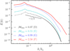Fig. 1. Power spectra for simulations of different ℳrms: ℳrms = 0.07 (solid dotted black curve), 0.55 (dashed cyan curve), 0.99 (dotted blue curve), and 2.58 (red curve). The dashed black curve shows the Kolmogorov −5/3 law.

Next, we inspected the time evolution of the dust size distribution f(a, t). As shown in Fig. 2, the tail of f(a, t) widens with increasing ℳ_rms. The broadening of f(a, t) is slowest for the nearly incompressible flow with ℳ_rms = 0.07 (solid dotted black curve). A transition is observed when the flow pattern changes from subsonic (ℳ_rms ∼ 0.5) to transonic or supersonic (ℳ_rms ≳ 1)¹, where the broadening and the extension of the tail of f(a, t) become prominent. This is further evidenced by the simulations with ℳ_rms = 0.75 (dash dotted magenta curve) and ℳ_rms = 0.99 (dotted blue curve), in the intermediate transonic regime. The supersonic case with ℳ_rms = 2.58 displays a significant broadening of the tail.

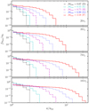Fig. 2. Time evolution of f(a, t) for simulations in Fig. 1 and for an additional simulation run H in Table 1.

Figure 3 shows the time evolution of the mean radius $\stackrel{\sim }{a}$ normalised by the initial size of particles. It is obvious that $\stackrel{\sim }{a}/a_{\mathrm{ini}}$ increases with increasing ℳ_rms. Although this does not say much about tail effects, $\stackrel{\sim }{a}$ is a good measurement of the mean evolution of f(a, t).

Fig. 3. Time evolution of $\stackrel{\sim }{a}/a_{\mathrm{ini}}$ for simulations in Fig. 2.

According to Eq. (19), the coagulation rate depends on the total cross section of the two colliding particles. Therefore growth by coagulation is sensitive to the large tail of f(a, t). As discussed in Sect. 3.5, the tail of f(a, t) can be characterised by a₂₄, that is, the 24th normalised moment. Figure 4a shows that the rate of increase of a₂₄ increases with ℳ_rms. The corresponding relative dispersion of f(a, t), ${\sigma }_a/\stackrel{\sim }{a}$, is shown in Fig. 4b, which exhibits the same ℳ_rms dependence as a₂₄. However, the form of ${\sigma }_a/\stackrel{\sim }{a}$ as a function of a₂₄/a_ini is essentially independent of ℳ_rms, as shown by the inset in Fig. 4b.

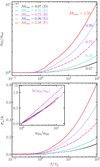Fig. 4. Time evolution of (a) the a24 and (b) ${\sigma }_a/\stackrel{\sim }{a}$ for simulations in Fig. 2. The inset shares the same y-axis as the main plot in panel b. The dashed magenta curve in the inset shows ln(a24/aini).

As mentioned in Sect. 3.3, the mean collision kernel ⟨C_ij⟩ depends on ℳ_rms. Figure 5a shows the collision kernel ⟨C_ij⟩ normalised according to ${(a_i+a_j)}_{\text{ini}}^3$, that is, the initial particle size. The Saffman-Turner model should not apply to coagulation of inertial particles in compressible turbulence as it assumes that particles act as passive tracers and are advected by the turbulent motion of the carrier. In spite of this, ⟨C_ij⟩ appears to scale with particle size as a³, which is shown in Fig. 5b, where ⟨C_ij⟩ is normalised to ℳ_rms (a_i + a_j)³. The reason for this is not obvious. We recall, however, that we consider turbulence in highly compressible flows, and more importantly, that the trajectories of inertial particles tend to deviate from the flow. This leads to higher particle densities by compaction and clustering in the convergence zones in between vortex tubes (Maxey 1987). Moreover, depending on the particle masses, it may also lead to the formation of caustics, which are the singularities in phase-space of suspended inertial particles (Falkovich et al. 2002; Wilkinson & Mehlig 2005). This will lead to large velocity differences between colliding particles and thus to large ⟨C_ij⟩. The net result is a rather complex coagulation process, where ⟨C_ij⟩ varies strongly from one location to the next, which is further discussed below.

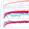Fig. 5. Measured collision kernel ⟨C⟩ normalised to (ai + aj)3. Panel a: case of constant (initial) ai, while panel b: case where (ai + aj)3 evolves and where ℳrms is also included in the normalisation. The simulations are the same as in Fig. 2. Panel c: same normalisation as panel b, but with ℳp,rms.

According to Fig. 5a, ⟨C_ij⟩ exhibits a clear increase from subsonic to supersonic turbulence (cf. ℳ_rms = 0.55, cyan curve in Fig. 5a and ℳ_rms = 2.58, red curve in Fig. 5a). As we argued in Sect. 3.3, ⟨C_ij⟩ is proportional to ℳ_rms under the assumption of Maxwellian velocity distributions. Figure 5b shows ⟨C_ij⟩ normalised also by ℳ_rms. We note that a linear scaling seems to be applicable from the subsonic regime to the supersonic regime. This means that the simple analytical theory is reasonable. The cyan curve deviates from other curves because the initial Stokes number for this simulation is about 10, as listed in Table 1. The Stokes number dependence of ⟨C_ij⟩ can be further confirmed by Fig. 5c. As ⟨C_ij⟩ is determined by the relative velocity of colliding pairs, we normalised ⟨C_ij⟩ by v_p, rms/c_s, as shown in Fig. 5c. It is obvious that ⟨C_ij⟩ scales linearly with v_p, rms/c_s up to the supersonic regime. Figure 6 shows the distribution of the magnitudes of the particle velocities, which indeed is very similar to a Maxwellian velocity distribution. It also shows that particle velocities become higher with increasing ℳ_rms. Especially the tail of the particle velocity distribution becomes more populated. This indicates that stronger shocks accelerate inertial particles more and may therefore increase the coagulation rate.

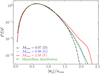Fig. 6. Particle velocity distribution at 105τL. The dashed line is a Maxwellian fit of the particle velocity of run G.

According to Eq. (19), the collision kernel is determined by the relative velocity w_ij and the relative separation Δr of two colliding particles. The former scenario is known as caustics (Wilkinson et al. 2006) and the latter as clustering (Gustavsson & Mehlig 2016), as discussed above. Our simulations involve coagulation, which leads to evolution of α(a, t). This makes it difficult to analyse clustering and caustics based on these simulations. Below we try to understand the ℳ_rms-dependence based on the spatial distribution and velocity statistics of the particles.

As shown in Fig. 7, the spatial distribution of particles exhibits different behaviours in the three α ranges we considered. When α < 0.1, particles tend to be trapped in regions where high gas density occurs. This is consistent with the findings of Hopkins & Lee (2016) and Mattsson et al. (2019b), even though coagulation was not considered in their studies. When 0.1 ≤ α ≤ 0.3, particles still accumulate in the high-density regions, but are also spread out in regions with low gas density. This dispersion is expected as τ_i increases. Finally, when α > 0.3, particles more or less decouple from the flow, demonstrating essentially a random-walk behaviour. When we compare with ℳ(x,t) instead of lnρ, we see that particles accumulate in regions with low local ℳ(x,t), as shown in Fig. 8. That is, low ℳ(x,t) corresponds to high lnρ(x, t). The physical picture is the following. Strong shocks generated in these local supersonic regions push particles to low ℳ(x,t) regions, which is then how particle densities increase due to compression of the gas. This compaction of particles is different from the fractal clustering of inertial particles, which mainly occurs as a result of accumulation of particles in the convergence zones between vortices. Statistically, the spatial distribution of particles can be characterised by g(r), which contributes to the mean collision rate as expressed in Eq. (19). However, g(r) is only useful as a diagnostic for a mono-dispersed particle distribution or fixed size bins (Pan et al. 2011). Therefore we only show the spatial distributions of particles and do not go into details about the quantitative statistics.

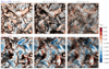Fig. 7. Spatial distribution of inertial particles and the gas density at 80 time units in a slab with thickness η for run F.

Fig. 8. Same as Fig. 7, but with ℳ(x,t) as the contour map.

As the collision kernel ⟨C_ij⟩ is also determined by |w_ij|, we also examined the magnitude of particle velocities for different ranges of α. Figure 9 shows the PDF of |v_p|/u_rms for α < 0.1, 0.1 ≤ α ≤ 0.3, and α > 0.3, respectively. It is evident that the velocity magnitude of particles that are coupled to the flow is higher than that of particles that are decoupled from the flow. Thus, the ℳ_rms dependence of ⟨C_ij⟩ could very well be due to enhanced caustics and compression-induced concentration with increasing ℳ_rms.

Fig. 9. Corresponding PDF for Fig. 7.

In incompressible turbulence, the collision kernel depends on τ_η, which is determined by $⟨\overline{ϵ}⟩$, while it is insensitive to Re (Grabowski & Wang 2013; Li et al. 2018). We examined the $⟨\overline{ϵ}⟩$ and Re dependences of a₂₄ and σ_a in compressible turbulence. As shown in Fig. 10, a₂₄ and ${\sigma }_a/\stackrel{\sim }{a}$ have only a weak dependence on $⟨\overline{ϵ}⟩$ in the supersonic regime (e.g. simulations A and C have similar ℳ_rms but differ by a factor of two in $⟨\overline{ϵ}⟩$). By inspection of Fig. 10, changing Re (run H and I) does not obviously affect a₂₄ and ${\sigma }_a/\stackrel{\sim }{a}$ in the transonic regime, which may seem to be consistent with the simulation results for incompressible turbulence.

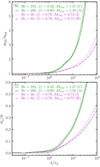Fig. 10. Time evolution of (a) a24 and (b) dispersion of f(a, t) for different $⟨\overline{ϵ}⟩$ and Re with the same ℳrms (see runs A, C, H, and I in Table 1).

5. Discussion

We have observed that as ℳ_rms increases, the tail of the distribution increases. This poses mainly two questions: (1) how the compression-induced density variation (simply compaction) affects ⟨R_ij⟩, and (2) how the velocity dispersion of particles due to shocks affects ⟨C_ij⟩.

According to Eq. (19), the coagulation rate ⟨R_ij⟩ is determined by g(a, r) and |w_ij|, as discussed in Sect. 4. Particles tend to stay in regions where the gas density is high due to shock-induced compaction. With larger ℳ_rms, the gas density fluctuations become stronger. This leads to somewhat higher concentrations of particles, especially for particles with α ≤ 0.3. It is important to note that particles accumulate in low ℳ(x,t) regions, where the gas density is high because particles are pushed to lower ℳ(x,t) regions by the shocks. Supersonic flows cover a wide range of ℳ(x,t), which results in stronger density variations of particles. Local concentrations of particles might lead to higher ⟨R_ij⟩. Therefore the enhanced ⟨R_ij⟩ with increasing ℳ_rms is indeed due to the change in the flow structure. In addition to the compressibility, fractal clustering due to inertia effect (large St) of particles might also enhance ⟨C_ij⟩.

Higher ℳ_rms results in stronger shocks and thus higher particle velocities, which also leads to larger ⟨C_ij⟩. In particular, for supersonic flows, the local fluctuations of ℳ(x,t) are strong. This leads to significant local dispersion in the particle velocities and a consequent enhancement of ⟨C_ij⟩. The coagulation rate time series almost collapse on top of each other when normalised by v_p, rms/c_s up to the supersonic regime. This indicates that the simple description of the collision kernel, Eq. (23), applies up to the supersonic regime. As particles grow larger in the simulation, they decouple from the flow. Statistically, this decoupling can be roughly described by the difference between u_rms and v_p, rms. This probably causes these curves to collapse on each other when ⟨C_ij⟩ is normalised by v_p, rms/c_s. We therefore propose that ⟨C_ij⟩ is proportional to v_p, rms/c_s instead of ℳ_rms in Eq. (23).

Since the inertial range is determined by Re, we also examined how ⟨C_ij⟩ depends on Re. As shown in Fig. 10, the Re dependence is weak because τ_i ≪ τ_L. Pan & Padoan (2014) have suggested that the collision kernel is independent of Re in the subsonic regime. We show here that this also appears to apply to the transonic regime and likely also the supersonic regime. As we discussed in Sect. 2.1, for incompressible turbulence, ⟨C_ij⟩ is determined by $⟨\overline{ϵ}⟩$ through τ_η. Figure 10 shows that the $⟨\overline{ϵ}⟩$ dependence observed in incompressible flows vanishes in compressible flows, however, which is quite expected. We demonstrated that the coagulation rate of inertial particles is mainly affected by ℳ_rms, essentially the level of compression of the flow. We conclude that ℳ_rms is the main parameter determining ⟨C_ij⟩ in the trans- and supersonic regimes.

The pioneering work of Saffman & Turner (1956) suggested that $\langle C_i\rangle \sim {\tau }_{\eta }^{-1}$ for specified sizes of particles. Because ${\tau }_{\eta }={(\nu /⟨\overline{ϵ}⟩)}^{1/2}$, $⟨C_i⟩\sim {⟨\overline{ϵ}⟩}^{1/2}$, which has been confirmed in many studies of incompressible turbulence. More importantly, all simulation works have found that ⟨C_i⟩ is independent of Re (see Grabowski & Wang 2013; Li et al. 2018 and the references therein). This is contradictory, however, because $⟨\overline{ϵ}⟩$ is a parameter that is determined by Re. We argue that this is because of the forcing term in the N-S equation, which is inevitable in turbulence simulations. This forcing term invokes a third dimensional parameter $⟨\overline{ϵ}⟩$ that determines ⟨C_i⟩ in incompressible turbulence. For compressible turbulence, however, our study showed that ⟨C_i⟩ is determined by ℳ_rms alone and independent of $⟨\overline{ϵ}⟩$. We can then avoid the contradiction described above. However, this contradiction is a more fundamental problem that requires a solution, but this is beyond the scope of our study. In short, compressible turbulence implies that $⟨\overline{ϵ}⟩$ is not only determined by Re, but also by ℳ_rms. Even though $⟨\overline{ϵ}⟩$ does not affect ⟨C_i⟩ directly, it affects the Stokes number St = τ_i/τ_η. Therefore the ⟨C_i⟩ time series collapse on top of each other when they are normalised by τ_η in Fig. 5c.

Andersson et al. (2007) proposed that in 2D compressible flow with a Gaussian random velocity, fractal particle (inertialess) clustering can lead to a higher coagulation rate. In addition to the aforementioned assumptions, the collision rate suggested in Andersson et al. (2007) involves the fractal dimension D₂, which is difficult to measure in our case because we have an evolving size distribution of particles. A direct comparison between our simulation and the theory of Andersson et al. (2007) is therefore not feasible. Nevertheless, we do observe fractal clustering in our simulation, which could indeed elevate the coagulation rate because Fig. 6 shows that high ℳ_rms flow results in higher particle velocities. Because we have a wide range of Stokes numbers, the fractal clustering (Falkovich et al. 2001) could also be enhanced.

6. Summary and conclusion

Coagulation of inertial particles in compressible turbulence was investigated by direct and shock-capturing numerical simulations. Particle interaction was tracked dynamically in a Lagrangian manner, and the consequential coagulation events were counted at each simulation time step. We specifically explored the Mach-number dependence of the coagulation rate and the effects on the widening of the particle-size distribution. To our knowledge, this is the first time that this has been done.

We showed that the coagulation rate is determined by Mach number ℳ_rms in compressible turbulence. This is fundamentally different from the incompressible case, where the coagulation rate is mainly determined by $⟨\overline{ϵ}⟩$ through the Kolmogorov timescale.

The dispersion or variance of f(a, t), σ_a, increases with increasing ℳ_rms. We also note that σ_a is a simple and more or less universal function of the size of the largest particles, measured by a₂₄, and is apparently independent of ℳ_rms.

All effects on coagulation increase progressively with ℳ_rms, which shows the importance of compressibility for coagulation processes. Taken at face value, our simulations appear to suggest that existing theories of the ℳ_rms dependence of ⟨C_ij⟩, which imply an underlying linear scaling with ℳ_rms, are correct to first order, but we cannot draw any firm conclusions at this point. For this we will need more simulations with a wider range of ℳ_rms values. We note that ⟨C_ij⟩ scales as ⟨C_ij⟩∼(a_i + a_j)³ ℳ_rms/τ_η. When the collision kernel ⟨C_ij⟩ is normalised by v_p, rms/c_s, the curves collapse on top of each other. We therefore suggest that ⟨C_ij⟩ is proportional to v_p, rms/c_s, rather than ℳ_rms. This finding may serve as a benchmark for future studies of coagulation of dust grains in highly compressible turbulence.

We propose two mechanisms that might be behind the ℳ_rms dependence of the broadening of f(a, t) even though it is still not fully understood due to the non-equilibrium nature of the coagulation process in compressible turbulence. The first mechanism is the compaction-induced concentration of particles. Supersonic flow exhibits stronger fluctuations of local ℳ(x,t). The consequent vigorous shocks compact small particles (e.g. α < 0.3) into low-ℳ(x,t) regions. This leads to high densities of particles (n_i) and then potentially to a higher coagulation rate ⟨R_ij⟩. The second mechanism is larger dispersion of particle velocities caused by stronger shocks. Again, stronger local fluctuations ℳ(x,t) lead to a larger dispersion of particle velocities, which increases the coagulation rate.

Simulating the coagulation problem in compressible and supersonic turbulence, we achieved ℳ_rms = 2.58, but with a non-astrophysical scaling. This is smaller than the ℳ_rms ≥ 10 observed in cold clouds. To explore whether a saturation limit of the ℳ_rms dependence of the coagulation rate exists, a direct numerical simulation coupled with coagulation would have to reach at least ℳ_rms ∼ 10.

We also note that the simulated systems in our study have flow timescales (turn-over times) that are of the same order as the coagulation timescale, that is, τ_c/τ_L < 1, which is computationally convenient, but very different from dust in the ISM, for example, where τ_c/τ_L ≫ 1. Nonetheless, our study provides a benchmark for simulations of dust-grain growth by coagulation in the ISM and other dilute astrophysical environments.

Reaching really high ℳ_rms, and astrophysical scales in general is currently being explored. Fragmentation is also omitted in this study, which may overestimate the coagulation rate. Adding fragmentation is a topic for future work.

Acknowledgments

Xiang-Yu Li wishes to thank Axel Brandenburg, Nils Haugen, and Anders Johansen for illuminating discussions about the simulation code used in this study, the PENCIL CODE. Lars Mattsson wishes to thank the Swedish Research Council (Vetenskapsrdet, grant no. 2015-04505) for financial support. We thank the referee for very helpful suggestions to improve the manuscript. Our simulations were performed using resources provided by the Swedish National Infrastructure for Computing (SNIC) at the Royal Institute of Technology in Stockholm, Linköping University in Linköping, and Chalmers Centre for Computational Science and Engineering (C3SE) in Gothenburg. The PENCIL CODE is freely available on https://github.com/pencil-code/. The authors also thank the anonymous reviewer for constructive comments on the paper.

References

Appendix A: Coagulation kernel: An alternative expression

This appendix presents a discussion of an alternative description of the coagulation rate and the underlying mechanisms. Equation (19) appears to be a natural expression for the collision kernel between particle pairs. However, it is not a physically complete and always representative model (Wilkinson et al. 2006). Two mechanisms contribute to the collision kernel C_ij due to particle inertia: clustering and caustics. The former is characterised by g(r) ∝ r^{D₂ − d} at a fixed Stokes number, where g is the radial distribution function, d is the spatial dimension, and D₂ is the correlation dimension (Reade & Collins 2000; Grassberger & Procacia 1983). The latter is the effect of singularities in the particle phase space at non-zero values of the Stokes number (Falkovich et al. 2002; Wilkinson et al. 2006; Gustavsson & Mehlig 2014). It appears when phase-space manifolds fold over. In the fold region, the velocity field at a given point in space becomes multi-valued, allowing for large velocity differences between nearby particles, which results in a temporarily increased particle-interaction rate and more efficient coagulation (Gustavsson & Mehlig 2014). As indicated above, the relative velocity between two colliding pairs obeys a power law |⟨w_ij⟩| ∝ (r_i + r_j)^{d − D₂}. Thus, the product of g(r) and |⟨w_ij⟩| is independent of (r_i + r_j), that is, caustics and clustering cancel each other out in this formulation. Therefore Wilkinson et al. (2006) proposed that C_ij is a superposition of clustering and caustics, which was confirmed by numerical simulations (Voßkuhle et al. 2014). In Sect. 3.3 of our study we ignored the effects of caustics mainly because caustics in high ℳ_rms compressible turbulence are associated with shock interaction and density variance in the carrier fluid, in which case the resultant increase in particle number density is a far greater effect than the caustics.

All Tables

All Figures

	Fig. 1. Power spectra for simulations of different ℳrms: ℳrms = 0.07 (solid dotted black curve), 0.55 (dashed cyan curve), 0.99 (dotted blue curve), and 2.58 (red curve). The dashed black curve shows the Kolmogorov −5/3 law.
In the text

	Fig. 2. Time evolution of f(a, t) for simulations in Fig. 1 and for an additional simulation run H in Table 1.
In the text

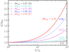	Fig. 3. Time evolution of $\stackrel{\sim }{a}/a_{\mathrm{ini}}$ for simulations in Fig. 2.
In the text

	Fig. 4. Time evolution of (a) the a24 and (b) ${\sigma }_a/\stackrel{\sim }{a}$ for simulations in Fig. 2. The inset shares the same y-axis as the main plot in panel b. The dashed magenta curve in the inset shows ln(a24/aini).
In the text

	Fig. 5. Measured collision kernel ⟨C⟩ normalised to (ai + aj)3. Panel a: case of constant (initial) ai, while panel b: case where (ai + aj)3 evolves and where ℳrms is also included in the normalisation. The simulations are the same as in Fig. 2. Panel c: same normalisation as panel b, but with ℳp,rms.
In the text

	Fig. 6. Particle velocity distribution at 105τL. The dashed line is a Maxwellian fit of the particle velocity of run G.
In the text

	Fig. 7. Spatial distribution of inertial particles and the gas density at 80 time units in a slab with thickness η for run F.
In the text

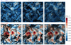	Fig. 8. Same as Fig. 7, but with ℳ(x,t) as the contour map.
In the text

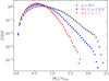	Fig. 9. Corresponding PDF for Fig. 7.
In the text

	Fig. 10. Time evolution of (a) a24 and (b) dispersion of f(a, t) for different $⟨\overline{ϵ}⟩$ and Re with the same ℳrms (see runs A, C, H, and I in Table 1).
In the text

References

- Abrahamson, J. 1975, Chem. Eng. Sci., 30, 1371 [Google Scholar]
- Aldous, D. J. 1999, Bernoulli, 5, 3 [Google Scholar]
- Andersson, B., Gustavsson, K., Mehlig, B., & Wilkinson, M. 2007, EPL (Europhys. Lett.), 80, 69001 [Google Scholar]
- Armitage, P. J. 2010, Astrophysics of Planet formation (Cambridge University Press) [Google Scholar]
- Bec, J. 2003, Phys. Fluids, 15, L81 [Google Scholar]
- Bec, J. 2005, J. Fluid Mech., 528, 255 [Google Scholar]
- Bec, J., Cencini, M., & Hillerbrand, R. 2007a, Phys. Rev. E, 75, 025301 [Google Scholar]
- Bec, J., Biferale, L., Cencini, M., et al. 2007b, Phys. Rev. Lett., 98, 084502 [Google Scholar]
- Bhatnagar, A., Gustavsson, K., & Mitra, D. 2018, Phys. Rev. E, 97, 023105 [Google Scholar]
- Bird, G. 1978, Annu. Rev. Fluid Mech., 10, 11 [Google Scholar]
- Bird, G. 1981, Prog. Astronaut. Aeronaut., 74, 239 [Google Scholar]
- Birnstiel, T., Fang, M., & Johansen, A. 2016, Space Sci. Rev., 205, 41 [Google Scholar]
- Bourdin, P.-A. 2020, Geophys. Astrophys. Fluid Dynam., 114, 235 [Google Scholar]
- Brandenburg, A. 2001, ApJ, 550, 824 [Google Scholar]
- Brandenburg, A., & Dobler, W. 2002, Comput. Phys. Commun., 147, 471 [Google Scholar]
- Brandenburg, A., Johansen, A., Bourdin, P., et al. 2021, J. Open Source Softw., 6, 2807 [Google Scholar]
- Draine, B. T., & Salpeter, E. E. 1979, ApJ, 231, 438 [Google Scholar]
- Eaton, J., & Fessler, J. 1994, Int. J. Multiphase Flow, 20, 169 [Google Scholar]
- Elmegreen, B. G., & Scalo, J. 2004, ARA&A, 42, 211 [NASA ADS] [CrossRef] [Google Scholar]
- Falkovich, G., Gawedzki, K., & Vergassola, M. 2001, Rev. Mod. Phys., 73, 913 [Google Scholar]
- Falkovich, G., Fouxon, A., & Stepanov, M. 2002, Nature, 419, 151 [Google Scholar]
- Federrath, C., Klessen, R. S., & Schmidt, W. 2009, ApJ, 692, 364 [Google Scholar]
- Federrath, C., Roman-Duval, J., Klessen, R. S., Schmidt, W., & Mac Low, M.-M. 2010, A&A, 512, A81 [NASA ADS] [CrossRef] [EDP Sciences] [Google Scholar]
- Grabowski, W. W., & Wang, L.-P. 2013, Annu. Rev. Fluid Mech., 45, 293 [Google Scholar]
- Grassberger, P., & Procacia, I. 1983, Physica. D, 9, 189 [Google Scholar]
- Gustavsson, K., & Mehlig, B. 2014, J. Turbul., 15, 34 [Google Scholar]
- Gustavsson, K., & Mehlig, B. 2016, Adv. Phys., 65, 1 [Google Scholar]
- Haugen, N. E. L., Brandenburg, A., & Mee, A. J. 2004, MNRAS, 353, 947 [Google Scholar]
- Hirashita, H. 2010, MNRAS, 407, L49 [NASA ADS] [Google Scholar]
- Hirashita, H., & Yan, H. 2009, MNRAS, 394, 1061 [Google Scholar]
- Hirashita, H., Asano, R. S., Nozawa, T., Li, Z.-Y., & Liu, M.-C. 2014, Planet. Space Sci., 100, 40 [Google Scholar]
- Hopkins, P. F., & Lee, H. 2016, MNRAS, 456, 4174 [Google Scholar]
- Johansen, A., & Lambrechts, M. 2017, Annu. Rev. Earth Planet. Sci., 45, 359 [Google Scholar]
- Johansen, A., Youdin, A. N., & Lithwick, Y. 2012, A&A, 537, A125 [NASA ADS] [CrossRef] [EDP Sciences] [Google Scholar]
- Jorgensen, W. L., Chandrasekhar, J., Madura, J. D., Impey, R. W., & Klein, M. L. 1983, J. Chem. Phys., 79, 926 [Google Scholar]
- Klett, J., & Davis, M. 1973, J. Atmos. Sci., 30, 107 [Google Scholar]
- Kwok, S. 1975, ApJ, 198, 583 [Google Scholar]
- Li, X.-Y., Brandenburg, A., Haugen, N. E. L., & Svensson, G. 2017, J. Adv. Model. Earth Syst., 9, 1116 [Google Scholar]
- Li, X.-Y., Brandenburg, A., Svensson, G., et al. 2018, J. Atmos. Sci., 75, 3469 [Google Scholar]
- Li, X.-Y., Brandenburg, A., Svensson, G., et al. 2020, J. Atmos. Sci., 77, 337 [Google Scholar]
- Mattsson, L. 2011, MNRAS, 414, 781 [Google Scholar]
- Mattsson, L. 2016, P&SS, 133, 107 [Google Scholar]
- Mattsson, L., Bhatnagar, A., Gent, F. A., & Villarroel, B. 2019a, MNRAS, 483, 5623 [Google Scholar]
- Mattsson, L., Fynbo, J. P. U., & Villarroel, B. 2019b, MNRAS, 490, 5788 [Google Scholar]
- Maxey, M. R. 1987, J. Fluid Mech., 174, 441 [Google Scholar]
- Pan, L., & Padoan, P. 2013, ApJ, 776, 12 [Google Scholar]
- Pan, L., & Padoan, P. 2014, ApJ, 797, 101 [Google Scholar]
- Pan, L., & Padoan, P. 2015, ApJ, 812, 10 [Google Scholar]
- Pan, L., Padoan, P., Scalo, J., Kritsuk, A. G., & Norman, M. L. 2011, ApJ, 740, 6 [Google Scholar]
- Pan, L., Padoan, P., & Scalo, J. 2014a, ApJ, 791, 48 [Google Scholar]
- Pan, L., Padoan, P., & Scalo, J. 2014b, ApJ, 792, 69 [Google Scholar]
- Passot, T., & Vázquez-Semadeni, E. 1998, Phys. Rev. E, 58, 4501 [Google Scholar]
- Price, D. J., Federrath, C., & Brunt, C. M. 2011, ApJ, 727, L21 [Google Scholar]
- Reade, W. C., & Collins, L. R. 2000, Phys. Fluids, 12, 2530 [Google Scholar]
- Rowlands, K., Gomez, H. L., Dunne, L., et al. 2014, MNRAS, 441, 1040 [Google Scholar]
- Saffman, P. G., & Turner, J. S. 1956, J. Fluid Mech., 1, 16 [Google Scholar]
- Schaaf, S. A. 1963, Handbuch der Physik, 3, 591 [NASA ADS] [Google Scholar]
- Smoluchowski, M. V. 1916, Zeitschrift fur Physik, 17, 557 [Google Scholar]
- Squires, K. D., & Eaton, J. K. 1991, Phys. Fluids A Fluid Dyn., 3, 1169 [Google Scholar]
- Sundaram, S., & Collins, L. R. 1997, J. Fluid Mech., 335, 75 [Google Scholar]
- Valiante, R., Schneider, R., Salvadori, S., & Bianchi, S. 2011, MNRAS, 416, 1916 [Google Scholar]
- Voßkuhle, M., Pumir, A., Lévêque, E., & Wilkinson, M. 2014, J. Fluid Mech., 749, 841 [Google Scholar]
- Wang, L.-P., Wexler, A. S., & Zhou, Y. 2000, J. Fluid Mech., 415, 117 [Google Scholar]
- Wilkinson, M., & Mehlig, B. 2005, EPL (Europhys. Lett.), 71, 186 [Google Scholar]
- Wilkinson, M., Mehlig, B., & Bezuglyy, V. 2006, Phys. Rev. Lett., 97, 048501 [Google Scholar]
- Yavuz, M. A., Kunnen, R. P. J., van Heijst, G. J. F., & Clercx, H. J. H. 2018, Phys. Rev. Lett., 120 [Google Scholar]
- Zsom, A., & Dullemond, C. P. 2008, A&A, 489, 931 [NASA ADS] [CrossRef] [EDP Sciences] [Google Scholar]