| Issue |
A&A
Volume 648, April 2021
|
|
|---|---|---|
| Article Number | A67 | |
| Number of page(s) | 14 | |
| Section | Atomic, molecular, and nuclear data | |
| DOI | https://doi.org/10.1051/0004-6361/202038254 | |
| Published online | 13 April 2021 | |
Electron-impact excitation of Ni II
Centre for Theoretical Atomic, Molecular and Optical Physics, Queen’s University Belfast, University Road,
Belfast,
BT7 1NN,
UK
e-mail: This email address is being protected from spambots. You need JavaScript enabled to view it.
Received:
24
April
2020
Accepted:
26
February
2021
Abstract
Aims. Energy levels, transition probabilities, and oscillator strengths are calculated for the second most abundant iron peak element Ni II. The difficulty in obtaining an accurate target representation is related to the open d-shell nature of the target, which has a minimum requirement of single and double promotions from the ground state configuration to the n = 4 shells. Therefore, in order to achieve an accurate representation of the target ion, we have also included configurations containing the 4d, 5s, and 5p subshells. We have undertaken a study of the electron impact excitation of Ni II and present here the collision strengths for forbidden and allowed transitions among the lowest 800 fine-structure levels as well as the corresponding Maxwellian-averaged effective collision strengths for a range of astrophysically relevant electron temperatures.
Methods. An accurate Ni II target structure was generated using the modified General-purpose Relativistic Atomic Structure Package (GRASP0) for the lowest lying 1220 jj fine-structure levels, comprising the 11 configurations: 3p63d9, 3p63d84s, 3p63d84p, 3p63d84d, 3p63d85s, 3p63d85p, 3p63d74s2, 3p63d75s2, 3p63d74s4p, 3p63d74s4d, and 3p43d94s4d. The relativistic parallel Dirac atomic R-matrix codes (DARC) were utilised in the scattering calculations to generate the collision strengths for incident electron energies between 0 and 2 Ryd and, by employing infinite dipole and non-dipole limit points, we also generated the effective collision strengths for temperatures in the range from 1000 to 400 000 K. Two separate calculations were performed, both comprised of truncated close-coupling expansions of 800 jj-levels with the first calculation retaining the theoretical ab initio energy levels generated in the GRASP0 evaluations, whereas in the second calculation these energies were shifted to their predicted National Institute of Standards and Technology (NIST) values where possible. This should provide a lower estimate on the uncertainty.
Results. Comparisons are made between the radiative data and the collisional cross sections with past theoretical and experimental studies. The effective collision strengths when compared with the most recent published calculations, are found to agree to within 10% for the majority of the transitions considered. In addition, the data are used to model the spectrum of Ni II and good agreement is found with previous investigations and observations.
Key words: atomic data / atomic processes / relativistic processes / line: identification
© ESO 2021
1 Introduction
Atomic structure and collisional calculations provide the theoretical groundwork that underpins the interpretation of astrophysical spectra, allowing astrophysicists to accredit particular atomic ions to a wide range of astrophysical objects. Atomic data of particular interest are those elements which are highly abundant and routinely observed in nebular spectroscopy, including ions such as the Fe-peak elements Fe, Co, and Ni. Of these Fe-peak elements, Ni II is the second most abundant. Unfortunately, there is a lack of accurate atomic data available in the literature pertaining to this ion and hence the demand for precise and accurate data for singly ionised Ni is evident and paramount.
Emission lines for Ni II have been observed in a variety of different astrophysical sources. These include filaments of the luminous blue variable (LBV) star, known as η Carinae (Davidson et al. 2001), where emission lines were observed even for forbidden transitions. Other sources are stars which have evolved to be red giants (Richardson et al. 2011), and if such stars do not have a large enough mass to evolve into a neutron star, they become white dwarfs (Klein et al. 2011), which are another example of such a source. The spectra of galaxies, known as Seyfert galaxies, have also shown lines of Ni II (Véron-Cetty et al. 2006). A further example are γ-ray bursts, where Ni II lines have been observed using high resolution spectroscopy Cucchiara et al. (2011). As Ni II is an abundant Fe-peak element and can be observed in such a variety of astrophysical objects, it is not surprising that there have been numerous experimental studies over the last several decades. In more recent years, lines of the Ni II spectrum have been observed in ultraviolet (UV) and vacuum ultraviolet (VUV) spectral ranges. Specifically, Ferrero et al. (1997) observed UV lines in the wavelength region from 2100–2600 Å and subsequently measured the transition probabilities for these lines. Following this work, Zsargó & Federman (1998) observed VUV lines in the wavelength range from 1300–1750 Å. They presented f-values for 12 resonance lines within this range and when compared with the work of Morton (1991) (which later became the standard data in the National Institute of Standards and Technology: NIST, Kramida et al. 2019), agreement was found for the strong transitions but discrepancies remained for the weaker lines.
Additional studies of UV and VUV lines of Ni II were undertaken by Fedchak & Lawler (1999). They observed 59 lines in the range from 1700–2550 Å and presented absolute transition probabilities for each line. They contrasted their work to that of Zsargó & Federman (1998) by using a scaling factor (0.534 ± 10%) to present their results on an absolute scale. Fedchak et al. (2000) extended this work by presenting relative f-values for resonance lines to a higher degree of accuracy. Further work was carried out by Dessauges-Zavadsky et al. (2006), where they included an additional transition (3d9 2 D5∕2–3d8(1G)4p 2F ) at λ = 1317 Å omitted from the work of Fedchak et al. (2000). This transition was due to a single electron promotion from the 3d to the 4p orbital and the value of the oscillator strength was subsequently confirmed by the experiments of Jenkins & Tripp (2006) at a wavelength of λ = 1317 Å.
Open d-shell systems give rise to hundreds of target levels. This presents difficulties not only in achieving an accurate structure model, but also computationally due to the large number of close-coupling channels required in the subsequent collisional calculations. The earliest theoretical calculations for Ni II were those of Gruzdev (1962) and Mendlowitz (1966), both of which calculated intermediate coupling transition probabilities for several emission lines of Ni II. Not until Nussbaumer & Storey (1982) carried out their investigation of Ni II were the first electron excitation rates calculated. These calculations were restricted, however, as they did not include resonances in the collision cross sections and may have underestimated the contributions from broad resonance features to Maxwellian-averaged collision strengths. Calculations that followed were based on the package COWAN (Cowan 1981). For example the work of Kurucz (2000) produced the most thorough theoretical study of Ni II at that time using this semi-relativistic technique.
An early R-matrix calculation was presented in the work of Bautista & Pradhan (1996) who investigated the electron impact excitation of Ni II using a structure containing two basis configurations (3p6 3d9 and 3p6 3d84s) which resulted in a seven LS term, 17 jj-level fine structure evaluation. Results from this work showed some agreement with earlier predictions of Nussbaumer & Storey (1982) for the strong lines but were found to be significantly different for weak transitions. Watts et al. (1996) carried out a further study incorporating a larger three configuration basis (+3p63d84p) but this calculation was carried out only in LS coupling. Bautista (2004) included four basis configurations, the ground configuration, a single promotion of the 3d orbital to the 4s and 4p configurations and a double promotion of the 3d orbitals to the 4s2 configuration (3p6 3d9, 3p6 3d84s, 3p6 3d84p, 3p6 3d74s2). These earlier models focused on low temperature diagnostics as compared to the work presented here which has a wider scope of application. The most recent and largest theoretical R-matrix calculation for Ni II was completed by Cassidy et al. (2010) using an extended version of the R-matrix code (RMATRX II). Their work comprised of a model incorporating 295 fine-structure levels constructed from five configurations, 3p6 3d9, 3p6 3d84s, 3p6 3d84p, 3p6 3d74s2, and 3p6 3d74s4p. In this work energy levels, oscillator strengths, collision strengths and effective collision strengths were presented for a wide range of incident electron energies and electron temperatures. In addition, Cassidy et al. (2016) completed an extensive study on the radiative atomic data for Ni II leading to the identification of weak transitions at 1502, 1773, and 1804 Å by Boissé & Bergeron (2019), who carried out an experimental study of the oscillator strengths for 13 Ni II transitions. Furthermore, Cassidy et al. (2011) calculated effective collision strengths from the work already detailed in their previous paper (Cassidy et al. 2010).
This paper will comprise of a new calculation for the Fe-peak element Ni II. The impetus for this more extensive data set, which includes significantly more levels, was highlighted by Leighly et al. (2007), which reported on observations of the unusually bright, luminous, nearby narrow-line quasar PHL 1811. It was found that the near UV-spectrum was dominated by very strong low ionisation stages of Fe-peak ions such as Ni II. However, the data sets available to Leighly et al. (2007) were limited, and in particular the CLOUDY (Ferland et al. 2017) models were inadequate to model the line emission spectrum in detail, particularly at higher energies.
In this paper we present two calculations, the first a five configuration model to provide a benchmark for comparison with the second calculation, an extensive 11 configuration model which contains the 4d, 5s, and 5p orbitals. These high lying states have not been studied theoretically to date and will provide the necessary improvements required to accurately model astrophysical objects, such as the quasars mentioned previously.
We present in Sect. 2 energy levels, transition rates and oscillator strengths from both these structure calculations and compare with the most recent theoretical data (Kramida et al. 2019; Cassidy et al. 2016) to gauge their accuracy. Experimental oscillator strengths (Ferrero et al. 1997; Zsargó & Federman 1998; Fedchak & Lawler 1999; Fedchak et al. 2000; Jenkins & Tripp 2006) are also compared with to test accuracy. Section 3 describes an outline of the R-matrix theory that underpins these electron-impact excitation collisions. In Sect. 4 we present the electron-impact excitation collision strengths and corresponding effective collision strengths for a wide range of electron temperatures. Comparisons are made with earlier predictions and conclusions drawn. In addition, we are interested in investigating how shifting the target energies during the collision calculation can affect the resulting cross sections. Completing the calculations with and without target energy adjustments will enable us to clearly see the effect that fine-tuning the energy levels has on the final atomic data produced by the collision calculations and provides an estimate of uncertainty. In Sect. 5, we complete a preliminary study on the theoretical modelling of Ni II, by presenting a photon emissivity coefficient (PEC) plot for the spectrum of Ni II calculated using our data. A PEC of a particular transition can be described as the product of the Einstein A coefficient (A-value) and the population of the upper level within the quasi-static approximation for that transition. Comparing with previous observed works allows us to identify known spectral lines of Ni II.
2 Atomic structure
Ni II is one of the many elements that can be found in the spectra of stars and its rich energy level spectrum can be seen in Fig. 1. To achieve this we solve the relativistic Dirac equation,
 (1)
(1)
where ϕ is the Dirac orbital, and HD the Dirac Hamiltonian. The stationary states of the Dirac-Coulomb Hamiltonian (HDC) for a single electron can be defined as,
 (2)
(2)
where c is the speed of light, α and β are Dirac matrices, p is the momentum operator, and IN is the N × N identity matrix. Replacing the momentum operator, Eq. (2) can be written as,
 (3)
(3)
The Dirac matrices α and β, are defined by,
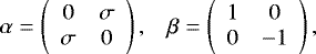 (4)
(4)
where σ is the 2 × 2 Pauli spin matrix.
In the present structure calculations we utilise the GRASP0 (General Purpose Relativistic Atomic Structure Package, Dyall et al. 1996) to create models of Ni II which were subsequently incorporated into scattering calculations using the relativistic parallel DARC codes (Dirac Atomic R-matrix Codes, Ballance 2019). GRASP0 allows us to calculate the energy levels of the target states of Ni II as well as oscillator strengths and A-values for transitions between these states. By comparing with available NIST data, and values calculated by Cassidy et al. (2016), we can gauge the accuracy of the models produced, in a similar manner described in the works of Fe II (Smyth et al. 2019), Mo I (Smyth et al. 2017), Ni III and Ni IV (Fernandez Menchero et al. 2019).
Due to the large amount of configuration interaction between many nearly degenerate states, this proves difficult in converging energy levels and oscillator strengths for radiative transitions. Hence these target states require large configuration interaction expansions for their accurate representation. The subsequent parallel DARC codes now make it feasible to incorporate these complex atomic structure models within the scattering calculation. Two models where investigated in the current study.
We created a small preliminary model to contrast with existing theoretical calculations currently within the literature and to set a benchmark by which to gauge the improvement of the second larger model. This model is similar to that of Cassidy et al. (2016), however in order to more fully develop the structure we allowed an additional single promotion from the 3d orbital to the 4d orbital. The model obtained comprised of 5 configurations,
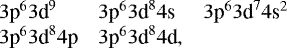
resulting in 149 jj-levels. The energy levels produced agree to within 10% of the values available in NIST for all but the lowest lying states. In terms of structure, we refer to this model as Model 1.
In the second model we expand upon Model 1 by allowing all single electron promotions to the 4s, 4p, 4d, 5s, and 5p orbitals from the 3d orbital, double promotions to the 4s and 5s orbitals from the 3d orbital, and double promotions split between the 4s and 4p (or 4d) orbitals from the 3d orbital. Lastly we include a double promotion to the 4s and 4d orbitals from the 3p orbital. This more substantial model thus comprised of the 11 configurations with the outermost 11 electrons occupying configurations as below:
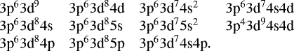
Due to the complex nature of the open d subshell this model resulted in 1220 jj fine structure levels, significantly larger than Model 1. The resulting target state energies and oscillator strengths showed an improved accuracy when compared with the NIST values. This was due to better convergence being achieved by allowing all the orbitals to be collectively variationally determined rather than converging individual orbitals one at a time. In terms of structure, we refer to this model as Model 2.
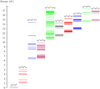 |
Fig. 1 Energy level spectrum of Ni II up to the 5p orbital, including the 4f orbital, organised by electronic configuration. Each horizontal line designates a specific fine structure level (taken from the NIST database). |
2.1 Accuracy of models
In order to evaluate the accuracy and uncertainty of our models it is important to compare our data with known reliable sources. An established method of testing accuracy of atomic structural models is to compare the energy levels and oscillator strengths with existing literature values, such as the values found in NIST.
2.1.1 Energy levels
Table 1 displays the energy levels in Ryds for the 53 lowest lying states of Ni II included in both Models 1 and 2. Comparisons are made with the energy levels from NIST only, as the data listed in the most recent publication of Cassidy et al. (2016) had already been shifted to these NIST values in preparation for the collision calculations.
Differences averaging 10.3% are found between the Model 1 energies and the NIST values for the initial 17 target states, indicating that Model 1 provides a reasonable representation for the configuration states containing a single promotion from the 3d orbital to the 4s (3p6 3d84s). The overall average absolute energy error increases to 17% once all 57 states are included. The energy levels for the odd configuration states of 3p6 3d84p are within an acceptable 10% of the NIST energies on average, however, the positions for configuration states due to the double promotion from the 3d orbital to the 4s orbital (3p6 3d74s2) exhibit much larger errors. As Model 1 contains a limited five configurations in the target wavefunction expansion, and the 3d orbital had been fixed early in the generation of the structure, this model lacks the flexibility to describe thediffering configuration states. Similarly large differences were found for the energy position of the 3p6 3d74s2 levels in the Fe-peak evaluations of Fe II (Smyth et al. 2019), Ni III and Ni IV (Fernandez Menchero et al. 2019).
In Model 2 we did not restrict any of the orbitals until all 11 of the configurations had been included. As you can see from Table 1 this substantially improves the energy levels for the 3p6 3d74s2 configuration states. The percentage error when compared to NIST reduces to a much more acceptable 8.24% on average. Improvements in nearly all the other energy levels are also evident and the overall average percentage error is found to be approximately 4.37%. We also incorporated the 5s and 5p orbitals into Model 2, this is of great interest due to the lack of available data for these higher energy levels. Table 2 presents the 20 lowest lying fine structure states containing either the 5s or 5p orbitals, comparison is made with the NIST values. Our values show excellent agreement with the existing literature having a percentage error of less than 5% from the NIST values.
2.1.2 A-values
For accuracy it is important to also compare the absorption oscillator strengths and emission transition probabilities for allowed and forbidden transitions among the target levels. Due to the incompleteness of the NIST database, a more thorough comparison is made with Cassidy et al. (2016) and where possible that of Morton (1991). In order to gauge the accuracy of our data an extensive study of comparison is completed against experimental results in existing literature (Ferrero et al. 1997; Fedchak & Lawler 1999; Fedchak et al. 2000; Zsargó & Federman 1998; Jenkins & Tripp 2006). In Table 3 and 4 we present A-values and f-values evaluated using the extensive Model 2, for a selection of important forbidden and allowed lines (which have been shifted using the atomic structure code GRASP, according to the data available in NIST), and compared with the values of Cassidy et al. (2016) and where possible the values of Morton (1991). The A-values for the transitions between the low-lying metastable levels (presented in Table 3) for Model 2 display good agreement with the values listed in Cassidy et al. (2016) with an average absolute error of 1.38E-02. From Table 4 it is evident that although the oscillator strengths do not agree to within 10% of the values listed in Cassidy et al. (2016) for a number of transitions, agreement to within the same order of magnitude is found between the two theoretical works. This is not unexpected as different approximations were employed to generate Model 2 (GRASP0) and the model presented by Cassidy et al. (2016). The former represents a fully relativistic approach whereas the latter CIV3 (Configuration Interaction code; Hibbert 1975) approach diagonalises the non-relativistic Hamiltonian and treats the relativistic effects perturbatively. In addition, the 5 configuration structure of Cassidy et al. (2016) was considerably smaller than the 11 configurations included in Model 2. However, if we focus on the transitions between the lower 3d8 4s 4 P and the 4p upper levels, agreement of around 20% is found. Better agreement is found between Model 2 and the work of Morton (1991), than between the values of Cassidy et al. (2016) and Morton (1991). Particularly if we consider the strong dipole transition between the ground state and the 3p6 3d84p 2 P
 we have an A-value of 8.46E+08 s−1 which is an order of magnitude greater than the work of Cassidy et al. (2016), but agrees much more closely with the value of Morton (1991) at 7.66E+08 s−1.
In order to further check the accuracy of the present data, an extensive comparison is presented in Table 5 of the oscillator strengths (in the length gauge) with existing experimental data. Agreement is found between our data and the experimental values for many of the transitions, in particular the 1477.22 Å is in good agreement with the observations of Zsargó & Federman (1998), and the 2158.74 and 2416.14 Å transitions also show agreement with observations of Ferrero et al. (1997) and the work of Fedchak & Lawler (1999). All other transitions display reasonable agreement.
Unfortunately, there was a lack of data available with which to draw comparisons for transitions among the 5s and 5p orbital states. In order to assess the quality of the f-values for these transitions Table 6 presents the oscillator strengths (in the length gauge) and the corresponding ratio between the velocity and length gauge of these f-values. As the ratio for these transitions is approximately 1.0, it supports the validity of these transitions.
3 Electron impact excitation
The R-matrix theory is fully described by Burke (2011) and Descouvemont & Baye (2010) and will only be summarised here. For a fully relativistic model of theN + 1 electron system we define the Dirac-Coulomb Hamiltonian as,
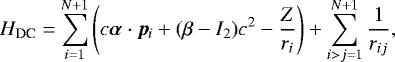 (5)
(5)
where rij = |rj − ri|. The R-matrix method partitions configuration space into two separate regions, an internal region and an external region, separated at the R-matrix boundary r = a. This boundary is chosen so that it encompasses the charge distribution of the target. We define the R-matrix as the following,
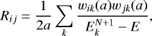 (6)
(6)
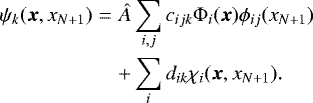
where  are the eigenenergies of the N + 1 Hamiltonian, E is the energy of the incoming electron, and wik are the surface amplitudes. Energy-independent basis functions to describe such a system are defined as the following,
 (7)
(7)
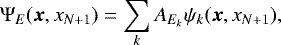
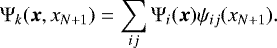
We define x = (x1, x2,..., xN) where xi = (ri, βi), ri and βi represent the position and spin state of the ith electron respectively. Â is an antisymmetrisation operator, Φi(x) are the bound states of the N-electron system, ϕij(xN+1) are the continuum orbitals, and χ(x, xN+1) are square-integrable correlation functions. We include the continuum orbitals and square-integrable functions to describe the short-range interactions between the continuum and target electrons. In the internal region, the expansion coefficients cijk and dik are obtained by diagonalising the N+1 electron Hamiltonian. These energy independent basis functions allow an eigenstate for the energy-dependent N+1 electron Hamiltonian to be obtained as follows,
 (8)
(8)
where  are energy dependent coefficients. The radial coordinates xi, where 1 ≤ i ≤ N, are within the internal region and the coordinates xN+1 are in the external region. These states are defined as,
 (9)
(9)
The collision strength between two states (initial state i and final state j) can be obtained from the cross section σi→j,
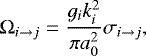 (10)
(10)
where gi is the statistical weight of the initial state wavefunction, a0 is the Bohr radius, and  is the energy of the incoming electron in Rydbergs. Obtaining a Maxwellian-convolution of the cross sections for all the transitions would allow us to see if the rate converges to the infinite energy point of the calculation. Effective collision strengths (γ) can be calculated as follows,
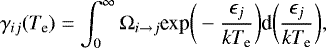 (11)
(11)
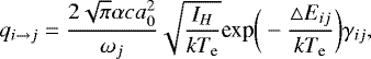
where ϵj is the energy of the scattered electron, k is the Boltzmann’s constant and Te represents the temperature of the electron in Kelvin. Using the effective collision strengths we can calculate an excitation rate coefficient (qi→j) for particular transitions,
 (12)
(12)
the corresponding de-excitation rate coefficients given by,
 (13)
(13)
where α is the fine structure constant. △ Eij is the threshold energy for the transition from level i to level j, wi and wj are statistical weights of the initial and final levels respectively, and c is the speed of light.
Energy levels (Ryd) for the lowest lying 53 fine-structure states in Ni II obtained from Models 1 and 2.
Energy levels (Ryd) for the lowest lying 31 fine-structure states containing the 5s or 5p orbital for Ni II obtained from Model 2.
A coefficients (A-values in s −1) between the metastable levels from Model 2 compared with the data from Cassidy et al. (2016).
4 Scattering calculation
4.1 Collision strengths
The 11 configurations listed in Model 2 result in a substantial 1220 fine-structure level calculation. Computationally this is challenging once incorporated into the collision evaluations. To manage the computational effort and to test convergence of the collision strengths with increasing complexity, we completed three calculations using Model 2 with successively more fine-structure levels included in the close-coupling expansion, 200 levels, 500 levels, and 800 levels. For each model, the scattering calculation was completed for an incident electron energy range from 0–2 Ryd, highlighting the importance of near threshold resonances.
In Fig. 2 we present the collision strengths as a function of incident electron energy in Rydbergs for two lines, 3d9 2D5∕2–3d9 2 D3∕2 (1–2) and 3d9 2 D5∕2–3d84s 4 F9∕2 (1–3), and in Fig. 3 we present the corresponding data for two intercombination lines, the 3d9 2 D5∕2–3d8(3F)4p 4 D (1–22) and 3d9 2D5∕2–3d8(3F)4p 4 D
 (1–23).
For the transitions presented in Fig. 2, an increased number of levels from 200 to 500 to 800 does not significantly alter the overall background cross section for either transition. Some additional strong resonance lines appear for transition 1–2 (3d9 2D5∕2–3d9 2 D3∕2) at low incident electron energies but the magnitude, behaviour and strength of the collision strength appears converged. The same cannot be said for the intercombination lines presented in Fig. 3. For both transitions, the inclusion of additional levels from 200 to 500 results in a reduction of the background cross section, particularly as we move to higher energies. A much smaller decrease is evidenced by the inclusion of levels 500 to 800, indicating convergence to the wavefunction representation for target descriptions of this size. By including 800 levels in the expansion of the target wavefunction we ensure convergence in the collision cross sections up to 2.0 Ryd relative to the ground state.
As well as the target description, convergence in the partial wave expansion may be tested by investigating the required number of Jπ partial waves required to achieve convergence, particularly for the slow converging dipole allowed lines. We present in Fig. 4 two such dipole transitions, 3d9 2 D5∕2–3d8(3F)4p 2 P (1–51) and 3d9 2 D5∕2–3d8(3F)4p 2 D
 (1–39). Three calculations, including successively larger numbers of Jπ partial waves from 20 to 40 to 60 were analysed. For both, including all partial waves up to J = 60 with even and odd parity, secures a satisfactory level of convergence and accuracy.
The cross sections were computed for a very fine energy mesh (10−3 Ryds) in the resonance region to ensure that all resonance features have been properly resolved, from 0 to 2 Ryd. The scattering computations were performed twice, one retaining the ab initio energy levels from GRASP0 and then repeated with the energies shifted to their predicted NIST values before we diagonalised the Hamiltonian. The result of shifting versus not shifting energy values will be explored through comparison of effective collision strengths, as we can draw comparison with the work of Cassidy et al. (2011) and Bautista (2004).
4.2 Effective collision strengths
The collision strengths between two states, defined by Eq. (10) and depicted in Figs. 2–4 graphically show that strong autoionising resonances, which often occur at energies below the ionisation threshold, can cause the Ωij to vary widely from the non-resonant background. For this reason many astrophysicists and plasma modellers prefer to use thermally or Maxwellian-averaged effective collision strengths, γij, defined in Eq. (11), for a range of electron temperatures of importance. We present in Figs. 5 and 6 these effective collision strengths for several transitions and for temperatures in the range from log Te = 3.0 to 6.0 K. In order to predict the effective collision strength values for the higher temperatures we extrapolated the results from the lower temperature range. As the scattering computations were performed twice for each model, we will present the effective collision strengths for all sets of data. The shifted data sets were calculated by adjusting the energy values to their predicted NIST values where possible.
In all figures the 11 configuration 800 level DARC calculation (both shifted and unshifted) and the less sophisticated five configuration 149 level work (shifted and unshifted) are compared with the previous theoretical predictions of Cassidy et al. (2011) and where possible Bautista (2004). In Fig. 5 emphasis is given to four low-lying forbidden transitions from the ground state 3d9 2 D5∕2, 1–2, 1–3, 1–4, and 1–5. The low-lying energies near threshold are very susceptible to the atomic structure used in the target models, and the corresponding Rydberg resonances converging onto these target thresholds are sensitive to the target description. For the three transitions where the final level is a metastable, 3d9 2 D5∕2–3d84s 4 F9∕2, 7∕2, 5∕2 (transitions 1–3, 1–4, and 1–5) excellent agreement is found between all calculations across the entire temperature range and convergence at the higher temperatures is achieved. In addition, shifting of the energy levels to their observed values does not have a significant effect on the results. For the lowest-lying 3d9 2 D5∕2–3d9 2 D3∕2 (1–2) transition among the split levels of the ground state, however, slighter wider discrepancies appear particularly between log Te = 4.0–5.0 K. The 800 level DARC calculation produces effective collision strengths in the low temperature region showing excellent agreement with the earlier work of Cassidy et al. (2011) and Bautista (2004). At the higher temperatures all six evaluations appear to converge but it should be noted that the highest temperature considered by the work of Cassidy et al. (2011) was log Te = 5.0 K and for Bautista (2004) log Te = 4.5 K. In Fig. 6 we present the effective collision strength and the corresponding collision strength for the spin changing 3d9 2 D5∕2–3d84p 4 D (1–22) intercombination line. Agreement between all four evaluations in the present work (800 level shifted/unshifted, 149 level shifted/unshifted) is good in the low temperature region from log Te = 3.5 K to log Te = 4.25 K. The data of Cassidy et al. (2011) show excellent agreement with the DARC800 calculation for all temperatures considered, however the data appears to increase at the highest temperatures included, a behaviour inconsistent for a forbidden transition of this type.
Finally, in Fig. 7 we turn our attention to two strong low-lying dipole transitions, 3d9 2 D5∕2–3d84p 2 P (1–51) and 3d9 2D5∕2–3d84p 2 D
 (1–39). Good agreement is evident for all theoretical works up to the highest temperature considered in the Cassidy et al. (2011) work. Above this temperature the 800 and 149 level DARC evaluations deviate as we approach the highest temperature Te= 8 × 10⁶ K, the 800 level model increases at a faster rate. This is due to the differing A-values and f-values produced by these two models in the structure calculations, and will have a direct effect on the infinite energy point.
In order to analyse the overall effect that shifting energies has on the calculation we can compare the effective collision strengths. We find that for the DARC149 calculation on average there is a 2.89% difference for shifted and not shifted sets of data, and for the DARC800 calculation on average there is a 1.75% difference between the shifted and not shifted sets of data. This shows that shifting of the target state level does not have a significant impact on the scattering data. We realise that this may not encompass the full uncertainty, and furthermore we accept there will be greater uncertainties at low temperatures due to the fine structure resonances which are very sensitive to the target description. This is reflected in Figs. 5 and 6. At higher temperatures this uncertainty is decreased as we only have background resonances.
Einstein A coefficients (A-values in s −1) and absorption oscillator strengths (f-values in the length gauge) from Model 2 compared with the data from Cassidy et al. (2016) and Morton (1991).
Comparison of our fine-tuned oscillator strengths in the length gauge with the limited experimental determinations currently available.
Oscillator strengths of Ni II for transitions from the ground state to levels containing the 5p orbital and the ratio between the velocity and length gauge for the f-values.
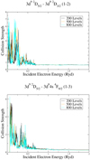 |
Fig. 2 Collision strengths for the 3d9 2D5∕2–3d9 2D3∕2 (1–2) and 3d9 2D5∕2–3d84s 4 F9∕2 (1–3) lines respectively, comparing the 200, 500 and 800 level calculations. |
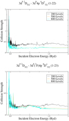 |
Fig. 3 Collision strengths for the 3d92D5∕2–3d84p4 D |


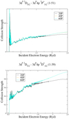 |
Fig. 4 Collision strengths for 20, 40, and 60 partial waves (PW) for the dipole transitions between the ground state 3d9 2D5∕2 and the 3d84p
2 P |


5 Ni II spectra
To illustrate the accuracy and usefulness of the data calculated in this paper, we construct a collisional-radiative model (Bates & McWhirter 1962) for Ni II using the effective collision strengths from the scattering calculation outlined in Sect. 4 and the radiative transition probabilities from the atomic structure calculations discussed in Sect. 2. A preliminary study is completed on the line spectra of Ni II using our collisional radiative code in order to show the potential applications for our data set. However, as our data set had been formatted for integration within the more powerful CLOUDY modelling programme (Ferland et al. 2017), there is an opportunity to undergo a more extensive modelling evaluation at a later date.
In order to form a collisional-radiative matrix Cjk we must balance the electron impact excitation and radiative decay rates. This allows the calculation of the photon emissivity coefficients (PECs) defined as,
 (14)
(14)
which is in units of number of photons cm−3.  is a reduced collisional-radiative matrix which has the ground state row removed. To further assess the accuracy of our data, we are initially looking at the 125–250 nm wavelength window. Figure 8 shows the shifted spectrum based upon Ni II, modelled using our scattering data using the colrad code (Bates & McWhirter 1962) to calculate the PEC’s. We highlight the observed lines from previous investigations. Good agreement for both strength and position is evident for well observed lines such as the 170.90 nm (Zsargó & Federman 1998; Fedchak et al. 2000; Fedchak & Lawler 1999) and 241.61 nm (Ferrero et al. 1997; Fedchak et al. 2000). Also, there is reasonable agreement for lesser observed lines such as the 131.72 nm line observed by Jenkins & Tripp 2006 theoretically predicted at a wavelength of 131.18 nm from our calculation. The unshifted spectrum results in a similar plot, except some of the smaller wavelengths are not in the correct positions, for example the 145.48 nm was at 150.22 nm. The intensity of the lines was also not as strong for the unshifted spectrum using this diagnostic line. In order to emphasise this strong diagnostic line we present in Fig. 9 the line ratio as a function of log electron temperature in K. We can clearly see that this line is heavily dependent on temperature, but has little dependence on density. The dashed lines on Fig. 9 indicate the upper and lower bounds of the unshifted model. The agreement between both models is good, which corresponds to the small percentage difference found between the two sets of data. Data of more interest for astrophysical modelling, is that pertaining to the florescent wavelength region witnessed in gaseous nebulae. The work by Bautista et al. (1996) discusses strong line ratios for the florescent line spectrum focused particularly on the spectrum observed in the Orion and Crab Nebulae. Other work which explores the florescent spectrum is the work of Lucy (1995), which investigates whether continuum florescence can account for the anomalous intensities observed in the spectra of many gaseous nebulae for particular lines of Ni II. Figure 10 presents the line spectrum of Ni II in the florescent wavelength region 650–750 nm for a density of 1 × 106 cm−3 and electron temperature of 3eV. Reasonable agreement is found with the position of the 737.8 and 741.2 nm lines discussed in both Bautista et al. (1996) and Lucy (1995) and found at 737.25 and 741.56 nm, respectively, using our modelling code. Good agreement is found with the 666.7 nm wavelength (Lucy 1995), seen in Fig. 10 at 666.69 nm.
6 Conclusion
The atomic data most reported in this paper represents the largest and most comprehensive dataset for electron impact excitation of Ni II currently available in the literature. Eleven configurations were included in the description of the target ion (Model 2) and the fully relativistic DARC R-Matrix package was employed in the collision calculations. Collision strengths were evaluated for all transitions, both forbidden and allowed, between the lowest 800 fine structure levels for incident electron energies up to 2 Ryd. We ensured that the Rydberg resonances converging onto the target state thresholds were properly resolved and the convergence of the high partial wave contributions was achieved. In order to access the accuracy of the collision strengths, two calculations were completed, a 149 jj level (Model 1) and a more substantial 800 jj level (Model 2). Furthermore, to investigate the effect of adjusting the energy levels during the collision calculation we have produced data sets with and without energy adjustments to enable us to clearly see the effect of such fine-tuning. The corresponding Maxwellian-averaged effective collision strengths were evaluated for a large range of electron temperatures log Te = 3.5–6.0 K, exceeding all other previous works. This data should provide the necessary quantity and quality of atomic data for modern day modelling of many astrophysical objects.
Comparisons were made with the earlier theoretical works of Cassidy et al. (2011) and Bautista (2004), where good agreement was found for many transitions. The exceptions were for those lines among split levels of the ground state at low temperatures, several intercombination lines which were significantly enhanced by high lying resonance features in the cross sections, and the high temperature region of the strong dipole lines. In addition, it was found that adjusting the energy levels to their NIST values did not significantly alter the results in either the 149 or 800 level evaluations.
Previous works (Ferrero et al. 1997; Fedchak & Lawler 1999; Fedchak et al. 2000; Zsargó & Federman 1998; Jenkins & Tripp 2006; Bautista et al. 1996; Lucy 1995) were used to compare with the Ni II spectrum modelled using our scattering data. Observed lines where identified between wavelengths of 125–250 nm and 650–750 nm, and show good agreement. There is an opportunity for more extensive modelling at a later stage using modelling programmes such as CLOUDY (Ferland et al. 2017).
The effective collision strengths produced from the present work shall be made available in adf04 format, along with the associated collision strengths via OPEN-ADAS website at https://open.adas.ac.uk.
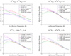 |
Fig. 5 Effective collision strengths for the 3d92 D5∕2–3d92 D3∕2(1–2), 3d92 D5∕2–3d84s4 F9∕2(1–3), 3d92 D5∕2–3d84s4 F7∕2(1–4) and 3d92 D5∕2–3d84s4 F5∕2(1–5) lines respectively. Comparisons are drawn with Cassidy et al. (2011) and Bautista (2004). Models are labelled by the number of levels the calculation contained. Model 1 is labelled as DARC149, and Model 2 is labelled as DARC800. |
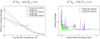 |
Fig. 6 Effective collision strengths between the ground state and the 3d84p4 D |

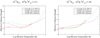 |
Fig. 7 Effective collision strengths for two dipole allowed transitions between the ground state to the 3d8 4p2 P |


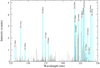 |
Fig. 8 Ni II spectrum presented for an electron temperature of 3 eV and electron density of 1 × 106 cm−3. The following highlighted lines correspond to transitions from the ground state 3d92 D5∕2
to 3d8 (1G)4p
2 F |


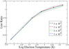 |
Fig. 9 Line ratio between the 170.96 nm, 3d92 D5∕2–3d84p2 F |


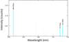 |
Fig. 10 Spectrum of Ni II for an electron temperature of 3 eV and electron density of 1 × 106 cm−3. The following highlighted lines correspond to transition lines of the forbidden multiplet 2F(a2 D-a2F). |
Acknowledgements
This work is supported by funding from the STFC ST/P000312/1 QUB Astronomy Observation and Theory Consolidated Grant. This work used the ARCHER UK National Supercomputing Service (http://www.archer.ac.uk), the Cray XC40 Hazel Hen supercomputer at HLRS Stuttgart under the PAMOP consortium. We wish to acknowledge the contributions of D. D. A. Clarke, A. T. Conroy, R. T. Smyth, and G. J. Ferland for their feedback when compiling this research.
References
- Ballance, C. P. 2019, DARC, http://connorb.freeshell.org [Google Scholar]
- Bates, David Robert, K. A. E., & McWhirter, R. W. P. 1962, 267 [Google Scholar]
- Bautista, M. A. 2004, A&A, 420, 763 [NASA ADS] [CrossRef] [EDP Sciences] [Google Scholar]
- Bautista, M. A., & Pradhan, A. K. 1996, A&AS, 115, 551 [NASA ADS] [Google Scholar]
- Bautista, M. A., Peng, J., & Pradhan, A. K. 1996, ApJ, 460, 372 [Google Scholar]
- Boissé, P., & Bergeron, J. 2019, A&A, 622, A140 [EDP Sciences] [Google Scholar]
- Burke, P. 2011, R-Matrix Theory of Atomic Collisions: Application to Atomic, Molecular and Optical Processes, Springer Series on Atomic, Optical, and Plasma Physics (Berlin: Springer Berlin Heidelberg) [Google Scholar]
- Cassidy, C. M., Ramsbottom, C. A., Scott, M. P., & Burke, P. G. 2010, A&A, 513, A55 [NASA ADS] [CrossRef] [EDP Sciences] [Google Scholar]
- Cassidy, C. M., Ramsbottom, C. A., & Scott, M. P. 2011, ApJ, 738, 5 [Google Scholar]
- Cassidy, C. M., Hibbert, A., & Ramsbottom, C. A. 2016, A&A, 587, A107 [NASA ADS] [CrossRef] [EDP Sciences] [Google Scholar]
- Cowan, R. D. 1981, The Theory of Atomic Structure and Spectra (California: University of California Press) [Google Scholar]
- Cucchiara, A., Cenko, S. B., Bloom, J. S., et al. 2011, ApJ, 743, 154 [Google Scholar]
- Davidson, K., Smith, N., Gull, T. R., Ishibashi, K., & Hillier, D. J. 2001, AJ, 121, 1569 [Google Scholar]
- Descouvemont, P., & Baye, D. 2010, Rep. Prog. Phys., 73, 036301 [Google Scholar]
- Dessauges-Zavadsky, M., Prochaska, J. X., D’Odorico, S., Calura, F., & Matteucci, F. 2006, A&A, 445, 93 [NASA ADS] [CrossRef] [EDP Sciences] [Google Scholar]
- Dyall, K., Grant, I., Johnson, C., Parpia, F., & Plummer, E. 1996, Comp. Phys. Comm., 94, 249 [Google Scholar]
- Fedchak, J. A., & Lawler, J. E. 1999, ApJ, 523, 734 [Google Scholar]
- Fedchak, J. A., Wiese, L. M., & Lawler, J. E. 2000, ApJ, 538, 773 [Google Scholar]
- Ferland, G. J., Chatzikos, M., Guzmán, F., et al. 2017, Rev. Mex. Astron. Astrofis., 53, 385 [NASA ADS] [Google Scholar]
- Fernandez, M. L., Smyth, R., Ramsbottom, C., & Ballance, C. 2019, MNRAS, 483, 2154 [Google Scholar]
- Ferrero, F. S., Manrique, J., Zwegers, M., & Campos, J. 1997, J. Phys. B At. Mol. Phys., 30, 893 [Google Scholar]
- Gruzdev, P. F. 1962, Opt. Spectr., 13, 249 [NASA ADS] [Google Scholar]
- Hibbert, A. 1975, Comput. Phys. Commun., 9, 141 [Google Scholar]
- Jenkins, E. B., & Tripp, T. M. 2006, ApJ, 637, 548 [Google Scholar]
- Klein, B., Jura, M., Koester, D., & Zuckerman, B. 2011, ApJ, 741, 64 [Google Scholar]
- Kramida, A., Ralchenko, Y., Reader, J., & NIST ASD Team 2019, NIST Atomic Spectra Database (version 5.5.6), https://physics.nist.gov/asd, online. Accessed: 2019-06-16 [Google Scholar]
- Kurucz, R. L. 2000, http://kurucz.harvard.edu/atoms.html [Google Scholar]
- Leighly, K. M., Halpern, J. P., Jenkins, E. B., & Casebeer, D. 2007, A&AS, 173, 1 [Google Scholar]
- Lucy, L. B. 1995, A&A, 294, 555 [NASA ADS] [Google Scholar]
- Mendlowitz, H. 1966, ApJ, 143, 573 [Google Scholar]
- Morton, D. C. 1991, ApJS, 77, 119 [Google Scholar]
- Nussbaumer, H., & Storey, P. J. 1982, A&A, 110, 295 [NASA ADS] [Google Scholar]
- Richardson, N. D., Gies, D. R., & Williams, S. J. 2011, AJ, 142, 201 [Google Scholar]
- Smyth, R., Johnson, C., Ennis, D., et al. 2017, Phys. Rev. A (At. Mol., Opt. Phys.), 96, 040303 [Google Scholar]
- Smyth, R., Ramsbottom, C., Keenan, F., Ferland, G., & Ballance, C. 2019, MNRAS, 483, 654 [Google Scholar]
- Véron-Cetty, M. P., Joly, M., Véron, P., et al. 2006, A&A, 451, 851 [NASA ADS] [CrossRef] [EDP Sciences] [Google Scholar]
- Watts, M. S. T., Berrington, K. A., Burke, P. G., & Burke, V. M. 1996, J. Phys. B At., Mol. Opt. Phys., 29, L505 [Google Scholar]
- Zsargó, J., & Federman, S. R. 1998, ApJ, 498, 256 [Google Scholar]
All Tables
Energy levels (Ryd) for the lowest lying 53 fine-structure states in Ni II obtained from Models 1 and 2.
Energy levels (Ryd) for the lowest lying 31 fine-structure states containing the 5s or 5p orbital for Ni II obtained from Model 2.
A coefficients (A-values in s −1) between the metastable levels from Model 2 compared with the data from Cassidy et al. (2016).
Einstein A coefficients (A-values in s −1) and absorption oscillator strengths (f-values in the length gauge) from Model 2 compared with the data from Cassidy et al. (2016) and Morton (1991).
Comparison of our fine-tuned oscillator strengths in the length gauge with the limited experimental determinations currently available.
Oscillator strengths of Ni II for transitions from the ground state to levels containing the 5p orbital and the ratio between the velocity and length gauge for the f-values.
All Figures
|
Fig. 1 Energy level spectrum of Ni II up to the 5p orbital, including the 4f orbital, organised by electronic configuration. Each horizontal line designates a specific fine structure level (taken from the NIST database). |
| In the text | |
|
Fig. 2 Collision strengths for the 3d9 2D5∕2–3d9 2D3∕2 (1–2) and 3d9 2D5∕2–3d84s 4 F9∕2 (1–3) lines respectively, comparing the 200, 500 and 800 level calculations. |
| In the text | |
|
Fig. 3 Collision strengths for the 3d92D5∕2–3d84p4 D |
| In the text | |
|
Fig. 4 Collision strengths for 20, 40, and 60 partial waves (PW) for the dipole transitions between the ground state 3d9 2D5∕2 and the 3d84p
2 P |
| In the text | |
|
Fig. 5 Effective collision strengths for the 3d92 D5∕2–3d92 D3∕2(1–2), 3d92 D5∕2–3d84s4 F9∕2(1–3), 3d92 D5∕2–3d84s4 F7∕2(1–4) and 3d92 D5∕2–3d84s4 F5∕2(1–5) lines respectively. Comparisons are drawn with Cassidy et al. (2011) and Bautista (2004). Models are labelled by the number of levels the calculation contained. Model 1 is labelled as DARC149, and Model 2 is labelled as DARC800. |
| In the text | |
|
Fig. 6 Effective collision strengths between the ground state and the 3d84p4 D |
| In the text | |
|
Fig. 7 Effective collision strengths for two dipole allowed transitions between the ground state to the 3d8 4p2 P |
| In the text | |
|
Fig. 8 Ni II spectrum presented for an electron temperature of 3 eV and electron density of 1 × 106 cm−3. The following highlighted lines correspond to transitions from the ground state 3d92 D5∕2
to 3d8 (1G)4p
2 F |
| In the text | |
|
Fig. 9 Line ratio between the 170.96 nm, 3d92 D5∕2–3d84p2 F |
| In the text | |
|
Fig. 10 Spectrum of Ni II for an electron temperature of 3 eV and electron density of 1 × 106 cm−3. The following highlighted lines correspond to transition lines of the forbidden multiplet 2F(a2 D-a2F). |
| In the text | |
Current usage metrics show cumulative count of Article Views (full-text article views including HTML views, PDF and ePub downloads, according to the available data) and Abstracts Views on Vision4Press platform.
Data correspond to usage on the plateform after 2015. The current usage metrics is available 48-96 hours after online publication and is updated daily on week days.
Initial download of the metrics may take a while.