| Issue |
A&A
Volume 647, March 2021
|
|
|---|---|---|
| Article Number | A184 | |
| Number of page(s) | 22 | |
| Section | Stellar structure and evolution | |
| DOI | https://doi.org/10.1051/0004-6361/202140289 | |
| Published online | 02 April 2021 | |
Mysterious, variable, and extremely hot: White dwarfs showing ultra-high excitation lines
I. Photometric variability
1
Institute for Physics and Astronomy, University of Potsdam, Karl-Liebknecht-Str. 24/25, 14476 Potsdam, Germany
e-mail: This email address is being protected from spambots. You need JavaScript enabled to view it.
2
Department of Physics, University of Warwick, Cosventry CV4 7AL, UK
3
Instituto de Física, Universidade Federal do Rio Grande do Sul, 91501-900 Porto-Alegre, RS, Brazil
Received:
6
January
2021
Accepted:
3
February
2021
Abstract
Context. About 10% of all stars exhibit absorption lines of ultra-highly excited (UHE) metals (e.g., O VIII) in their optical spectra when entering the white dwarf cooling sequence. This is something that has never been observed in any other astrophysical object, and poses a decades-long mystery in our understanding of the late stages of stellar evolution. The recent discovery of a UHE white dwarf that is both spectroscopically and photometrically variable led to the speculation that the UHE lines might be created in a shock-heated circumstellar magnetosphere.
Aims. We aim to gain a better understanding of these mysterious objects by studying the photometric variability of the whole population of UHE white dwarfs, and white dwarfs showing only the He II line problem, as both phenomena are believed to be connected.
Methods. We investigate (multi-band) light curves from several ground- and space-based surveys of all 16 currently known UHE white dwarfs (including one newly discovered) and eight white dwarfs that show only the He II line problem.
Results. We find that 75−13+8% of the UHE white dwarfs, and 75−19+9% of the He II line problem white dwarfs are significantly photometrically variable, with periods ranging from 0.22 d to 2.93 d and amplitudes from a few tenths to a few hundredths of a magnitude. The high variability rate is in stark contrast to the variability rate amongst normal hot white dwarfs (we find 9−2+4%), marking UHE and He II line problem white dwarfs as a new class of variable stars. The period distribution of our sample agrees with both the orbital period distribution of post-common-envelope binaries and the rotational period distribution of magnetic white dwarfs if we assume that the objects in our sample will spin-up as a consequence of further contraction.
Conclusions. We find further evidence that UHE and He II line problem white dwarfs are indeed related, as concluded from their overlap in the Gaia HRD, similar photometric variability rates, light-curve shapes and amplitudes, and period distributions. The lack of increasing photometric amplitudes towards longer wavelengths, as well as the nondetection of optical emission lines arising from the highly irradiated face of a hypothetical secondary in the optical spectra of our stars, makes it seem unlikely that an irradiated late-type companion is the origin of the photometric variability. Instead, we believe that spots on the surfaces of these stars and/or geometrical effects of circumstellar material might be responsible.
Key words: white dwarfs / stars: variables: general / starspots / binaries: close
© ESO 2021
1. Introduction
White dwarfs are the end products of the vast majority of all stars, with about 20% of them being H-deficient. They are observed over a huge temperature interval, ranging from 250 000 K (Werner & Rauch 2015) down to 2710 K (Gianninas et al. 2015). The early stages of white dwarf cooling occur very rapidly. When a star enters the white dwarf cooling sequence, it cools down to 65 000 K within less than a million years, while the cooling phase down to 3000 K takes several billion years (Althaus et al. 2009; Renedo et al. 2010). Thus, although about 37 000 white dwarfs have been spectroscopically confirmed (Kepler et al. 2019), only a tiny fraction (< 1%) have effective temperatures (Teff) above 65 000 K.
These extremely hot white dwarfs cover a large but sparsely populated region in the Hertzsprung-Russell Diagram (HRD) and represent an important link in stellar evolution between the (post-)asymptotic giant branch (AGB) stars, and the bulk of the white dwarfs on the cooling sequence. Several intriguing physical processes take place during the early stages of white dwarf cooling that mark those stars as important astronomical tools even beyond stellar evolution studies. The intense extreme ultraviolet (UV) radiation from a very hot white dwarf can evaporate giant planets. A fraction of the evaporated volatiles may then be accreted, polluting the atmosphere of the white dwarf (Gänsicke et al. 2019; Schreiber et al. 2019). Therefore, detailed abundance analyses of hot white dwarfs can provide information on the potential of these objects to reconstruct the composition of exosolar gaseous planets. Some white dwarfs in the Teff interval 58 000 − 85 000 K were found to display high abundances of trans-iron group elements (atomic number Z > 29), which is thought to be caused by efficient radiative levitation of those elements (Chayer et al. 2005; Hoyer et al. 2017, 2018; Löbling et al. 2020). These stars serve as important stellar laboratories to derive atomic data for highly ionized species of trans-iron elements (Rauch et al. 2012, 2014a,b, 2015a,b, 2016, 2017a,b). Hot white dwarfs have also proven to be powerful tools for Galactic archaeology and cosmology. They are employed to check a dependency of fundamental constants, for example the fine structure constant α, with gravity (Berengut et al. 2013; Bainbridge et al. 2017; Hu et al. 2021), to derive the age of the Galactic halo (Kalirai 2012; Kilic et al. 2019) or to derive the properties of weakly interacting particles via the hot white dwarf luminosity function (Isern et al. 2008; Miller Bertolami 2014; Miller Bertolami et al. 2014).
A particularly baffling phenomenon that takes place at the beginning of the white dwarf cooling sequence is the presence of (partly very strong) absorption lines of ultra-highly excited (UHE) metals (e.g., N VII, O VIII) in the optical spectra of the hottest white dwarfs. The occurrence of these obscure features requires a dense environment with temperatures of the order 106 K, by far exceeding the stellar effective temperature. A photospheric origin can therefore be ruled out. As some of the UHE lines often exhibit an asymmetric profile shape, it was first suggested that those lines might form in a hot, optically thick stellar wind (Werner et al. 1995). Another peculiarity of these objects is that all of them show the Balmer or He II line problem, meaning that their Balmer/He II lines are unusually deep and broad and cannot be fitted with any model. There are also white dwarfs showing only the Balmer/He II line problem, but no UHE lines. Regarding the H-rich (DA-type) white dwarfs, it was found that the Balmer line problem is to some extent due to the neglect of metal opacities in the models (Werner 1996). But there are also cases in which the Balmer line problem persists, even when sophisticated models are used (Gianninas et al. 2011; Werner et al. 2018a, 2019). However, for the He-dominated (DO-type) white dwarfs showing the He II line problem, even the addition of metal opacities to the models does not help to overcome this problem. As the He II line problem is observed in every UHE white dwarf – without exception –, a link between these two phenomena seems very likely (Werner et al. 2004). It is thought that the “He II line problem” objects are related to the UHE white dwarfs and that the same process is operating in these stars but is failing to generate the UHE features (Werner et al. 2014).
The Balmer/He II line problem also makes it difficult – if not impossible – to derive accurate temperatures, gravities, and spectroscopic masses. Some objects show weak He I lines that allow to constrain their Teff to some degree. High-resolution UV spectroscopy is available only for three UHE white dwarfs, which were analyzed by Werner et al. (2018b). These latter authors found that the Teff derived by exploiting several ionization balances of UV metal lines agree with what can be estimated from the He I/He II ionization equilibrium in the optical. In addition, the study revealed that light metals (C, N, O, Si, P, and S) are found in these objects at generally subsolar abundances and heavy elements from the iron group (Cr, Mn, Fe, Co, Ni) with solar or supersolar abundances. This is not different from other hot white dwarfs and can be understood as a result of gravitational settling and radiative levitation of elements. Werner et al. (2018b) discussed the possibility that the UHE lines might form in a multicomponent radiatively driven wind that is frictionally heated. Such winds are expected to occur in a narrow strip in the Teff − log g-diagram (Fig. 4 in Krtička & Kubát 2005), which indeed overlaps with the region in which the UHE white dwarfs are observed (see Fig. 3 in Reindl et al. 2014).
While this strip could explain why the occurrence of UHE features is restricted to white dwarfs hotter than ≈65 000 K, the model does not explain why not all hot white dwarfs located in this region show this phenomenon. In addition, the frictionally heated wind model, which assumes a spherically symmetric wind, fails to explain the photometric and spectroscopic variability of the UHE white dwarf J01463+3236 discovered by Reindl et al. (2019). These latter authors reported for the first time rapid changes of the equivalent widths (EWs) of the UHE features in the spectra of J01463+3236, which were found to be correlated to the photometric period of the star (≈0.24 d). Interpreting this period as the rotational period of the star, they argue that the UHE features are rotationally modulated and stem from a co-rotating, shock-heated, circumstellar magnetosphere. Furthermore, they suggested that the cooler parts of the magnetosphere likely constitute an additional line-forming region of the overly broad and overly deep He II lines (or Balmer lines in the case of DAs). White dwarfs that lack the UHE lines and only show the Balmer/He II line problem could then be explained by having cooler magnetospheres with temperatures not high enough to produce UHE lines. As this model requires the white dwarfs to be at least weakly magnetic (meaning that they should have magnetic field strengths above a few hundred to a thousand Gauss), it could also explain why only a fraction of the hottest white dwarfs show UHE lines.
The UHE phenomenon affects about 10% of all stars in the universe when entering the white dwarf cooling sequence, and therefore a better understanding of these objects is highly desirable. Here, we aim to study the properties of the UHE white dwarfs, as well as their relatives – white dwarfs showing only the He II line problem – as a whole. In particular, we want to find out whether or not the photometric and spectroscopic variability observed in J0146+3236 is something that affects all UHE white dwarfs, and possibly also the He II line problem white dwarfs. This article is the first in a series of papers and introduces the sample of UHE and He II line problem white dwarfs and investigates their photometric variability. In Sect. 2 we first present the sample and discuss the location of these stars in the Gaia HRD. We then present our search for photometric variability using light curves from various ground- and space-based surveys (Sect. 3). The overall results of this study are presented in Sect. 4. Finally, we discuss our findings (Sect. 5) and provide an outlook on how more progress can be made (Sect. 6).
2. The sample of UHE and He II line problem white dwarfs
The first two UHE white dwarfs, the DO-type white dwarfs HS 0713+3958 and HE 0504−2408, were discovered by Werner et al. (1995). Soon afterwards, Dreizler et al. (1995) announced a further three DO-type UHE white dwarfs (HS 0158+2335, HS 0727+6003, and HS 2027+0651) as well as the first H-rich UHE white dwarf (HS 2115+1148), which they found in the Hamburg-Schmidt (HS) survey (Hagen et al. 1995). The number of UHE white dwarfs increased even further with the Sloan Digital Sky Survey (SDSS). Hügelmeyer et al. (2006) reported two DO-type UHE white dwarfs and one DOZ (PG 1159) UHE white dwarf from the SDSS DR4. Within the SDSS DR10, two more DO-type UHE white dwarfs were found (Werner et al. 2014; Reindl et al. 2014), and Kepler et al. (2019) announced the discovery of two more DA-type UHE white dwarfs as well as one (or possibly two) more DO-type UHE white dwarf within the SDSS DR14. One more DO-type UHE white dwarf was discovered by Reindl et al. (2019) based on spectroscopic follow-up of UV-bright sources. Finally, we announce the discovery of a sixteenth member of the UHE white dwarfs, the DOZ-type WD 0101−182. In archival UVES spectra of this star (R ≈ 18 500, ProgID 167.D-0407(A), PI: R. Napiwotzki), we detect for the first time UHE lines around 3872, 4330, 4655, 4785, 5243, 5280, 6060, 6477 Å (Fig. B.1). Using nonlocal thermodynamic equilibrium (NLTE) models for DO-type white dwarfs (Reindl et al. 2014, 2018) that were calculated with the Tübingen NLTE Model-Atmosphere Package (TMAP, Werner et al. 2003, 2012), we find that the weak He Iλ5876 Å line and the C IVλ5803, 5814 Å doublet are best reproduced with Teff = 90 000 K and C = 0.003 (mass fraction).
In addition to these 16 UHE white dwarfs, our sample includes eight more objects that show only the He II line problem but no clear sign of UHE lines. The prototype of this class of stars is HE 1314+0018, which was discovered by Werner et al. (2004). The high-resolution and high-signal-to-noise spectrum of HE 1314+0018 lacks any UHE absorption lines. The other seven objects are from the samples of Dreizler & Heber (1998), Werner et al. (2014), and Kepler et al. (2019). Four of them possibly show the UHE feature around 5430−5480 Å, which is also one of the strongest UHE features observed in the UHE white dwarfs.
In Figs. B.1 and B.2 we show the optical spectra of all UHE white dwarfs and spectra of all white dwarfs showing only the He II line problem, respectively. For HS 2027+0651, HST/STIS spectra are shown that were observed with the G430L and G750L gratings (R ≈ 700). We downloaded these observations from the Mikulski Archive for Space Telescopes (MAST, proposal IDs: 8422, 7809, PIs: H. Ferguson and C. Leitherer, respectively). For WD 0101–182, the UVES spectrum (see above), and for HE 0504–2408 an EFOSC 1 spectrum obtained at the ESO 3.6 m telescope (R ≈ 1500, Werner et al. 1995) are shown. The spectra of J0146+3236, HS 0158+2335, HS 0713+3958, HS 0727+6003, HS 0742+6520, and HE 1314+0018 were obtained by us in October and November 2014 at the Calar Alto 3.5 m telescope (ProgID H14-3.5-022, see also Reindl et al. 2019). We used the TWIN spectrograph and a slit width of 1.2 acrsec. For the blue channel grating No. T08, and for the red channel grating No. T04 were used. The spectra have a resolution of 1.8 Å. After each spectrum, we required ThAr wavelength calibration. Data were reduced using IRAF. We did not flux-calibrate our data. For HS 1517+7403 and HS 2115+1148, TWIN spectra are shown that were obtained by Dreizler et al. (1995) and Dreizler & Heber (1998) and have a resolution of 3.5 Å. For the remaining objects, SDSS spectra (R ≈ 1800) are shown. Overplotted in red are TMAP models with atmospheric parameters determined within this work (WD 0101−182) or with parameters reported by previous works (see footnote of Table 1).
Names, spectral types, J2000 coordinates, observed Gaia eDR3 G band magnitudes, distances, Gaia extinction coefficients, dereddened Gaia color indexes, and the absolute dereddened G band magnitudes of all known UHE white dwarfs and white dwarfs showing only the He II line problem.
Table 1 lists all UHE and He II line problem white dwarfs along with their spectral types, J2000 coordinates, observed Gaia early DR3 G band magnitudes (Gaia Collaboration 2016, 2018), distances, d, Gaia extinction coefficients, AG, the dereddened Gaia color indexes, (BP − RP)0, and the absolute dereddened G band magnitudes. A spectral type DOZ UHE indicates a He-rich white dwarf that shows photospheric metal lines in the optical as well as UHE lines. A spectral subtype ‘UHE’: indicates an object with an uncertain identification of UHE lines. We calculated distances from the parallaxes (via 1000/π), which we corrected for the zeropoint bias using the Python code provided by Lindegren et al. (2021)1. Following Gentile Fusillo et al. (2019), we assume that the extinction coefficient AG in the GaiaG passband scales as 0.835 × AV based on the nominal wavelengths of the respective filters and the reddening versus wavelength dependence employed by Schlafly & Finkbeiner (2011). Values for AV were obtained from the 3D dust map of Lallement et al. (2018) using the distance calculated from the Gaia parallax of each object. Nine of our stars are located outside of the Lallement et al. (2018) 3D dust map (that is stars with a distance from the Galactic plane of |z| ≳ 500 pc). For those, we obtained AV from the 2D dust map of Schlafly & Finkbeiner (2011) and assumed that AG scales with a factor of 1 − exp(−|z|/200 pc), as most of the absorbing material along the line of sight is concentrated along the plane of the Galactic disk. We note that the difference in reddening obtained from the two methods varies by a factor of 0.65 to 2.24 for stars located within the 3D dust map (−500 pc < z < 500 pc). This demonstrates that an accurate determination is not easy. The color indices, (BP − RP)0, were calculated using Eqs. (18) and (19) in Gentile Fusillo et al. (2019). The absolute Gaia magnitude in the G band was calculated via MG0 = G − AG + 5 + 5 × log(π/1000), where π is the zero-point-corrected parallax in milliarcseconds from the Gaia early DR3.
Figure 1 shows the locations of the UHE white dwarfs (star symbols) and white dwarfs showing only the He II line problem (diamonds) that have parallaxes better than 20% in the Gaia HRD. Also shown are the locations of white dwarfs from the SDSS (dots) with Gaia parallaxes better than 5% and a reddening smaller than EB − V < 0.015 (Gaia Collaboration 2018), as well as hot subdwarfs (triangles) from Geier (2020) with Gaia parallaxes better than 20%. The latter were dereddened following the approach of Gentile Fusillo et al. (2019). Finally, we also show the locations of white dwarf-main sequence binaries (bold plus signs) from the sample of Rebassa-Mansergas et al. (2010) that contain a very hot (Teff ≥ 50 000 K) white dwarf primary and have parallaxes better than 30%.
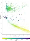 |
Fig. 1. Locations of the UHE white dwarfs (star symbols) and white dwarfs showing only the He II line problem (diamonds) in the Gaia HRD. Hot subdwarfs (triangles), SDSS white dwarfs (dots), and white dwarf–main sequence binaries (plus symbols) containing a very hot (Teff ≥ 50 000 K) white dwarf are also shown. The color coding indicates the effective temperatures of the stars. |
It can be seen that the UHE white dwarfs and white dwarfs showing only the He II line problem overlap in a narrow region (−0.71 mag ≤ (BP − RP)0 ≤ −0.37 mag, and 7.19 mag ≤ MG ≤ 8.43 mag). Both are located well below the hot subdwarf cloud and are just on top of the white dwarf banana2. It also becomes clear that the stars in our sample are amongst the bluest objects. Most of the hot white dwarfs with an M-type companion are found at similar absolute magnitudes, but redder colors. This is a consequence of the flux of the low-mass companion that significantly contributes to the flux in the optical wavelength range. The only object from the sample of Rebassa-Mansergas et al. (2010) that lies directly on the white dwarf banana is SDSS J033622.01–000146.7. For this object, the late-type companion is not noticeable in the continuum flux (no increased flux at longer wavelengths) and also shows no absorption lines from the secondary. Only the emission lines in the core of the Balmer series are seen, which originate from the close and highly irradiated side of the cool companion. Two of our stars, the DA-type UHE white dwarf J1257+4220 and J0827+5858, which shows only the He II line problem, are found at noticeably redder colors (−0.42 mag and −0.37 mag, respectively) than the rest of our sample. While J0827+5858 is located at a region with a particularly high reddening Ag = 0.32 mag, which might be underestimated by the 3D dust map, this is unlikely the case for J1257+4220 (AG = 0.04 mag). Looking at the Gaia eDR3 Renormalized Unit Weight Error (RUWE) values of our stars, we find they all have a value close to one (indicating that the single-star model provides a good fit to the astrometric observations), except for J1257+4220. Here we find a RUWE value much larger than one, namely 1.3387. This might suggest that J1257+4220 is a (wide) binary or it was otherwise problematic for the astrometric solution.
The mean dereddend color index of our sample is  mag (standard deviation σ = −0.08 mag), with the UHE white dwarfs being slightly bluer (
 mag, σ = −0.07 mag) than white dwarfs showing only the He II line problem (
 mag, σ = −0.08 mag). We also find that the mean dereddened absolute G band magnitude of the UHE white dwarfs with parallaxes better than 20% (
 mag, σ = −0.27 mag) is slightly brighter than that of white dwarfs showing only the He II line problem (
 mag, σ = −0.56 mag).
We note that 18 out of the 24 stars in our sample have a probability of being a white dwarf (PWD) of greater than 90% as defined by Gentile Fusillo et al. (2019). For the remaining objects, we find PWDs between 72% and 89%. The only object that is not included in the catalog of Gentile Fusillo et al. (2019) is J0900+2343, which is also the only object in our sample that has a negative parallax in the Gaia DR2. For comparison, the catalog of hot subdwarf candidates from the Gaia DR2 by Geier et al. (2019) contains only three of our stars. This is because for objects with parallaxes better than 20%, Geier et al. (2019) included only objects with absolute magnitudes in the range −1.0 mag ≤ MG ≤ 7.0 mag.
3. Light-curve analysis
The discovery of photometric variability in the UHE white dwarf J01463+3236 raises the question of whether photometric variability is a common feature of UHE white dwarfs, and possibly also of the He II line problem white dwarfs. Here we want to investigate this possibility by searching for periodic signals in the light curves of these objects.
For the analyses of the light curves, we used the VARTOOLS program (Hartman & Bakos 2016) to perform a generalized Lomb-Scargle (LS) search (Zechmeister & Kürster 2009; Press et al. 1992) for periodic sinusoidal signals. We classify objects that show a periodic signal with a false alarm probability (FAP) of log(FAP)≤ − 4 as significantly variable, objects with −3 ≤ log(FAP) < − 4 as possibly variable, and objects that only show a periodic signal with log(FAP) > − 3 as not variable. In cases where we found more than one significant period, we whitened the light curve by removing the strongest periodic signal (including its harmonics and subharmonics) from the light curve. The periodogram was then recomputed to check whether or not the FAP of the next strongest signal still remains above our variability threshold (log(FAP)≤ − 4). This whitening procedure was repeated until no more significant periodic signals could be found.
Using the -killharm command we fitted a harmonic series of the form
 (1)
(1)
to each light curve. We use this to determine the peak-to-peak amplitude of the light curve, which we define as the difference between the maximum and minimum of the fit. The same function was also used to estimate the uncertainties on the derived periods by running a Differential Evolution Markov chain Monte Carlo (DEMCMC) routine (Ter Braak 2006) employing the –nonlinfit command. The number of accepted links was set to 10 000. As initial guesses we used the period obtained from the LS search, and for the remaining parameters the values from the killharm fit.
In Tables A.1 and A.2, we summarize the light curves used in our analysis, the data points of each light curve, the mean magnitude in each band, the median value of each period and its uncertainty as calculated in the DEMCMC simulation, and amplitudes for the UHE white dwarfs and white dwarfs showing only the He II line problem, respectively. In the following, we provide an overview of the data sets used in our work (Sect. 3.1) and then provide notes on individual objects (Sect. 3.2).
3.1. Data sets
Light curves were obtained from various surveys as well as our own observing campaign.
TESS. The Transiting Exoplanet Survey Satellite (TESS) scans the sky with 26 segments and with a 27.4 day observing period per segment. TESS uses a red-optical bandpass covering the wavelength range from about 6000 to 10 000 Å centered on 7865 Å, as in the traditional Cousins I-band. We downloaded the target pixel files (TPF) of each object from MAST as FITS format. The FITS files are already processed based on the Pre-Search Data Conditioning Pipeline (Jenkins et al. 2016) from which we extracted the barycentric corrected dynamical Julian days (“BJD – 2457000”, a time system that is corrected by leap seconds; see Eastman et al. 2010) and the pre-search Data Conditioning Simple Aperture Photometry flux (“PDCSAP FLUX”) for which long-term trends have been removed using the co-trending basis vectors. In this work, we used the PDC light curves and converted the fluxes to fractional variations from the mean (i.e., differential intensity). As TESS has a poor spatial resolution (one detector pixel corresponds to 21 arcsec on the sky) and our targets are faint, we carefully checked for blends with close-by stars using the tpfplotter code (Aller et al. 2020). In Fig. 2 we show the TPF plots for the UHE and He II line problem white dwarfs. The red circles represent Gaia sources, which are scaled by magnitude contrast against the target source. Also shown is the aperture mask used by the pipeline to extract the photometry. In total, ten UHE, and two He II problem white dwarfs were observed by TESS in the two-minute cadence mode.
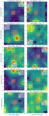 |
Fig. 2. From left to right and top to bottom: target pixel files (TPFs) of WD 0101−182, J0146+3236, HS 0158+2335, J0254+0058, HS 0713+3958, HS 0727+6003, HS 0742+6520, HE 1314+0018, J1510+6106, and HS 1517+7403. The red circles are the sources of the Gaia catalog in the field with scaled magnitudes (see legend). Number 1 indicates the location of the targets. The aperture mask used by the pipeline to extract the photometry is also marked. |
K2. In a series of sequential observing campaigns, 20 fields, which were distributed around the ecliptic plane, were observed by the K2 mission (campaign duration ≈80 d, Howell et al. 2014). Throughout the mission, K2 observed in two cadence modes: long cadence (≈30 min data-point cadence) and short cadence (≈1 min data-point cadence). The latter was only provided for selected targets, and the long cadence was used as the default observing mode. Two of the stars in our sample, J0821+1739 and J0900+2343, were observed in long-cadence mode. K2 data contain larger systematic errors than the original Kepler mission. This is because of the reduction in pointing precision as a result of the spacecraft drift during the mission. Thus, several pipelines have been developed to process K2 light curves. Here, we are using the light curves produced by the K2 Self Flat Fielding (K2SFF, Vanderburg & Johnson 2014) and the EPIC Variability Extraction and Removal for Exoplanet Science Targets (EVEREST, Luger et al. 2016, 2018) pipelines. The data were obtained from the MAST archive.
ATLAS. Since 2015, the Asteroid Terrestrial-impact Last Alert System (ATLAS, Tonry et al. 2018) has been surveying approximately 13 000 deg2 at least four times per night using two independent and fully robotic 0.5 m telescopes located at Haleakala and Mauna Loa in Hawaii. It provides c- and o-band light curves (effective wavelengths 0.53 μm and 0.68 μm, respectively) which are taken with an exposure time of 30 s. Eight stars in our sample have ATLAS light curves.
Catalina Sky Survey. The Catalina Sky Survey uses three 1 m class telescopes to cover the sky in the declination range −75° < δ < +65°, but avoids the crowded Galactic plane region by 10−15° due to reduced source recovery. It consists of the Catalina Schmidt Survey (CSS), the Mount Lemmon Survey (MLS) in Tucson, Arizona, and the Siding Spring Survey (SSS) in Siding Spring, Australia. The second data release contains V-band photometry for about 500 million objects with V magnitudes between 11.5 and 21.5 from an area of 33 000 sq. deg. (Drake et al. 2009, 2014). Most of the stars in our sample are covered by this survey, though we find that at least 200−300 data points are needed to find a periodic signal. This is likely because of the larger uncertainties on the photometric measurements compared to other surveys employed in this work.
SDSS stripe 82. The SDSS Stripe 82 covers an area of 300 deg2 on the celestial equator, and has been repeatedly scanned in the u-, g-, r-, i-, and z-bands by the SDSS imaging survey (Abazajian et al. 2009). For J0254+0058, the only object in our sample that is included in the SDSS stripe 82, we acquired the u-, g-, r-, i-, and z-band light curves (about 70 data points each) from Ivezić et al. (2007).
ZTF. The Zwicky Transient Facility (ZTF, Bellm et al. 2019; Masci et al. 2019) survey uses a 48-inch Schmidt telescope with a 47 deg2 field of view, which ensures that the ZTF can scan the entire northern sky every night. We obtained data from the DR4 which were acquired between March 2018 and September 2020, covering a time-span of around 470 days. The photometry is provided in the g and r bands, and also in the i-band but with less frequency, with a uniform exposure time of 30 s per observation. Most objects in our sample are covered by this survey, with 21 having at least 50 data points in at least one band.
BUSCA. For HS 0727+6003 we obtained photometry using the Bonn University Simultaneous Camera (BUSCA, Reif et al. 1999) at the 2.2 m telescope at the Calar Alto Observatory. The star was observed during two consecutive nights on 21 and 22 December 2018. The beam splitters of BUSCA allow visible light to be collected simultaneously in four different bands, namely UB, BB, RB, and IB. However, due to technical problems with BUSCA, we were not able to obtain data in IB band. Instead of filters, we used the intrinsic transmission curve given by the beam splitters to avoid light loss. We used the IRAF aperture photometry package to reduce the data.
3.2. Notes on individual objects
3.2.1. UHE white dwarfs
J0032+1604. This object is a DO-type UHE white dwarf with the strongest UHE features seen in any of the objects discussed here. It was observed within CSS and ATLAS. The periodograms of all light curves show the strongest signal around 0.91 d. Heinze et al. (2018) reported twice the period (P = 1.81619 d). The amplitude of the light curve variations ranges from 0.05 mag to 0.07 mag, but is not found to differ significantly. In the first two rows on the left side of Fig. 3, we show the periodogram and phase-folded light curve from the ATLAS c-band, which predicts lowest FAP. The original periodogram is shown in gray and the whitened periodogram is shown in light blue. No other significant signal is left after whitening the light curve for the 0.91 d periodicity. The black line on top of the phase-folded light curve (red) is a fit of a harmonic series used to predict the peak-to-peak amplitude.
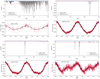 |
Fig. 3. Periodograms and phase-folded light curves of the UHE white dwarfs J0032+1604, WD 0101−182, J0146+3236, and HS 0158+2335. The red solid lines are phase-averaged light curves, while the dotted light curve represents the actual data. The black line is a fit of a harmonic series used to predict the peak-to-peak amplitude. |
WD0101−182. This bright (G = 15.74 mag) DOZ-type UHE white dwarf was observed with TESS, CSS, and ATLAS. The periodogram of the TESS light curve shows the strongest peak around 2.32 d. This period is also confirmed by the CSS V band and ATLAS c band light curves, respectively. The periodogram of the ATLAS o-band light curve predicts the strongest peak at 1.747674 d, but another significant peak occurs at 2.31 d, close to what is found in the ATLAS c, CSS V, and TESS band. We also note that the 2.32 d periodicity is already clearly visible in the unfolded TESS light curve and is also reported by Heinze et al. (2018). The amplitudes of the ATLAS and CSS phase-folded light curves are consistent.
J0146+3236. This is the only object for which rapid changes in the EW of the UHE features have been observed. Drake et al. (2014) and Heinze et al. (2018) reported photometric variability of P = 0.484074 d (based on CSS data) and P = 0.48408 d (based on ATLAS data), respectively, while Reindl et al. (2019) reported half of that value. We can confirm the period found by Reindl et al. (2019) based on ATLAS, ZTF, and TESS data. The periodogram of the TESS light curve shows the strongest signal at P = 0.242037 d. All other significant peaks turned out to be (sub-)harmonics of this period (Fig. 3). The shape of the phase-folded light curves is roughly sinusoidal, with extended flat minima.
HS 0158+2335. This object was observed with CSS, ATLAS, ZTF, and TESS. In the TESS light curve, we detect the strongest signal around 0.45 d. No other significant period is left after the first whitening cycle. In the periodograms calculated for the ATLAS o-band (96 data points) and ZTF g-band (43 data points) no significant periodic signal can be detected. In all other light curves we also find a significant period at P ≈ 0.45 d. The period found by us is confirmed by Drake et al. (2014) who reported P = 0.449772 d based on CSS DR 1 data. Heinze et al. (2018), on the other hand, reported twice the period (P = 0.899571 d) found by us. The shape of the phase-folded light curves clearly shows two maxima, with the first one being at phase 0.0, and the second at approximately phase 0.6, and the minimum is located around phase 0.3.
J0254+0058. This object was observed within CSS, ATLAS, ZTF, and TESS, and is the only object in our sample included in the SDSS stripe 82 survey. Becker et al. (2011), Drake et al. (2014), and Heinze et al. (2018) report a period of about 2.17 d for this object based on SDSS stripe 82 (u, g, and r band), CSS V band, and ATLAS o- and c-band light curves, respectively. The periodograms of the light curves of all surveys mentioned above predict the strongest periodic signal at around 1.09 d. The amplitudes of the phase-folded light curves are always around 0.3 mag and do not differ significantly amongst the different bands. The shapes of the phase-folded light curves are, as in J0146+3236, roughly sinusoidal, with broad and flat minima (top row left in Fig. 4). After whitening the TESS light curve for the 1.09 d periodic signal and its (sub-)harmonics, we find one more significant peak around 1.3 d (marked with an “x” in Fig. 4) just above our variability threshold (log(FAP) = − 4.4 < −4). After the second whitening cycle, no other significant peak is left in the periodogram.
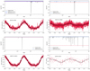 |
Fig. 4. As in Fig. 3 for the UHE white dwarfs J0254+0058, HS 0713+3958, HS 0727+6003, and J1059+4043. |
HE 0504−2408 is one of the objects showing the strongest UHE features, and one of the brightest (G = 15.77 mag) stars in our sample. It was observed in the course of the CSS (69 data points) and the SSS (182 data points). The SSS light curve indicates that the star underwent a brightening of 0.4 mag from MJD = 53599 to MJD = 53755 and remained at V ≈ 15.65 mag. Using only data obtained after MJD = 53755 we find a period of 0.684304 d with an associated log(FAP) = − 3.4. The amplitude of the phase-folded light curve is 0.08 mag, and its shape is sinusoidal. We classify this star as possibly variable.
HS 0713+3958. This object is yet another example where the phase-folded light curve shows extended, flat minima (second row right in Fig. 4). The periodogram of the TESS light curve shows the strongest periodic signal around P = 0.78 d (first row right in Fig. 4). No other significant signal is left in the periodogram after whitening the light curve for this periodicity. The strongest periodic signals in the CSS and ZTF g- and r-band light curves are also detected around 0.78 d. In the ATLAS c- and o-band light curve, the strongest periodic signals are found at 1.379916 d and 0.304796 d, respectively. However, we also find periodic signals around 0.78 d above our FAP threshold in both periodograms. Heinze et al. (2018) report a period of P = 0.609618 d, which is twice what we found as the strongest signal in the ATLAS o-band. We adopt the 0.781646 d period from the TESS light curve.
Ground-based infrared photometry by Napiwotzki (1997) revealed a nearby star to HS 0713+3958. Werner et al. (2018a), who recorded an optical spectrum with the Hubble Space Telescope (HST) of this late-type star, determined a spectral type of M5V and found that the spectroscopic distances of both stars agree within the error limits. Comparing the fluxes of the HST spectrum of the M5V star with the SDSS spectrum, we find that the flux of the cool star only dominates beyond 10 000 Å, which is beyond the TESS filter pass band. This implies that the periodicity found in our light curve analysis most likely originates from the hot white dwarf and not from the cool star. Another interesting fact is that companions of spectral type M5 or later may easily be hidden in the optical due to the still high luminosity of the white dwarf. We also note that Gaia clearly resolved the white dwarf and the M5 star (we calculate a separation of 1.0396 ± 0.0005 arcsec), and therefore it is not possible that the two stars form a close binary.
HS 0727+6003. The periodogram of the TESS light curve for this object shows the strongest periodic signal around P = 0.22 d (penultimate row right in Fig. 4). No other significant period is found after the first whitening cycle. The ≈0.22 d period is also found in the CSS, ATLAS c- and o-band, and ZTF g- and r-band light curves. Again, the minima of the phase-folded light curves are broad and flat. The amplitudes are all around 0.13 mag and do not differ significantly amongst the different bands. Drake et al. (2014) gives a period of P = 0.28437 d, higher than what we find. Heinze et al. (2018) reports twice our period (P = 0.442823 d). With BUSCA we were able to record almost two phases, and find that the amplitudes of the UB, BB, and RB band light curves (0.128 ± 0.014 mag, 0.131 ± 0.008 mag, and 0.128 ± 0.011 mag, respectively) agree with each other as well as with the amplitudes from the light curves from the other surveys.
HS 0742+6520. Like HE 0504−2408, this object shows some of the strongest UHE features and is found to be not significantly variable. It was observed only 121 times in the course of the CSS. The TESS light curve predicts the strongest peak at 0.281989 d with an associated log(FAP) = − 1.7. The phase-folded light curve has an amplitude of 0.01 mag only. Thus, this star is likely not variable.
J0900+2343. This object is a faint (G = 18.79 mag) DA-type UHE white dwarf. Visual inspection of the K2 light curves processed by the EVEREST and K2SSF pipeline indicates that the data still suffer from systematic errors. Thus, we discard the K2 data for this object from our analysis. The star was also observed within the CSS (469 data points) and ZTF (only 44 data points in both the g- and r-band), but no significant periodic signal can be detected in those light curves. The nondetection of variability in this object may be the consequence of the faintness of the star.
J1059+4043. This object is half a magnitude brighter (G = 18.34 mag) than J0900+2343. In the periodogram of the ZTF g and r band light curves (about 230 data points each) we detect the strongest periods around P = 1.41 d. The phase-folded light curves have an amplitude of 0.08 mag and their shapes are roughly sinusoidal (bottom row right in Fig. 4 for the ZTF g band data). No significant period can be found in the periodogram of the CSS V-band light curve (315 data points).
J1215+1203. This faint (G = 18.17 mag) DO-type UHE white dwarf was observed in the course of the CSS, and ZTF. The periodograms of all these light curves show the strongest periodic signal at P ≈ 0.60 d. The shape of the phase-folded light curve is roughly sinusoidal (top row, left in Fig. 5).
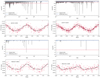 |
Fig. 5. As in Fig. 3 but for the UHE white dwarfs J1215+1203, J1257+4220, HS 2027+0651, and HS 2115−1148. |
J1257+4220. This object is a DA-type UHE white dwarf and was observed in the course of the CSS, ZTF, and ATLAS. While in the CSS V-band and ATLAS o-band no significant periodic signal can be detected, the ZTF light curves and ATLAS c-band light curves indicate the strongest periodic signal at P ≈ 0.43 d. Heinze et al. (2018) classified J1257+4220 as a sinusoidal variable with significant residual noise and, again, reports twice the period (P = 0.857925 d) found by us.
J1510+6106 is a DO UHE white dwarf and two minute cadence light curves are available from four TESS sectors. There are no blends with other stars in the TESS aperture or a contamination by nearby bright stars (Fig. 2). In the periodogram of the combined TESS light curve, we find one significant peak at 5.187747 d (log(FAP) = − 5.1), however this signal is not found in any individual sector light curve. This white dwarf was also observed more than 500 times in both the ZTF g- and r-band. No significant periodic signals can be found in those light curves. Thus, we remain skeptical about the five-day period from the combined TESS light curve, and classify this star only as a possibly variable.
HS 2027+0651. This object is a DO UHE white dwarf that was observed within the ZTF. The periodogram of the ZTF g-band light curve indicates P ≈ 0.29 d. The amplitude of the phase-folded light curve is 0.06 mag, and its minimum is again broad and flat (bottom left panel in Fig. 5).
HS 2115−1148. This object is a DAO-type UHE white dwarf with very weak UHE lines. The periodogram of the ZTF r-band (Fig. 6) predicts the strongest signal around 1.32 d. The amplitude of the phase-folded light curve is 0.04 mag.
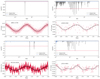 |
Fig. 6. As in Fig. 3 but for the He II line problem white dwarfs J0821+1739 and J1029+2540, HE 1314+0018, and J1512+0651. |
3.2.2. White dwarfs showing only the He II line problem
J0821+1739. This is the faintest object in our sample (G = 19.07 mag). In the periodogram (top row left in Fig. 6) of the K2 light curve processed by the EVEREST pipeline only one strong signal can be found at P = 0.384875 d. This variability is already clearly visible in the (unfolded) light curve. We note that both the amplitude and shape of the phase-folded K2 light curve must not be regarded as reliable due to the long exposure time (5% of the period). The ≈0.38 d period is also confirmed by the K2 light curve processed by the K2SFF pipeline, although we obtain a higher FAP for the variability. Even though the target is quite faint, we also find the ≈0.38 d period in the CSS and ZTF g-band light curves. However, this period is not significant (log(FAP) = − 3.0 < 4) in the latter. The amplitude of the phase-folded CSS light curve is 0.13 mag.
J0827+5858. This object was observed 332 times in the course of the CSS (V = 17.46 mag), and about 200 times in both the ZTF g- and r-bands. We do not find a significant periodic variability in any of those light curves.
J0947+1015. This source was observed 447 times in the course of the CSS (V ≈ 18.07 mag), and 64 and 81 times in the ZTF g- and r-bands, respectively. The periodogram of the CSS light curve indicates a period of 0.257938 d with an associated log(FAP) = − 3.6. The amplitude of the phase-folded light curve is 0.10 mag. We classify this star as a possibly variable.
J1029+2540. In the periodogram of the ZTF g-band light curve for this object we find the strongest periodic signal in the ZTF g-band around P = 0.28 d (first row right in Fig. 6). This period is confirmed by the CSS V-band and ZTF r-band data.
HE 1314+0018. We find a significant period around 0.52 d in the TESS data of this fairly bright (G = 16.05 mag) star. The amplitude of the phase folded light curve is only 0.03%. After the first whitening cycle no other significant peak remains in the periodogram (penultimate row left of Fig. 6). The star was also observed 368 times within the CSS, but no significant periodic signal can be found in this data set.
J1512+0651. This source has been observed 103 and 119 times in the ZTF g- and r-band, and 365 times in the CSS V-band. We find the strongest signal at 0.226 d in the periodogram of the ZTF r band. We also find the 0.226 d period in the ZTF g and CSS V band, albeit at FAPs below our threshold. The amplitude of the phase-folded ZTF r band light curve is 0.06 mag.
HS 1517+7403. In the periodograms of the ZTF g- and r-band light curves we find the strongest signals around 1.09 d, respectively. After the first whitening cycle, no other significant signal remains. The star was also observed with TESS. The periodogram of the TESS light curve predicts the strongest peak around 8.78 d, but another strong signal is detected at 1.09 d confirming what is found from the ZTF light curves. Because we do not see a significant peak at around 8.78 d in the ZTF periodograms, we adopt 1.09 d as the photometric period of the star. After whitening the TESS light curve for the 1.09 d period (including it harmonics and subharmonics), the signal at 8.78 d disappears, but other significant signals around 7 d and 2 d remain. As these latter signals are not detected in the ZTF periodograms, we conclude that they most likely originate from the other star(s) inside the aperture mask, or the two-orders-of-magnitude-brighter star right next to it (bottom row, right of Fig. 2).
J1553+4832. This faint (G = 18.65 mag) object was observed about 1200 times in the course of the ZTF. In both the periodograms of the ZTF g and r band, we find the strongest signals around 2.93 d. The amplitudes of the phase-folded light curves in both bands is about 0.05 mag. We note that there are also aliases at lower periods (e.g., at 1.52 d and 0.74 d), which have a similar FAP (all of them are removed after the first whitening cycle). Thus, it may be possible that the real photometric period is shorter. The star was also observed 171 times within the CSS, but no significant periodic signal can be found in this light curve.
4. Overall results
4.1. Variability rates
We find that 12 out of the 16 UHE white dwarfs are significantly photometrically variable, meaning their light curves exhibit periodic signals with a log(FAP) ≤ − 4. This leads to a variability rate of  %. Given the low-number statistics, the uncertainties were calculated assuming a binomial distribution and indicate the 68% confidence-level interval (see e.g., Burgasser et al. 2003). For two objects, HE 0504−2408 and HS 0742+6520, we find periodic signals with associated log(FAPs)≈ − 3. For J1510+6106 we do not trust the signal around 5.19 d discovered in the combined TESS light curve, because it can neither be found in the ZTF g or r band light curve (about 500 data points each), nor in the four individual TESS light curves. Those latter three objects we consider as possibly variable. For the DA-type UHE white dwarf J0900+2343, no hint of variability could be found, which might nevertheless be a consequence of the faintness of the star (G = 18.79 mag). For the white dwarfs that show only the He II line problem, we find a similar variability rate of
  %, meaning that six out of the eight He II line problem white dwarfs are significantly photometrically variable. For J0827+5858 we cannot find a significant periodic signal, and J0947+1015 we classify as possibly variable. The high photometric variability rate amongst these stars suggests that the UHE and He II line problem phenomena are linked to variability.
However, it is not yet clear whether the photometric variability is indeed an intrinsic characteristic of these stars alone, or is rather something that is observed amongst all very hot white dwarfs. In order to clarify this matter, we obtained ZTF DR4 light curves of a comparison sample and searched for photometric variability in those light curves as well. Our comparison sample consists of several very hot (Teff ≥ 65 000 K) DO-type (55 in total, including 28 PG 1159-type stars) white dwarfs from Dreizler & Werner (1996), Dreizler & Heber (1998), Hügelmeyer et al. (2005, 2006), Werner & Herwig (2006), Werner et al. (2014), and Reindl et al. (2014, 2018), as well as very hot (Teff ≥ 65 000 K) DA-type (90 in total) white dwarfs from the samples of Gianninas et al. (2011) and Tremblay et al. (2019). We considered only ZTF light curves that have at least 50 data points (this was found from our previous analysis to be the approximate number of points needed to detect periodic signals in the ZTF data). We find that amongst the H-deficient white dwarfs, only one of the 41 objects with sufficient data points in the ZTF is significantly variable (variability rate:  %)3. For the H-rich white dwarfs, we find a higher variability rate of
  % (59 stars had at least 50 data points and eight turned out to be significantly variable). In Table A.3, we list all of the normal white dwarfs which we found to be variable based on the ZTF data, including the mean magnitudes, derived periods, and amplitudes. The variability rate of all normal white dwarfs together is then
  %, in stark contrast to the combined variability rate of
  % based on ZTF data for the UHE and He II line problem white dwarfs4. Thus, we conclude that periodic photometric variability is indeed a characteristic of UHE and He II line problem white dwarfs.
4.2. Light-curve shapes
The shapes of the light curves are quite diverse. Some objects show near perfect sinusoidal variations (e.g., HE 1314+0018, J1029+2540), while the light curves of seven objects in our sample (about one-third amongst the variable ones) show extended, flat minima (J0254+0058, J0146+3236, HS 0713+3958, HS 0727+6003, HS 2027+0651, J1553+4832, and HS 1517+7403). Particularly interesting are the light curves of HS 0158+2335, that show two uneven maxima. This might also be the case for J1512+0651 (shows only the He II line problem), though higher S/N light curves would be needed to confirm this.
4.3. Amplitudes
The amplitudes of the light-curve variations range from a few hundredths of a magnitude to a few tenths of a magnitude. For a given object, the amplitudes in the different bands do not vary significantly. This means that we find that the difference in the amplitudes as measured in the different bands is smaller than or equal to the standard deviation of the difference between the observations and our mathematical fit (black lines in Figs. 3–7). In particular, the SDSS stripe 82 light curves of J0254+0058 (the only object in our sample with u to z band data) do not indicate an increase in the amplitudes towards shorter or longer wavelengths. Also, in the BUSCA light curves of HS 0727+6003 (only other object with U-band light curve) we found no hint of a difference in the amplitudes.
We note that we do not trust the amplitudes of the TESS light curves. This is because the TESS mission was designed for stars brighter than 15 mag, and all our targets are fainter than this. Further, the large pixel size implies that an accurate background subtraction is very complicated, in particular in crowded fields. The majority of the TESS light curves predict amplitudes that are larger than what is observed in the other bands. For example, the amplitude of the phase-folded TESS light curve of J0254+0058 is 0.54 mag, which almost twice that observed in the other bands (≈0.3 mag). If this large TESS amplitude were real, we would expect to see similarly large amplitudes in the SDSS i- and z-band as well, but this is not the case. The faintness of our targets and the large TESS pixel size of 21 arcsec – which often leads to contamination from neighboring stars – also result in a large scatter in the TESS light curves. This in combination with the shorter duration of the TESS light curves compared to those obtained from ground-based surveys like ZTF (about one month compared to more than two years) explains the larger uncertainties on the periods obtained from the TESS data.
4.4. Periods
The photometric periods of the UHE white dwarfs range from 0.22 to 2.32 d, with a median of 0.69 d and a standard deviation of 0.59 d. For the six photometrically variable white dwarfs showing only the He II line problem, we find a very similar period range from 0.22 to 2.93 d, with a median of 0.45 d and a standard deviation of 0.95 d. Considering both classes together we find a median of 0.56 d with a standard deviation of 0.73 d.
The observed periods are consistent with typical white dwarf rotational rates (Kawaler 2004; Hermes et al. 2017a), but could also indicate post-common envelope (PCE) binaries (Nebot Gómez-Morán et al. 2011). It is therefore worth comparing the period distribution of those objects to the period distribution of our sample in detail.
Figure 8 shows the combined period distribution of the UHE white dwarfs and white dwarfs showing only the He II line problem. The left panel shows a comparison of their period distribution to the orbital period distribution of confirmed post-common envelope (PCE) binary central stars of planetary nebulae (CSPNe; light green, Jones & Boffin 2017; Boffin & Jones 2019)5 and PCE white dwarf and main sequence binaries (light yellow) from the sample of Nebot Gómez-Morán et al. (2011). The right panel shows a comparison with the rotational periods of pulsating white dwarfs (light green with dashed contours; values taken from Kawaler 2004; Hermes et al. 2017a) and apparently single magnetic white dwarfs (bold yellow lines, values taken from Ferrario et al. 2015). We note that there are also a few longer period magnetic white dwarfs (Putney & Jordan 1995; Bergeron et al. 1997; Schmidt et al. 1999; Kawka & Vennes 2012) and PCE binary central stars (Miszalski et al. 2018a,b; Brown et al. 2019) that we omit from Fig. 8 for better visualization. From this figure it already seems that the period distribution of our sample more closely resembles the period distribution of PCE binaries than the rotational period distribution of white dwarfs. The median rotational period of nonmagnetic white dwarfs is 1.20 d, while the median period of our sample is half of that. The observed rotational periods of magnetic white dwarfs as determined from polarimetry and photometry range from a few minutes, through hours and days, to over decades and centuries. The short-spin-period white dwarfs show their peak near 0.1 d, a period much shorter than what we observe for the UHE white dwarfs and white dwarfs showing the He II line problem.
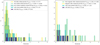 |
Fig. 8. Distribution of the photometric periods of the variable UHE and He II line problem white dwarfs (blue), and the period distribution of only the UHE white dwarfs (purple). On the left their period distribution is compared to the orbital period distribution of PCE CSPNe (light green; the bold teal line indicates the period distribution of binary CSPNe that show a reflection effect) and white dwarfs plus main sequence binaries (light yellow). Left panel: a comparison with the rotational periods of normal white dwarfs (light green with dashed contours) and magnetic white dwarfs (bold yellow lines). The median period and standard deviation of each sample is indicated. |
In order to test the statistical significance of this impression we performed two-sample Kolmogorov–Smirnov tests. This test allows us to compare two samples and to check the equality of their one-dimensional probability distributions without making specific distributional assumptions. The statistical analysis is based on a D-value that represents the maximum distance between the empirical cumulative distribution function of the sample and the cumulative distribution function of the reference distribution. Based on the D-value, we then calculate the p-value, which is used to evaluate whether or not the outcomes differ significantly; this latter is a measure of the probability of obtaining test results at least as extreme as the results actually observed, assuming that the null hypothesis is correct. In our case, the null hypothesis is that the two samples compared follow the same distribution. A p-value of one indicates perfect agreement with the null hypothesis, while a p-value approaching zero rejects the null hypothesis. We performed these tests for the various samples mentioned above. First, we find that the period distributions of both UHE white dwarfs, and white dwarfs showing only the He II line problem agree with each other (p = 1.00). We also find that the period distribution of our sample agrees with that of PCE white dwarfs plus main sequence binaries (p = 0.42) and PCE CSPNe (p = 0.60 for all binary CSPNe and p = 0.25 for only the binary CSPNe showing a reflection effect). No agreement is found with the rotational period distribution of magnetic (p = 0.007), and nonmagnetic white dwarfs (p = 0.04).
However, we should keep in mind that the stars in our sample are in earlier evolutionary stages compared to the white dwarfs with measured rotational periods. According to Althaus et al. (2009), the radius of a DO white dwarf with typical mass of 0.6 M⊙ decreases from 0.017 R⊙ to 0.013 R⊙ while the star cools down from 80 000 K (typical Teff for a UHE white dwarf) to 20 000 K (the majority of magnetic white dwarfs from Ferrario et al. 2015 are reported to have temperatures below this value, as are all of the nonmagnetic white dwarfs from Kawaler 2004; Hermes et al. 2017a). If we assume conservation of angular momentum then the rotational period should decrease approximately by a factor of 0.5. Therefore, we repeated the statistical tests under the simplified assumption that all of the objects in our sample will halve their periods as they cool down. We find that there is no agreement with the rotational period distribution of nonmagnetic white dwarfs (p = 0.0001), but that there is a statistically meaningful agreement with the rotational period distribution of magnetic white dwarfs (p = 0.11).
5. Discussion
We find that both UHE and He II line problem white dwarfs overlap in a narrow region in the Gaia HRD. As expected, they lie on top of the white dwarf banana and are well separated from the hot subdwarf stars, and are much bluer than similarly hot white dwarfs with M dwarf companions. On average, UHE white dwarfs are found to be slightly bluer and have slightly brighter absolute G-band magnitudes than the white dwarfs showing only the He II line problem. This might suggest that white dwarfs with UHE lines could evolve into objects that show only the He II line problem. However, better constraints on the temperatures of these stars as well as a larger sample would be needed to investigate this possibility further.
Our light curve studies reveal that the majority of both the UHE white dwarfs ( %) and He II line problem white dwarfs (
 %) are photometrically variable. The fact that their photometric period distributions agree with each other, and that their light curves exhibit similar amplitudes and shapes, reinforces the hypothesis that both classes are indeed related. What remains to be discussed is the cause of the photometric variability and how it is linked to the occurrence of the UHE features and He II line problem.
The photometric periods of all stars in our sample are well above the theoretical upper limit of 104 s predicted for nonradial g-mode pulsations that are frequently observed amongst PG 1159 stars (most of them having periods below 3000 s; Quirion et al. 2007; Córsico et al. 2019, 2021). Thus, we see two possible scenarios that could instead account for the photometric variability in our stars; one is linked to close binaries, and the other one related to magnetic fields.
5.1. Binaries
Because of the very good agreement of the period distribution of our stars with that of PCE systems, an obvious assumption is that our stars are close binaries. If so, a variety of physical processes could lead to the observed periodic variability. We rule out that the objects in our sample are (over-)contact binaries, because the light curves of such systems have extended maxima and narrow (sometimes V-shaped) photometric minima and also often two uneven minima (e.g., Miszalski et al. 2009; Drake et al. 2014). Also, ellipsoidal deformation, which occurs in a detached system where one star is distorted due to the gravity of its companion, can be ruled out as the main source for the photometric variability. This is because the amplitudes of the light-curve variations caused by ellipsoidal deformation in systems that contain a hot and compact white dwarf and an extended companion are always much smaller than that from the so-called irradiation effect.
An irradiation or reflection effect caused by the heated face (day-side) of a cooler companion whose rotational period is synchronized to the orbital period appears to be a likely scenario. Irradiation binaries display sinusoidal light-curve variations, but when the system is seen under a high inclination angle, the light curves have extended and flat photometric minima, which is precisely what we find for seven objects in our sample (Sect. 4.2). Well-studied examples that exhibit this latter kind of light curve are the hot subdwarf plus M-dwarf binary HS 2333+3927 (Heber et al. 2004), and the hot white dwarf plus M-dwarf binaries HS 1857+5144 (Aungwerojwit et al. 2007) and NN Ser (which also shows eclipses, Brinkworth et al. 2006). The observed amplitudes can be as low as 0.01 mag and reach up to about 1 mag (Shimansky et al. 2006; Brinkworth et al. 2006), covering the observed amplitude range of our objects. However, we see serious problems with the irradiation effect system scenario. First, we would expect to find – at least for some objects – noticeable differences in the amplitudes observed in the different bands. For example, in the very hot (Teff ≥ 49 500 K) white dwarf plus low-mass main sequence star irradiation systems SDSS J212531.92−010745.9, and the central stars of Abell 63, V477 Lyr, ESO330–9, and PN HaTr 7, the ratio of the R-band to V-band amplitude ranges from 1.13 to 1.38 (Shimansky et al. 2015; Afşar & Ibanoǧlu 2008; Hillwig et al. 2017). WD1136+667 and NN Ser even display r-band to g-band amplitude ratios of 1.44 and 1.67, respectively (shown by the present study, and Brinkworth et al. 2006). An even larger difference in the amplitudes – by a factor of almost two – is expected when u-band photometry is also available (De Marco et al. 2008). This should be easily noticeable in the light curves of J0254+0058 and HS 0727+6003.
In order to test this we calculated reflection-effect models for the SDSS-ugriz light curves of J0254+0058. We used the code LCURVE (for details, see Appendix A of Copperwheat et al. 2010), which was developed for white dwarfs plus M-dwarf systems and has been used to fit detached or accreting white dwarfs plus M-dwarf and hot subdwarf plus M-dwarf systems showing a significant reflection effect (see Parsons et al. 2010; Schaffenroth et al. 2021, for more details). For that we assumed Teff = 80 000 K for the white dwarf (Hügelmeyer et al. 2006) and typical values for the masses and radii of white dwarfs plus M-dwarf systems (q = 0.21, R1 = 0.02 R⊙, R2 = 0.15 R⊙, Parsons et al. 2010). To find a first good model we fitted the SDSS-r light curve by letting the inclination i, the temperature of the companion T2, and the albedo of the companion vary. We found a perfectly fitting model for an inclination of i = 86.8° and a temperature of the companion of T2 = 4500 K. To see if this is also consistent in the other bands, we fixed the stellar parameters of both stars and derived light curve models for the other bands. We were only able to fit the light curve if the albedo of the companion was varied significantly (A = 0.6 in SDSS-z to A = 3.5 in SDSS-u, dashed line in Fig. 9). Such a large change in the albedo is unphysical, as the albedo gives the percentage of the flux from the white dwarf that is used to heat up the irradiated side of the companion. If we assume an albedo of A = 1, the amplitude of the light curve varies significantly from smaller in the blue to larger in the red, as shown in Fig. 9.
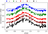 |
Fig. 9. SDSS-ugriz light curves of J0254+0058. The solid line shows the light curve models using the parameters derived by fitting the SDSS-r light curve and a fixed albedo of A = 1 in all bands. The dashed lines give the light curve model fit that allows for unphysical variations in the albedo of the companion. |
As explained before, this increase in the amplitude of the reflection effect from blue to red is expected. The amplitude of the reflection effect is calculated as the difference in the flux between phase 0, where the white dwarf and the maximum projected area of the cool side of the companion is visible, and phase 0.5, where the white dwarf and the maximum projected area of the heated side of the companion is visible. Depending on the temperature of the white dwarf and the orbital separation of the system, the companion is heated up to around 10 000 − 20 000 K. As the white dwarf has maximum flux in the UV, the contribution of the companion increases from blue to red.
To simulate this, we used the parameters that we derived in the light curve fit and used a black body approximation to calculate the amplitude of the reflection effect as a function of the temperature of the heated side of the companion. As the period of the putative binary system is relatively long, we calculated amplitudes up to 8000 K for the heated side of the companion. This is shown in Fig. 10. A significant increase in the amplitude from SDSS-u (5%) to SDSS-z (40%) is predicted, which is not observed. From Fig. 10 it also becomes clear that the amplitude in the r band should be about twice that in the g band. However, none of the ten other objects, which show significant periodic variations in both ZTF bands, show an increased amplitude in the r band compared to the g band.
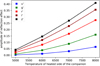 |
Fig. 10. Expected amplitude for J0254+0058 of the reflection effect as a function of the temperature of the heated side of the companion. The amplitude was calculated as the difference in flux of a white dwarf and a M-dwarf companion with the parameters derived in the light curve fit in phase 0 and phase 0.5 using a black-body approximation. |
The second drawback of the reflection effect scenario is that none of our stars exhibit spectral features of a cool secondary (Figs. B.1 and B.2). As mentioned before, a late-type M dwarf or a brown dwarf may easily be outshined by the still luminous white dwarf, and therefore the nondetection of an increased continuum flux in the optical or lack of (molecular) absorption features from the companion cannot be taken as irrefutable evidence. However, to the very best of our knowledge, without exception all PCE systems containing a very hot (Teff ≥ 60 000 K) white dwarf primary (and even those who outshine their cool companions in the optical) exhibit emission lines (e.g., the Balmer series or the CNO complex around 4650 Å) arising from the highly irradiated hemisphere of a secondary. These emission lines are typically quite strong and can therefore also be detected in low-resolution (e.g., SDSS) spectra (Nagel et al. 2006; Nebot Gómez-Morán et al. 2011). It is also well known that the emission lines appear and disappear over the orbital cycle, reaching maximum strength at photometric maximum. Thus, it may be possible that the emission lines are not detectable when the systems are observed close to the photometric minimum. However, it is very unlikely that all spectra of the stars in our sample were taken at that same phase.
For a reflection effect, the amplitudes of the light-curve variations are expected to be correlated with the temperature of the day-side of the irradiated companion. If we assume that all hypothetical close companions to our stars have the same temperature, then the amplitudes should correlate with L/P2/3, where L is the luminosity of the white dwarf and P the orbital (photometric) period. This means that more luminous primaries at shorter orbital periods are expected to cause a larger reflection effect than less luminous primaries at longer periods. However, using MG0 as a proxy for L, no correlation between MG0/P2/3 and the mean amplitudes is found (Pearson correlation coefficient: r = −0.01)67. This serves as a third argument against our stars being reflection-effect binaries.
Finally, we would like to note that, if the variability in all our objects were found to indeed be caused by close companions, this would imply an exceptionally high compact binary fraction amongst H-deficient stars of 30%8. Of the immediate precursors of DO-type white dwarfs, only one O(He) star and one luminous PG 1159 star9 are known to be radial-velocity variable (Reindl et al. 2016). Another O(He)-type star, the central star of Pa 5, shows photometric variability of 1.12 d, which nevertheless might also be attributed to spots on its surface (De Marco et al. 2015). Although no systematic search for close binaries has yet been conducted for PG 1159 and O(He) stars, this would lead us to an estimated close binary fraction in the H-deficient pre-white dwarfs of 11.5%, which is a factor of 2.6 below what would be needed to explain the variability in our stars via close binaries.
5.2. Magnetic fields
The fraction of the hottest white dwarfs that show UHE lines or the He II line problem (about 10%) matches the fraction of magnetic white dwarfs (2−20% are reported, Liebert et al. 2003; Giammichele et al. 2012; Sion et al. 2014; Kepler et al. 2013, 2015). In addition, we find that the period distribution of our stars agrees with that of magnetic white dwarfs if we assume that they will spin up as a consequence of further contraction. Proposing that UHE white dwarfs are magnetic, Reindl et al. (2019) suggested that optically bright spots on the magnetic poles and/or geometrical effects of a circumstellar magnetosphere could be responsible for the photometric variability in J0146+3236.
Spots on hot white dwarfs are expected to be caused by the accumulation of metals around the magnetic poles (Hermes et al. 2017b). This is also the case for chemically peculiar stars, where the magnetic field produces large-scale chemical abundance inhomogeneities causing periodic modulations of spectral line profiles and light curves (Oksala et al. 2015; Prvák et al. 2015, 2020; Krtička et al. 2018, 2020a; Momany et al. 2020). This is understood as a result from the interaction of the magnetic field with photospheric atoms diffusing under the competitive effects of gravity and radiative levitation (Alecian & Stift 2017). If the radiative and gravitational forces are of similar orders of magnitude, these structures are able to form and subsist (Wade & Neiner 2018). In fact, it was found by Reindl et al. (2014) that the DO-type UHE and He II line problem white dwarfs are located at this very region in the Teff − log g diagram, where also the wind limit as predicted by Unglaub & Bues (2000) occurs. This further supports the hypothesis that effects of gravitational settling and radiation-driven mass loss are about the same in our stars, and that long-lived spots can therefore be expected.
Reindl et al. (2019) showed that the light curve of J0146+3236 can be modeled assuming two uneven spots whose brightness is slightly over 125% relative to the rest of the stellar surface. In order to get an idea of the metal enhancement needed to achieve such an increase in brightness, we calculated test models with TMAP. In the model atmosphere calculations, we assumed Teff = 80 000 K, log g = 8.0, and included opacities of He and the iron-group elements (Ca, Sc, Ti, V, Cr, Mn, Fe, Co, and Ni), of which Fe was found to be the most abundant trace element in UHE white dwarfs (Werner et al. 2018b). Iron-group elements were combined in a generic model atom, using a statistical approach, employing seven superlevels per ion linked by superlines, together with an opacity-sampling method (Anderson 1989; Rauch & Deetjen 2003). Ionization stages IV−VII augmented by a single ground-level stage VIII were considered and we assumed solar abundance ratios. The models were calculated for metallicities of 10−3, 10−2, and 10−1 (mass fractions). In addition, we calculated a model including, in addition to He, opacities of C, and O at typical abundance values of low-luminosity PG 1159 stars (mass fractions of 5 × 10⁻², and 1 × 10⁻², respectively). For the calculations, we considered ionization stages III−V and III−VII for C and O, respectively, and a total of 404 NLTE levels. Finally, a pure He model was also computed. After that, the model fluxes were convolved with filter response functions of the Galex FUV, NUV, and the SDSS u, g, r, i, and z bands in order to calculate synthetic magnitudes.
Figure 11 shows the various synthetic spectra, and the filter response functions are indicated. The differences in the resulting magnitudes relative to our pure He model are listed in Table 2. We find that with an increasing abundance of the iron-group elements, the continuum flux becomes steeper towards the UV. Most of the bound-bound transitions are located at FUV wavelengths at this effective temperature, which in turn causes a flattening of total flux in the FUV band (upper panel in Fig. 11). Comparing our pure He model to our model that also contains C and O, we find that the continuum flux also increases from the near-infrared (NIR) to the far-UV, and therefore also produces optically bright spots. However, because many strong bound-bound transitions of C and O are located in the optical (especially in the SDSS g band; lower panel in Fig. 11), the behavior of the amplitude differences varies significantly from our models with iron-group elements. This has been shown for a Cen by Krtička et al. (2020b), where for example an enhancement in He, Si, or Fe not only predicts a different amplitude, respectively, but also the maxima of the light curve variations are found to occur at different phases.
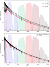 |
Fig. 11. Differences in the flux of models with different metal contents and a model containing only He (red). Upper panel: fluxes for different abundances of the iron-group elements, and lower panel: a model that contains opacities of He, C, and O. The filter response functions of the Galex FUV, NUV, and SDSS u, g, r, i, and z bands are indicated. |
Predicted differences in the resulting magnitudes from synthetic spectra containing metals relative to a model containing only He.
We also note that because spots cover only a part of the stellar surface, the amplitudes listed in Table 2 can be seen merely as an upper limit of what could be expected observationally from the metal enhancement in the spot. Nevertheless, this demonstrates that chemical spots could indeed explain the relatively large amplitude variations we see in our stars. The only drawback is that, for all the metals considered here, the predicted amplitude in the u band is always significantly larger than in the redder bands. This is not observed for the two stars in our sample for which we have u band light curves. However, only time-resolved UV spectroscopy combined with detailed light curve modeling will be able to shed light on which enhancement of elements is responsible for the observed light curve variability and whether or not chemical spots are indeed the source of the variability.
Besides a chemically inhomogeneous photosphere, stellar magnetism can create another source of photometric variability. Munoz et al. (2020) recently hypothesized that the photometric variability observed in magnetic O-type stars is a consequence of electron scattering in the obliquely rotating magnetosphere, which periodically occults the stellar disk. These latter authors presented theoretical light curves for various inclinations, i, and magnetic obliquity angles, β, mass-feeding rates, magnetic field strengths, terminal wind velocities, and smoothing lengths. Increasing the latter four parameters, they find that the amplitude of the light-curve variations should increase. For low inclination and obliquity angles, they find roughly sinusoidal light-curve variations. When i + β > 90°, the magnetic equator crosses the observer’s line-of-sight twice per rotation cycle and a second maximum in the light curve shows up. Interestingly, for intermediate inclination and obliquity angles (e.g., i = β = 50°), their models predict a relatively long, and almost flat photometric minimum, which is precisely what we observe for seven of our stars. One of these stars is J0146+3236 for which Reindl et al. (2019) already suggested i ≈ β ≈ 45°. Also, the models of Munoz et al. (2020) predict that the photometric minimum should occur when the circumstellar magnetosphere is seen edge-on, that is, when the column density of the magnetospheric material occulting the stellar disk is highest. The magnetospheric occultation model might even be able to explain the extraordinary light curve of HS 0158+2335, which exhibits two uneven maxima. Its light curve resembles that of LMCe136–1, which could be reproduced by Munoz et al. (2020) assuming a dipolar offset model.
6. Conclusions
Our work reveals exceptionally high photometric variability rates amongst both UHE white dwarfs and white dwarfs that show only the He II line problem, marking them a new class of variable stars. We find further evidence that both classes are indeed related, as concluded from their overlap in the Gaia HRD, similar photometric variability rates, light curve shapes and amplitudes, and period distributions. While an irradiation effect could explain their observed period distribution, and the shapes of their light curves, we believe that this scenario is unlikely. This is because we do not detect increasing amplitudes towards longer wavelengths in any object, nor do we see emission lines arising from the strongly irradiated side of a hypothetical close binary. Instead, we hold on to the suggestion of Reindl et al. (2019) that the variability is caused by magnetic spots and/or the co-rotating, circumstellar material.
Further investigations are needed for a profound understanding of these special objects. A systematic search for radial-velocity variations, as well as an IR excess in combination with detailed light-curve modeling, will help to clarify whether or not the close binary scenario can really be ruled out. On the other hand, the spots/magnetosphere scenario can be verified with spectro-polarimetric observations and time-resolved UV (where photospheric metals can be detected) spectroscopy, which in turn could reveal the magnetic field strengths and chemical spots, respectively. Last but not least, the discovery that the majority of the UHE and He II line problem white dwarfs are photometrically variable provides an important observational constraint that can be used to detect more of these systems.
The term “white dwarf banana” was coined by Girven et al. (2011).
We note that the ZTF data are not suitable to detect pulsations. Otherwise a higher variability rate could be expected for very hot H-deficient white dwarfs, as many of them are GW Vir pulsators.
Amongst the UHE and He II line problem white dwarfs 21 objects have at least 50 data points in at least one ZTF band, and 14 of them turned out to be variable based on the ZTF data.
We only used objects with a relative uncertainty for the parallax smaller than 20% to check for this correlation.
The inclination angle of the system also has an impact on the amplitudes, which would cause an additional scatter. However, it is unlikely that the inclinations are distributed in such a way that the correlation between the amplitude and MG0/P2/3 simply vanishes.
30% of all DO-type white dwarfs hotter than 65 000 K show UHE lines or only the He II line problem. If we exclude those that are classified as PG 1159 stars (C/He > 0.02, number fraction) from the group of normal DO-type white dwarfs, we obtain a value of 47%.
Only ten O(He) stars and 16 PG 1159 pre-white dwarfs (log g < 7.0) are known.
Acknowledgments
We thank Jiri Krtička, Thomas Kupfer, and JJ Hermes for helpful comments. We thank Stefan Dreizler for providing us with the TWIN spectrum of HS1517+7403. VS is supported by the Deutsche Forschungsgemeinschaft, DFG through grant GE 2506/9-1. IP acknowledges support from the UK’s Science and Technology Facilities Council (STFC), grant ST/T000406/1. IP was partially supported by the Deutsche Forschungsgemeinschaft, DFG through grant GE2506/12-1. The BUSCA observing run was made possible with support from STFC grant ST/T001380/1. Some of the data presented in this paper were obtained from the Mikulski Archive for Space Telescopes (MAST). This research has made use of NASA’s Astrophysics Data System and the SIMBAD database, operated at CDS, Strasbourg, France. Based on observations collected at the German-Spanish Astronomical Center, Calar Alto, jointly operated by the Max-Planck-Institut für Astronomie Heidelberg and the Instituto de Astrofísica de Andalucía (CSIC). Based on data obtained from the ESO Science Archive Facility under request number nreindl/584030. The TMAD (http://astro.uni-tuebingen.de/~TMAD) and TIRO tool (http://astro.uni-tuebingen.de/~TIRO) used for this paper was constructed as part of the activities of the German Astrophysical Virtual Observatory. This work has made use of data from the European Space Agency (ESA) mission Gaia (https://www.cosmos.esa.int/gaia), processed by the Gaia Data Processing and Analysis Consortium (DPAC, https://www.cosmos.esa.int/web/gaia/dpac/consortium). Funding for the DPAC has been provided by national institutions, in particular the institutions participating in the Gaia Multilateral Agreement. The CSS survey is funded by the National Aeronautics and Space Administration under Grant No. NNG05GF22G issued through the Science Mission Directorate Near-Earth Objects Observations Program. The CRTS survey is supported by the U.S. National Science Foundation under grants AST-0909182 and AST-1313422. Based on observations obtained with the Samuel Oschin 48-inch Telescope at the Palomar Observatory as part of the Zwicky Transient Facility project. ZTF is supported by the National Science Foundation under Grant No. AST-1440341 and a collaboration including Caltech, IPAC, the Weizmann Institute for Science, the Oskar Klein Center at Stockholm University, the University of Maryland, the University of Washington, Deutsches Elektronen-Synchrotron and Humboldt University, Los Alamos National Laboratories, the TANGO Consortium of Taiwan, the University of Wisconsin at Milwaukee, and Lawrence Berkeley National Laboratories. Operations are conducted by COO, IPAC, and UW. This work includes data from the Asteroid Terrestrial-impact Last Alert System (ATLAS) project. ATLAS is primarily funded to search for near earth asteroids through NASA grants NN12AR55G, 80NSSC18K0284, and 80NSSC18K1575; byproducts of the NEO search include images and catalogs from the survey area. The ATLAS science products have been made possible through the contributions of the University of Hawaii Institute for Astronomy, the Queen’s University Belfast, the Space Telescope Science Institute, and the South African Astronomical Observatory. This paper includes data collected by the TESS mission. Funding for the TESS mission is provided by the NASA Explorer Program. This work made use of tpfplotter by J. Lillo-Box (publicly available in www.github.com/jlillo/tpfplotter), which also made use of the python packages astropy, lightkurve, matplotlib, and numpy. IRAF is distributed by the National Optical Astronomy Observatory, which is operated by the Association of Universities for Research in Astronomy (AURA) under a cooperative agreement with the National Science Foundation. Funding for the Sloan Digital Sky Survey IV has been provided by the Alfred P. Sloan Foundation, the US Department of Energy Office of Science, and the Participating Institutions. SDSS-IV acknowledges support and resources from the Center for High Performance Computing at the University of Utah. The SDSS website is www.sdss.org. SDSS-IV is managed by the Astrophysical Research Consortium for the Participating Institutions of the SDSS Collaboration including the Brazilian Participation Group, the Carnegie Institution for Science, Carnegie Mellon University, Center for Astrophysics, Harvard & Smithsonian, the Chilean Participation Group, the French Participation Group, Instituto de Astrofísica de Canarias, The Johns Hopkins University, Kavli Institute for the Physics and Mathematics of the Universe (IPMU)/University of Tokyo, the Korean Participation Group, Lawrence Berkeley National Laboratory, Leibniz Institut für Astrophysik Potsdam (AIP), Max-Planck-Institut für Astronomie (MPIA Heidelberg), Max-Planck-Institut für Astrophysik (MPA Garching), Max-Planck-Institut für Extraterrestrische Physik (MPE), National Astronomical Observatories of China, New Mexico State University, New York University, University of Notre Dame, Observatário Nacional/MCTI, The Ohio State University, Pennsylvania State University, Shanghai Astronomical Observatory, United Kingdom Participation Group, Universidad Nacional Autónoma de México, University of Arizona, University of Colorado Boulder, University of Oxford, University of Portsmouth, University of Utah, University of Virginia, University of Washington, University of Wisconsin, Vanderbilt University, and Yale University.
References
- Abazajian, K. N., Adelman-McCarthy, J. K., Agüeros, M. A., et al. 2009, ApJS, 182, 543 [Google Scholar]
- Afşar, M., & Ibanoǧlu, C. 2008, MNRAS, 391, 802 [NASA ADS] [CrossRef] [Google Scholar]
- Alecian, G., & Stift, M. J. 2017, MNRAS, 468, 1023 [NASA ADS] [CrossRef] [Google Scholar]
- Aller, A., Lillo-Box, J., Jones, D., Miranda, L. F., & Barceló Forteza, S. 2020, A&A, 635, A128 [CrossRef] [EDP Sciences] [Google Scholar]
- Althaus, L. G., Panei, J. A., Miller Bertolami, M. M., et al. 2009, ApJ, 704, 1605 [NASA ADS] [CrossRef] [Google Scholar]
- Anderson, L. S. 1989, ApJ, 339, 558 [NASA ADS] [CrossRef] [Google Scholar]
- Aungwerojwit, A., Gänsicke, B. T., Rodríguez-Gil, P., et al. 2007, A&A, 469, 297 [NASA ADS] [CrossRef] [EDP Sciences] [Google Scholar]
- Bainbridge, M., Barstow, M., Reindl, N., et al. 2017, Universe, 3, 32 [Google Scholar]
- Becker, A. C., Bochanski, J. J., Hawley, S. L., et al. 2011, ApJ, 731, 17 [CrossRef] [Google Scholar]
- Bellm, E. C., Kulkarni, S. R., Graham, M. J., et al. 2019, PASP, 131 [Google Scholar]
- Berengut, J. C., Flambaum, V. V., Ong, A., et al. 2013, Phys. Rev. Lett., 111 [CrossRef] [Google Scholar]
- Bergeron, P., Ruiz, M. T., & Leggett, S. K. 1997, ApJS, 108, 339 [NASA ADS] [CrossRef] [Google Scholar]
- Boffin, H. M. J., & Jones, D. 2019, The Importance of Binaries in the Formation and Evolution of Planetary Nebulae (Berlin, New York: Springer-Verlag) [CrossRef] [Google Scholar]
- Brinkworth, C. S., Marsh, T. R., Dhillon, V. S., & Knigge, C. 2006, MNRAS, 365, 287 [NASA ADS] [CrossRef] [Google Scholar]
- Brown, A. J., Jones, D., Boffin, H. M. J., & Van Winckel, H. 2019, MNRAS, 482, 4951 [CrossRef] [Google Scholar]
- Burgasser, A. J., Kirkpatrick, J. D., Reid, I. N., et al. 2003, ApJ, 586, 512 [NASA ADS] [CrossRef] [Google Scholar]
- Chayer, P., Vennes, S., Dupuis, J., & Kruk, J. W. 2005, ApJ, 630, L169 [NASA ADS] [CrossRef] [Google Scholar]
- Copperwheat, C. M., Marsh, T. R., Dhillon, V. S., et al. 2010, MNRAS, 402, 1824 [NASA ADS] [CrossRef] [Google Scholar]
- Córsico, A. H., Althaus, L. G., Miller Bertolami, M. M., & Kepler, S. O. 2019, A&ARv, 27, 7 [NASA ADS] [CrossRef] [Google Scholar]
- Córsico, A. H., Uzundag, M., Kepler, S. O., et al. 2021, A&A, 645, A117 [EDP Sciences] [Google Scholar]
- De Marco, O., Hillwig, T. C., & Smith, A. J. 2008, AJ, 136, 323 [NASA ADS] [CrossRef] [Google Scholar]
- De Marco, O., Long, J., Jacoby, G. H., et al. 2015, MNRAS, 448, 3587 [NASA ADS] [CrossRef] [Google Scholar]
- Drake, A. J., Djorgovski, S. G., Mahabal, A., et al. 2009, ApJ, 696, 870 [Google Scholar]
- Drake, A. J., Graham, M. J., Djorgovski, S. G., et al. 2014, ApJS, 213, 9 [NASA ADS] [CrossRef] [Google Scholar]
- Dreizler, S., & Heber, U. 1998, A&A, 334, 618 [NASA ADS] [Google Scholar]
- Dreizler, S., & Werner, K. 1996, A&A, 314, 217 [NASA ADS] [Google Scholar]
- Dreizler, S., Heber, U., Napiwotzki, R., & Hagen, H. J. 1995, A&A, 303, L53 [NASA ADS] [Google Scholar]
- Eastman, J., Siverd, R., & Gaudi, B. S. 2010, PASP, 122, 935 [NASA ADS] [CrossRef] [Google Scholar]
- Ferrario, L., de Martino, D., & Gänsicke, B. T. 2015, Space Sci. Rev., 191, 111 [NASA ADS] [CrossRef] [Google Scholar]
- Gaia Collaboration (Prusti, T., et al.) 2016, A&A, 595, A1 [NASA ADS] [CrossRef] [EDP Sciences] [Google Scholar]
- Gaia Collaboration (Babusiaux, C., et al.) 2018, A&A, 616, A10 [NASA ADS] [CrossRef] [EDP Sciences] [Google Scholar]
- Gänsicke, B. T., Schreiber, M. R., Toloza, O., et al. 2019, Nature, 576, 61 [NASA ADS] [CrossRef] [Google Scholar]
- Geier, S. 2020, A&A, 635, A193 [CrossRef] [EDP Sciences] [Google Scholar]
- Geier, S., Raddi, R., Gentile Fusillo, N. P., & Marsh, T. R. 2019, A&A, 621, A38 [NASA ADS] [CrossRef] [EDP Sciences] [Google Scholar]
- Gentile Fusillo, N. P., Tremblay, P.-E., Gänsicke, B. T., et al. 2019, MNRAS, 482, 4570 [NASA ADS] [CrossRef] [Google Scholar]
- Giammichele, N., Bergeron, P., & Dufour, P. 2012, ApJS, 199, 29 [NASA ADS] [CrossRef] [Google Scholar]
- Gianninas, A., Bergeron, P., & Ruiz, M. T. 2011, ApJ, 743, 138 [NASA ADS] [CrossRef] [Google Scholar]
- Gianninas, A., Curd, B., Thorstensen, J. R., et al. 2015, MNRAS, 449, 3966 [NASA ADS] [CrossRef] [Google Scholar]
- Girven, J., Gänsicke, B. T., Steeghs, D., & Koester, D. 2011, MNRAS, 417, 1210 [NASA ADS] [CrossRef] [Google Scholar]
- Hagen, H.-J., Groote, D., Engels, D., & Reimers, D. 1995, A&AS, 111, 195 [NASA ADS] [Google Scholar]
- Hartman, J. D., & Bakos, G. Á. 2016, Astron. Comput., 17, 1 [NASA ADS] [CrossRef] [Google Scholar]
- Heber, U., Drechsel, H., Østensen, R., et al. 2004, A&A, 420, 251 [NASA ADS] [CrossRef] [EDP Sciences] [Google Scholar]
- Heinze, A. N., Tonry, J. L., Denneau, L., et al. 2018, AJ, 156, 241 [Google Scholar]
- Hermes, J. J., Gänsicke, B. T., Kawaler, S. D., et al. 2017a, ApJS, 232, 23 [Google Scholar]
- Hermes, J. J., Kawaler, S. D., Bischoff-Kim, A., et al. 2017b, ApJ, 835, 277 [NASA ADS] [CrossRef] [Google Scholar]
- Hillwig, T. C., Frew, D. J., Reindl, N., et al. 2017, AJ, 153, 24 [NASA ADS] [CrossRef] [Google Scholar]
- Howell, S. B., Sobeck, C., Haas, M., et al. 2014, PASP, 126, 398 [NASA ADS] [CrossRef] [Google Scholar]
- Hoyer, D., Rauch, T., Werner, K., Kruk, J. W., & Quinet, P. 2017, A&A, 598, A135 [NASA ADS] [CrossRef] [EDP Sciences] [Google Scholar]
- Hoyer, D., Rauch, T., Werner, K., & Kruk, J. W. 2018, A&A, 612, A62 [NASA ADS] [CrossRef] [EDP Sciences] [Google Scholar]
- Hu, J., Webb, J. K., Ayres, T. R., et al. 2021, MNRAS, 500, 1466 [Google Scholar]
- Hügelmeyer, S. D., Dreizler, S., Werner, K., et al. 2005, A&A, 442, 309 [NASA ADS] [CrossRef] [EDP Sciences] [Google Scholar]
- Hügelmeyer, S. D., Dreizler, S., Homeier, D., et al. 2006, A&A, 454, 617 [NASA ADS] [CrossRef] [EDP Sciences] [Google Scholar]
- Isern, J., García-Berro, E., Torres, S., & Catalán, S. 2008, ApJ, 682, L109 [NASA ADS] [CrossRef] [Google Scholar]
- Ivezić, Ž., Smith, J. A., Miknaitis, G., et al. 2007, AJ, 134, 973 [NASA ADS] [CrossRef] [Google Scholar]
- Jenkins, J. M., Twicken, J. D., McCauliff, S., et al. 2016, in Software and Cyberinfrastructure for Astronomy IV, eds. G. Chiozzi, & J. C. Guzman, SPIE Conf. Ser., 9913, 99133E [Google Scholar]
- Jones, D., & Boffin, H. M. J. 2017, Nat. Astron., 1, 0117 [CrossRef] [Google Scholar]
- Kalirai, J. S. 2012, Nature, 486, 90 [NASA ADS] [Google Scholar]
- Kawaler, S. D. 2004, in Stellar Rotation, eds. A. Maeder, & P. Eenens, IAU Symp., 215, 561 [Google Scholar]
- Kawka, A., & Vennes, S. 2012, MNRAS, 425, 1394 [NASA ADS] [CrossRef] [Google Scholar]
- Kepler, S. O., Pelisoli, I., Jordan, S., et al. 2013, MNRAS, 429, 2934 [NASA ADS] [CrossRef] [Google Scholar]
- Kepler, S. O., Pelisoli, I., Koester, D., et al. 2015, MNRAS, 446, 4078 [NASA ADS] [CrossRef] [Google Scholar]
- Kepler, S. O., Pelisoli, I., Koester, D., et al. 2019, MNRAS, 486, 2169 [NASA ADS] [Google Scholar]
- Kilic, M., Bergeron, P., Dame, K., et al. 2019, MNRAS, 482, 965 [NASA ADS] [CrossRef] [Google Scholar]
- Krtička, J., & Kubát, J. 2005, in 14th European Workshop on White Dwarfs, eds. D. Koester, & S. Moehler, ASP Conf. Ser., 334, 337 [Google Scholar]
- Krtička, J., Huang, L., Jagelka, M., et al. 2018, Contrib. Astron. Obs. Skaln. Pleso, 48, 170 [Google Scholar]
- Krtička, J., Kawka, A., Mikulášek, Z., et al. 2020a, A&A, 639, A8 [EDP Sciences] [Google Scholar]
- Krtička, J., Mikulášek, Z., Prvák, M., et al. 2020b, MNRAS, 493, 2140 [Google Scholar]
- Lallement, R., Capitanio, L., Ruiz-Dern, L., et al. 2018, A&A, 616, A132 [NASA ADS] [CrossRef] [EDP Sciences] [Google Scholar]
- Liebert, J., Bergeron, P., & Holberg, J. B. 2003, AJ, 125, 348 [NASA ADS] [CrossRef] [Google Scholar]
- Lindegren, L., Bastian, U., Biermann, M., et al. 2021, A&A, in press, https://doi.org/10.1051/0004-6361/202039653 [Google Scholar]
- Löbling, L., Maney, M. A., Rauch, T., et al. 2020, MNRAS, 492, 528 [Google Scholar]
- Luger, R., Agol, E., Kruse, E., et al. 2016, AJ, 152, 100 [Google Scholar]
- Luger, R., Kruse, E., Foreman-Mackey, D., Agol, E., & Saunders, N. 2018, AJ, 156, 99 [Google Scholar]
- Masci, F. J., Laher, R. R., Rusholme, B., et al. 2019, PASP, 131 [Google Scholar]
- Miller Bertolami, M. M. 2014, A&A, 562, A123 [NASA ADS] [CrossRef] [EDP Sciences] [Google Scholar]
- Miller Bertolami, M. M., Melendez, B. E., Althaus, L. G., & Isern, J. 2014, JCAP, 10, 069 [NASA ADS] [CrossRef] [Google Scholar]
- Miszalski, B., Acker, A., Moffat, A. F. J., Parker, Q. A., & Udalski, A. 2009, A&A, 496, 813 [NASA ADS] [CrossRef] [EDP Sciences] [Google Scholar]
- Miszalski, B., Manick, R., Mikołajewska, J., et al. 2018a, MNRAS, 473, 2275 [NASA ADS] [CrossRef] [Google Scholar]
- Miszalski, B., Manick, R., Mikołajewska, J., Van Winckel, H., & Iłkiewicz, K. 2018b, PASA, 35, e027 [NASA ADS] [CrossRef] [Google Scholar]
- Momany, Y., Zaggia, S., Montalto, M., et al. 2020, Nat. Astron., 4, 1092 [Google Scholar]
- Munoz, M. S., Wade, G. A., Nazé, Y., et al. 2020, MNRAS, 492, 1199 [Google Scholar]
- Nagel, T., Schuh, S., Kusterer, D.-J., et al. 2006, A&A, 448, L25 [NASA ADS] [CrossRef] [EDP Sciences] [Google Scholar]
- Napiwotzki, R. 1997, in The Third Conference on Faint Blue Stars, eds. A. G. D. Philip, J. Liebert, R. Saffer, & D. S. Hayes, 207 [Google Scholar]
- Nebot Gómez-Morán, A., Gänsicke, B. T., Schreiber, M. R., et al. 2011, A&A, 536, A43 [CrossRef] [Google Scholar]
- Oksala, M. E., Kochukhov, O., Krtička, J., et al. 2015, MNRAS, 451, 2015 [NASA ADS] [CrossRef] [Google Scholar]
- Parsons, S. G., Marsh, T. R., Copperwheat, C. M., et al. 2010, MNRAS, 402, 2591 [NASA ADS] [CrossRef] [Google Scholar]
- Press, W. H., Teukolsky, S. A., Vetterling, W. T., & Flannery, B. P. 1992, Numerical Recipes in C. The Art of Scientific Computing (New York: Cambridge University Press) [Google Scholar]
- Prvák, M., Liška, J., Krtička, J., Mikulášek, Z., & Lüftinger, T. 2015, A&A, 584, A17 [NASA ADS] [CrossRef] [EDP Sciences] [Google Scholar]
- Prvák, M., Krtička, J., & Korhonen, H. 2020, MNRAS, 492, 1834 [CrossRef] [Google Scholar]
- Putney, A., & Jordan, S. 1995, ApJ, 449, 863 [NASA ADS] [CrossRef] [Google Scholar]
- Quirion, P. O., Fontaine, G., & Brassard, P. 2007, ApJS, 171, 219 [NASA ADS] [CrossRef] [Google Scholar]
- Rauch, T., & Deetjen, J. L. 2003, in Stellar Atmosphere Modeling, eds. I. Hubeny, D. Mihalas, & K. Werner, ASP Conf. Ser., 288, 103 [Google Scholar]
- Rauch, T., Werner, K., Biémont, É., Quinet, P., & Kruk, J. W. 2012, A&A, 546, A55 [NASA ADS] [CrossRef] [EDP Sciences] [Google Scholar]
- Rauch, T., Werner, K., Quinet, P., & Kruk, J. W. 2014a, A&A, 566, A10 [NASA ADS] [CrossRef] [EDP Sciences] [Google Scholar]
- Rauch, T., Werner, K., Quinet, P., & Kruk, J. W. 2014b, A&A, 564, A41 [NASA ADS] [CrossRef] [EDP Sciences] [Google Scholar]
- Rauch, T., Werner, K., Quinet, P., & Kruk, J. W. 2015a, A&A, 577, A6 [NASA ADS] [CrossRef] [EDP Sciences] [Google Scholar]
- Rauch, T., Hoyer, D., Quinet, P., Gallardo, M., & Raineri, M. 2015b, A&A, 577, A88 [NASA ADS] [CrossRef] [EDP Sciences] [Google Scholar]
- Rauch, T., Quinet, P., Hoyer, D., et al. 2016, A&A, 587, A39 [NASA ADS] [CrossRef] [EDP Sciences] [Google Scholar]
- Rauch, T., Gamrath, S., Quinet, P., et al. 2017a, A&A, 599, A142 [NASA ADS] [CrossRef] [EDP Sciences] [Google Scholar]
- Rauch, T., Quinet, P., Knörzer, M., et al. 2017b, A&A, 606, A105 [NASA ADS] [CrossRef] [EDP Sciences] [Google Scholar]
- Rebassa-Mansergas, A., Gänsicke, B. T., Schreiber, M. R., Koester, D., & Rodríguez-Gil, P. 2010, MNRAS, 402, 620 [NASA ADS] [CrossRef] [Google Scholar]
- Reif, K., Bagschik, K., de Boer, K. S., et al. 1999, in Sensors, Cameras, and Systems for Scientific/Industrial Applications, eds. M. M. Blouke, & G. M. Williams, SPIE Conf. Ser., 3649, 109 [Google Scholar]
- Reindl, N., Rauch, T., Werner, K., et al. 2014, A&A, 572, A117 [NASA ADS] [CrossRef] [EDP Sciences] [Google Scholar]
- Reindl, N., Geier, S., Kupfer, T., et al. 2016, A&A, 587, A101 [NASA ADS] [CrossRef] [EDP Sciences] [Google Scholar]
- Reindl, N., Geier, S., & Østensen, R. H. 2018, MNRAS, 480, 1211 [Google Scholar]
- Reindl, N., Bainbridge, M., Przybilla, N., et al. 2019, MNRAS, 482, L93 [NASA ADS] [CrossRef] [Google Scholar]
- Renedo, I., Althaus, L. G., Miller Bertolami, M. M., et al. 2010, ApJ, 717, 183 [NASA ADS] [CrossRef] [Google Scholar]
- Schaffenroth, V., Casewell, S. L., Schneider, D., et al. 2021, MNRAS, 501, 3847 [Google Scholar]
- Schlafly, E. F., & Finkbeiner, D. P. 2011, ApJ, 737, 103 [NASA ADS] [CrossRef] [Google Scholar]
- Schmidt, G. D., Liebert, J., Harris, H. C., Dahn, C. C., & Leggett, S. K. 1999, ApJ, 512, 916 [NASA ADS] [CrossRef] [Google Scholar]
- Schreiber, M. R., Gänsicke, B. T., Toloza, O., Hernandez, M.-S., & Lagos, F. 2019, ApJ, 887, L4 [Google Scholar]
- Shimansky, V., Sakhibullin, N. A., Bikmaev, I., et al. 2006, A&A, 456, 1069 [NASA ADS] [CrossRef] [EDP Sciences] [Google Scholar]
- Shimansky, V. V., Borisov, N. V., Nurtdinova, D. N., et al. 2015, Astron. Rep., 59, 199 [NASA ADS] [CrossRef] [Google Scholar]
- Sion, E. M., Holberg, J. B., Oswalt, T. D., et al. 2014, AJ, 147, 129 [NASA ADS] [CrossRef] [Google Scholar]
- Ter Braak, C. J. F. 2006, Stat. Comput., 16, 239 [Google Scholar]
- Tonry, J. L., Denneau, L., Heinze, A. N., et al. 2018, PASP, 130 [Google Scholar]
- Tremblay, P. E., Cukanovaite, E., Gentile Fusillo, N. P., Cunningham, T., & Hollands, M. A. 2019, MNRAS, 482, 5222 [Google Scholar]
- Unglaub, K., & Bues, I. 2000, A&A, 359, 1042 [NASA ADS] [Google Scholar]
- Vanderburg, A., & Johnson, J. A. 2014, PASP, 126, 948 [NASA ADS] [CrossRef] [Google Scholar]
- Wade, G. A., & Neiner, C. 2018, Contrib. Astron. Obs. Skaln. Pleso, 48, 106 [Google Scholar]
- Werner, K. 1996, ApJ, 457, L39 [NASA ADS] [CrossRef] [Google Scholar]
- Werner, K., & Herwig, F. 2006, PASP, 118, 183 [Google Scholar]
- Werner, K., & Rauch, T. 2015, A&A, 584, A19 [NASA ADS] [CrossRef] [EDP Sciences] [Google Scholar]
- Werner, K., Dreizler, S., Heber, U., et al. 1995, A&A, 293, L75 [Google Scholar]
- Werner, K., Deetjen, J. L., Dreizler, S., et al. 2003, in Stellar Atmosphere Modeling, eds. I. Hubeny, D. Mihalas, & K. Werner, ASP Conf. Ser., 288, 31 [Google Scholar]
- Werner, K., Rauch, T., Napiwotzki, R., et al. 2004, A&A, 424, 657 [NASA ADS] [CrossRef] [EDP Sciences] [Google Scholar]
- Werner, K., Dreizler, S., & Rauch, T. 2012, Astrophys. Source Code Libr. [record ascl:1212.015] [Google Scholar]
- Werner, K., Rauch, T., & Kepler, S. O. 2014, A&A, 564, A53 [NASA ADS] [CrossRef] [EDP Sciences] [Google Scholar]
- Werner, K., Rauch, T., & Kruk, J. W. 2018a, A&A, 616, A73 [CrossRef] [EDP Sciences] [Google Scholar]
- Werner, K., Rauch, T., & Kruk, J. W. 2018b, A&A, 609, A107 [NASA ADS] [CrossRef] [EDP Sciences] [Google Scholar]
- Werner, K., Rauch, T., & Reindl, N. 2019, MNRAS, 483, 5291 [Google Scholar]
- Zechmeister, M., & Kürster, M. 2009, A&A, 496, 577 [NASA ADS] [CrossRef] [EDP Sciences] [Google Scholar]
Appendix A: Additional tables
Periods, mean magnitudes, and amplitudes as derived from various light curves for all periodically variable UHE white dwarfs.
Periods, mean magnitudes, and amplitudes as derived from various light curves for all periodically variable white dwarfs showing only the He II line problem.
Periods, mean magnitudes, and amplitudes as derived from ZTF DR4 light curves for all periodically variable normal hot white dwarfs.
Appendix B: Additional figures
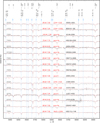 |
Fig. B.1. Spectra of all known UHE white dwarfs. The positions of photospheric lines (H I, He I, He II and C IV), α and β transitions between Rydberg states (n − n′) of the ionization stages V−X, and approximate line positions of the UHE features (blue) are marked. Overplotted in red are TMAP models and the effective temperatures, surface gravities, and chemical compositions (in mass fractions) as determined in previous works (see footnote of Table 1) or in the present study. The spectrograph used for the observation is indicated in gray. |
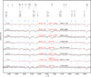 |
Fig. B.2. As in Fig. B.1 but for all known white dwarfs showing only the He II line problem but no UHE lines. |
All Tables
Names, spectral types, J2000 coordinates, observed Gaia eDR3 G band magnitudes, distances, Gaia extinction coefficients, dereddened Gaia color indexes, and the absolute dereddened G band magnitudes of all known UHE white dwarfs and white dwarfs showing only the He II line problem.
Predicted differences in the resulting magnitudes from synthetic spectra containing metals relative to a model containing only He.
Periods, mean magnitudes, and amplitudes as derived from various light curves for all periodically variable UHE white dwarfs.
Periods, mean magnitudes, and amplitudes as derived from various light curves for all periodically variable white dwarfs showing only the He II line problem.
Periods, mean magnitudes, and amplitudes as derived from ZTF DR4 light curves for all periodically variable normal hot white dwarfs.
All Figures
|
Fig. 1. Locations of the UHE white dwarfs (star symbols) and white dwarfs showing only the He II line problem (diamonds) in the Gaia HRD. Hot subdwarfs (triangles), SDSS white dwarfs (dots), and white dwarf–main sequence binaries (plus symbols) containing a very hot (Teff ≥ 50 000 K) white dwarf are also shown. The color coding indicates the effective temperatures of the stars. |
| In the text | |
|
Fig. 2. From left to right and top to bottom: target pixel files (TPFs) of WD 0101−182, J0146+3236, HS 0158+2335, J0254+0058, HS 0713+3958, HS 0727+6003, HS 0742+6520, HE 1314+0018, J1510+6106, and HS 1517+7403. The red circles are the sources of the Gaia catalog in the field with scaled magnitudes (see legend). Number 1 indicates the location of the targets. The aperture mask used by the pipeline to extract the photometry is also marked. |
| In the text | |
|
Fig. 3. Periodograms and phase-folded light curves of the UHE white dwarfs J0032+1604, WD 0101−182, J0146+3236, and HS 0158+2335. The red solid lines are phase-averaged light curves, while the dotted light curve represents the actual data. The black line is a fit of a harmonic series used to predict the peak-to-peak amplitude. |
| In the text | |
|
Fig. 4. As in Fig. 3 for the UHE white dwarfs J0254+0058, HS 0713+3958, HS 0727+6003, and J1059+4043. |
| In the text | |
|
Fig. 5. As in Fig. 3 but for the UHE white dwarfs J1215+1203, J1257+4220, HS 2027+0651, and HS 2115−1148. |
| In the text | |
|
Fig. 6. As in Fig. 3 but for the He II line problem white dwarfs J0821+1739 and J1029+2540, HE 1314+0018, and J1512+0651. |
| In the text | |
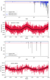 |
Fig. 7. As in Fig. 3 but for the He II line problem white dwarfs HS 1517+7403 and J1553+4832. |
| In the text | |
|
Fig. 8. Distribution of the photometric periods of the variable UHE and He II line problem white dwarfs (blue), and the period distribution of only the UHE white dwarfs (purple). On the left their period distribution is compared to the orbital period distribution of PCE CSPNe (light green; the bold teal line indicates the period distribution of binary CSPNe that show a reflection effect) and white dwarfs plus main sequence binaries (light yellow). Left panel: a comparison with the rotational periods of normal white dwarfs (light green with dashed contours) and magnetic white dwarfs (bold yellow lines). The median period and standard deviation of each sample is indicated. |
| In the text | |
|
Fig. 9. SDSS-ugriz light curves of J0254+0058. The solid line shows the light curve models using the parameters derived by fitting the SDSS-r light curve and a fixed albedo of A = 1 in all bands. The dashed lines give the light curve model fit that allows for unphysical variations in the albedo of the companion. |
| In the text | |
|
Fig. 10. Expected amplitude for J0254+0058 of the reflection effect as a function of the temperature of the heated side of the companion. The amplitude was calculated as the difference in flux of a white dwarf and a M-dwarf companion with the parameters derived in the light curve fit in phase 0 and phase 0.5 using a black-body approximation. |
| In the text | |
|
Fig. 11. Differences in the flux of models with different metal contents and a model containing only He (red). Upper panel: fluxes for different abundances of the iron-group elements, and lower panel: a model that contains opacities of He, C, and O. The filter response functions of the Galex FUV, NUV, and SDSS u, g, r, i, and z bands are indicated. |
| In the text | |
|
Fig. B.1. Spectra of all known UHE white dwarfs. The positions of photospheric lines (H I, He I, He II and C IV), α and β transitions between Rydberg states (n − n′) of the ionization stages V−X, and approximate line positions of the UHE features (blue) are marked. Overplotted in red are TMAP models and the effective temperatures, surface gravities, and chemical compositions (in mass fractions) as determined in previous works (see footnote of Table 1) or in the present study. The spectrograph used for the observation is indicated in gray. |
| In the text | |
|
Fig. B.2. As in Fig. B.1 but for all known white dwarfs showing only the He II line problem but no UHE lines. |
| In the text | |
Current usage metrics show cumulative count of Article Views (full-text article views including HTML views, PDF and ePub downloads, according to the available data) and Abstracts Views on Vision4Press platform.
Data correspond to usage on the plateform after 2015. The current usage metrics is available 48-96 hours after online publication and is updated daily on week days.
Initial download of the metrics may take a while.