| Issue |
A&A
Volume 647, March 2021
|
|
|---|---|---|
| Article Number | A102 | |
| Number of page(s) | 12 | |
| Section | Extragalactic astronomy | |
| DOI | https://doi.org/10.1051/0004-6361/202039984 | |
| Published online | 17 March 2021 | |
X-ray emission of Seyfert 2 galaxy MCG-01-24-12
1
Space Science Data Center, SSDC, ASI, via del Politecnico snc, 00133 Roma, Italy
e-mail: This email address is being protected from spambots. You need JavaScript enabled to view it.
2
INAF-Osservatorio Astronomico di Roma, via Frascati 33, 00078 Monteporzio Catone, Italy
3
Department of Physics and Astronomy – DIFA, University of Bologna, Via Gobetti 93/2, 40129 Bologna, Italy
4
European Space Agency (ESA), European Space Astronomy Centre (ESAC), 28691 Villanueva de la Cañada, Madrid, Spain
5
Dipartimento di Matematica e Fisica, Università degli Studi Roma Tre, via della Vasca Navale 84, 00146 Roma, Italy
6
INAF-Osservatorio Astronomico di Brera, Via Bianchi 46, 23807 Merate (LC), Italy
7
Department of Physics, Institute for Astrophysics and Computational Sciences, The Catholic University of America, Washington, DC 20064, USA
8
INAF/Istituto di Astrofisica e Planetologia Spaziali, via Fosso del Cavaliere, 00133 Roma, Italy
9
INAF-Osservatorio di Astrofisica e Scienza dello Spazio, via Gobetti 93/3, 40129 Bologna, Italy
10
ASI-Unità di Ricerca Scientifica, Via del Politecnico snc, 00133 Roma, Italy
Received:
24
November
2020
Accepted:
4
January
2021
Abstract
We present a detailed X-ray spectral analysis of the nearby Seyfert 2 galaxy MCG-01-24-12 based on a multi-epoch data set. Data were obtained with different X-ray satellites, namely XMM-Newton, NuSTAR, Swift, and Chandra, and cover different time intervals, from a few days to years. From 2006 to 2013 the source had a 2–10 keV flux of ∼1.5 × 10⁻¹¹ erg cm−2 s−1, consistent with archival observations based on HEAO and BeppoSAX data, though a 2019 Chandra snapshot caught the source in an extreme low flux state a factor of ∼10 fainter than its historical level. Based on phenomenological and physically motivated models, we find the X-ray spectrum of MCG-01-24-12 to be best modelled by a power-law continuum emission with Γ = 1.76 ± 0.09 with a high energy cut-off at Ec = 70−14+21 keV that is absorbed by a fairly constant column density of NH = (6.3 ± 0.5) × 1022 cm−2. These quantities allowed us to estimate the properties of the hot corona in MCG-01-24-12 for the cases of a spherical or slab-like hot Comptonising plasma to be kTe = 27−4+8 keV, τe = 5.5 ± 1.3 and kTe = 28−5+7 keV, τ = 3.2 ± 0.8, respectively. Finally, despite the short duration of the exposures, possible evidence of the presence of outflows is discussed.
Key words: galaxies: active / galaxies: Seyfert / X-rays: galaxies / X-rays: individuals: MCG-01-24-12
© ESO 2021
1. Introduction
Seyfert 2 galaxies are a class of active galactic nuclei (AGNs) whose optical spectra lack broad emission lines. These emission lines are not observed because the broad-line region (BLR) is hidden by matter with column density in the range 1022−24 cm−2 and because our line of sight passes through this obscuring circumnuclear medium, thought to be toroidal in structure. The so-called dusty torus absorbs and reprocesses (transmits and/or reflects) the X-ray nuclear continuum imprinting some characteristic features on the emerging spectrum. Although this obscuring structure is predicted to be ubiquitous in AGNs by the unification model (Antonucci 1993), there are still uncertainties on its exact location, composition, and overall geometry. In recent years both short- and long-term variability of the obscurer column density (NH) have been observed in nearby AGNs, such as NGC 1365 (e.g., Risaliti et al. 2005; Rivers et al. 2015), NGC 4388 (e.g., Elvis et al. 2004), NGC 4151 (Puccetti et al. 2007), and NGC 7582 (e.g., Piconcelli et al. 2007; Bianchi et al. 2009; Rivers et al. 2015; Braito et al. 2017), and changes in the column density have also been measured in heavily obscured AGN, for example NGC 1068 (e.g., Zaino et al. 2020). As a result, the standard picture of a smooth torus was ruled out in favour of a more inhomogeneous structure comprised of a distribution of a large number of individual clumps (e.g., Risaliti et al. 2002; Markowitz et al. 2014).
The high piercing power of X-rays, unless the obscuring matter has a column density larger than the inverse of the Thomson cross section ( cm−2), can allow the direct observation of the central regions where the primary X-rays originate (e.g., Nandra & Pounds 1994; Turner et al. 1997a; Guainazzi et al. 2005; Awaki et al. 2006). X-ray photons are produced by inverse-Compton scattering of disc optical-UV photons from thermal electrons, the so-called hot corona (details in Haardt & Maraschi 1991, 1993). Both variability and microlensing arguments (Chartas et al. 2009; Morgan et al. 2012; De Marco et al. 2013; Kara et al. 2016) agree that this hot plasma is compact and likely lies close to the SMBH. As expected on a theoretical basis, the physical quantities of the X-ray emitting region (its opacity and temperature) characterise the emerging spectrum in terms of photon index (Γ) and high energy cut-off (Ec; e.g., Rybicki & Lightman 1979; Ghisellini 2013). The relation between physical and phenomenological quantities has been the object of different studies (e.g., Beloborodov 1999; Petrucci et al. 2000, 2001; Middei et al. 2019). NuSTAR played a fundamental role in such a framework; due to its unrivalled capability of focusing X-rays up to about 80 keV, it allowed an increasing number of high energy cut-off measurements (e.g., Fabian et al. 2015, 2017; Tortosa et al. 2018), hence estimates of the coronal temperature (kTe) and optical depth (τe).
The primary X-ray continuum can be reflected off the black hole surroundings, and this emission may leave two major signatures on the emerging spectrum: a Fe Kα line at 6.4 keV due to fluorescence and a bump of counts at ∼30 keV (e.g., George & Fabian 1991; Matt et al. 1991), called the Compton hump.
Due to their variable emission, multi-epoch data sets are particularly suitable for studying AGNs spectral properties. In this context we report on the analysis of MCG-01-24-12, a bright spiral galaxy at redshift z = 0.0196 (e.g., Koss et al. 2011) hosting a Seyfert 2 nucleus (de Grijp et al. 1992). This AGN, first studied by Piccinotti et al. (1982) in the 2–10 keV band, was subsequently analysed by Malizia et al. (2002), who used BeppoSAX data to discuss its X-ray spectral properties. In particular, the source 2–10 keV band was characterised by a narrow Fe Kα emission line and an absorption feature at about 8 keV, while softer X-rays were absorbed by an obscurer with NH ∼ 7 × 1022 cm−2. In the hard X-ray band (20–100 keV) they measured a flux of ∼4 × 10⁻¹¹ erg cm−2 s−1. Later, MCG-01-24-012 was reported by Ricci et al. (2017) who used Swift data and measured its flux to be F14−195 keV = 4.1 × 10⁻¹¹ erg cm−2 s−1. Finally, the MCG-01-24-12 black hole mass was estimated to be MBH = 1.5 (La Franca et al. 2015).
2. Archival data
MCG-01-24-12 has been observed several times in the X-ray band. In Table 1 we present the log of the observations considered in this work.
Observation log of the presented data set.
The standard XMM-Newton Science Analysis System (SAS, Version 18.0.0) was used to obtain the scientific products for the different instruments on board the observatory, namely pn (Strüder et al. 2001) and the MOS cameras (Turner et al. 2001). To select the extraction radius and to screen for high background time intervals we used an iterative process that maximises the signal-to-noise ratio (S/N) (see details in Piconcelli et al. 2004). For the pn data, we used a 21 arcsec radius circular region to extract the source spectrum, and the background was computed with a circular area of 50 arcsec radius close to the source. The spectrum was then binned to have at least 30 counts for each bin, and to avoid oversampling the instrumental energy resolution by a factor larger than 3. Radii of 21 and 22 arcsec were adopted for MOS1 and MOS2, respectively, to extract the source spectrum, while we obtained the background using a circular area with 40 arcsec radius. The same binning strategy used for pn data was applied to the MOS spectra. We note that these XMM-Newton data are not affected by significant pile-up, this being in agreement with the SAS standard task epatplot. Moreover, we checked for any Cu emission possibly affecting the pn spectrum, and no evidence of it was found.
To calibrate and clean raw NuSTAR data we used the NuSTAR Data Analysis Software (NuSTARDAS, Perri et al., 20131) package (v. 1.8.0). Level 2 cleaned products were obtained with the standard nupipeline task, and the scientific products were computed thanks to the nuproducts pipeline and using the calibration database 20191219. A circular region with a radius of 40 arcsec was used to extract the source spectrum. The background was calculated using the same circular region but centered in a blank area near the source. The FPMA/B spectra were binned in order not to oversample the instrumental resolution by a factor larger than 2.5 and to achieve a S/N higher than 3 in each spectral channel.
Swift-XRT data were taken in photon counting mode and we derived the scientific products using the facilities provided by the Space Science Data Center (SSDC2) of the Italian Space Agency (ASI). The source spectrum was extracted with a circular region of ∼60 arcsec and we used a concentric annulus for the background. The spectra were then binned in order to have at least 20 counts in each bin. Due to their short exposures we do not show the XRT light curves.
An exposure of approximately 10 ks of MCG-01-24-12 was carried out by Chandra on 27 June 2019 with the Advanced CCD Imaging spectrometer (ACIS-S; Garmire et al. 2003). The data were reduced by adopting the Chandra Interactive Analysis of Observation software (CIAO v. 4.12 Fruscione et al. 2006) and the latest Chandra Calibration Data Base (CALDB version 4.9.2.1). The source and background spectra were extracted using a circular region of 2.5″ and 4.0″ radius, respectively. Furthermore, the resulting spectrum was re-binned by a minimum of 20 counts per energy bin and with a total net count of 610 for a net exposure time of 9133 s.
In all the fits of simultaneous Swift-NuSTAR observations the inter-calibration between the different NuSTAR modules and the Swift X-ray telescope is taken into account by a cross-normalisation constant. The FPMA/B modules were always found consistent within 3%, with the exception of observation 1 where they agree within 30%. In particular, the FPMB spectrum has about 1000 counts more than FPMA/B. In this latter module, the source was found to lie between the detector chips, which explains the decreased number of photon counts. However, by fitting individually the FPMA/B spectra with an absorbed power law the returned photon indices were consistent within the errors, hence we decided to include data from both modules in the analysis. In all but one pointing Swift/XRT and NuSTAR are consistent within ≲10%, in agreement with Madsen et al. (2015). On the other hand, for observation 4 we obtained const = 1.5 ± 0.3 as NuSTAR caught the source in a higher flux state than the shorter Swift snapshot. For a quick comparison of the data, we show all the data in Fig. 1. Finally, MOS1 and MOS2 are consistent with pn data within 3%.
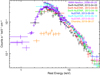 |
Fig. 1. MCG-01-24-12 spectra as observed by the different observatories, and folded by a power law with Γ = 2 and unitary normalisation. |
We preliminarily computed the MCG-01-24-12 light curves for the NuSTAR data. In Fig. 2 we report the corresponding time series in various bands (as labelled on the y-axis), while in the last row we show the ratios of the 3–10 to the 10–79 keV bands. X-ray variability is typical of AGNs, and it has been measured on timescales ranging from kiloseconds to decades (e.g., Green et al. 1993; Uttley et al. 2002; Vagnetti et al. 2011, 2016; Ponti et al. 2012; McHardy et al. 2007; Middei et al. 2017; Paolillo et al. 2017). Regarding MCG-01-24-12, observation 2 varies by a factor of 50% in the 3–10 keV energy band over a few kiloseconds, while the other exposures have a more constant behaviour in the same energy band. On the other hand, variations are witnessed when comparing light curves at different observing epochs. The maximum amplitude change, about a factor of 2, occurred in the 3–10 keV energy band on a timescale of about 1 month (between observations 1 and 6). The ratios of the 3–10 keV to the 10–79 keV bands have a rather constant behaviour, with the exception of observation 2 in which the source hardness increased as the flux decreased. However, the short exposure does not allow us to perform a time-resolved spectral analysis of observation 2, hence we used the time-averaged spectra to improve the fit statistics of all the observations. All errors reported in the plots account for 1σ uncertainty, while errors in text and tables are quoted at the 90% confidence level.
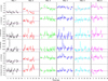 |
Fig. 2. Background subtracted NuSTAR light curves of MCG-01-24-12 calculated with a temporal bin of 1000 s. Light curves account for co-added module A and B, and the various energy bands are labelled on the y-axis. For each observation a specific colour is used; this colour-coding is adopted throughout the whole paper. The horizontal straight lines are used to quantify the average count rate within each observation for the different bands, while dashed lines account for 1σ uncertainties around the mean. |
3. Spectral analysis
We used XSPEC (Arnaud 1996) to fit the data with the Galactic column density kept frozen to the value NH = 2.79 × 1020 cm−2 (Ben Bekhti 2016). Moreover, the standard cosmology ΛCDM (H0 = 70 km s−1 Mpc−1, Ωm = 0.27, Ωλ = 0.73) is adopted throughout the analysis.
3.1. Epic camera view: 0.3–10 keV band
We started studying the 0.3–10 keV EPIC data using a simple model (const×tbabs×ztbabs×power-law, in XSPEC notation) whose components account for the inter-calibration between the cameras, the Galactic absorption, the MCG-01-24-12 intrinsic absorption, and its primary continuum emission. This model leaves prominent residuals in the soft X-ray band, and the fit is unacceptable on statistical grounds (χ2 = 355 for 243 d.o.f.). The excess in the soft X-rays may be due to a fraction of the coronal primary emission that is scattered or reflected possibly by distant material. This behaviour in obscured AGNs is quite typical. This energy band is generally dominated by emission lines from a photonionised gas coinciding with the narrow-line region (NLR; e.g., Bianchi et al. 2006; Guainazzi & Bianchi 2007), though the lack of high statistics or the low resolution of X-ray spectra makes it possible to model such a component with a simple power law (e.g., Awaki et al. 1991; Turner et al. 1997a,b). Since our spectra do not show any of these features, we model the scattered component in the EPIC data adding an additional power law. A test fit showed the photon indices of the power laws accounting for the primary X-ray continuum and the scattered emission to be compatible within the errors, hence in the following fits we linked these parameters. The normalisation of the scattered component was fitted and found to be a few percent of the primary continuum (e.g., Bianchi & Guainazzi 2007). The addition of this new component is beneficial in terms of statistics, and the fit improved by Δχ2/Δd.o.f. = −83/−1.
Residuals are still visible in the Fe Kα band, and are reported in the top panel of Fig. 3 and further supported by the blind line scan shown in the bottom panel of the same figure. The blind line scan was carried out by using an absorbed power law and a Gaussian model with a fixed line width of 1 eV (i.e. much lower than the CCD resolution) with line energy allowed to vary in the range 5 − 10 keV and normalisation from −6 × 10⁻⁵ to 10−4 ph. keV−1 cm−1 s−1 with 50 steps. This test suggests the presence of a strong Fe Kα emission line at the rest-frame energy of E = 6.39 ± 0.05 keV and an absorption trough at ∼ 7.4 ± 0.1 keV at the ∼5σ and ∼3σ confidence levels, respectively. We accounted for these features by adding two Gaussian components, one for reproducing the Fe Kα feature, the other the trough above ∼7 keV. For both these components we fitted the line’s energy centroid, its width, and its normalisation. Since we only get an upper limit for the width of the absorption component σFe K < 160 eV, we fixed this parameter to this value. The addition of the Gaussian emission improved the overall statistic by Δχ2 = 18 for 3 d.o.f. less, while a Δχ2/Δd.o.f. = −10/−2 corresponds to the line in absorption. The described procedure led to a best fit of χ2 = 243 for 237 d.o.f. for which we report best-fit parameters in Table 2. The EPIC spectra are therefore well described by a power-law continuum (Γ = 1.68 ± 0.04) absorbed by an obscurer with column density of NH = 6.4 ± 0.3 × 1022 cm−2. The continuum is accompanied by a moderately broad (σ = 80 ± 60 eV) neutral Fe emission line and a weak absorbing signature. Finally, the soft X-ray band is dominated by a fraction of the primary continuum scattered (see Fig. 4).
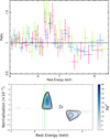 |
Fig. 3. Top panel: ratio of the EPIC spectra in the 5–8.5 keV energy range with respect to an absorbed power law. All the instruments (pn in blue, MOS1 in magenta, and MOS2 in green) detected the Fe Kα and found a trough at about 7.5 keV. Bottom panel: blind line scan result between the normalisation and line energy, adopted on the pn-MOS spectra, where a Gaussian is left free to vary in the 5–8.5 keV energy range. The colour bar on the right indicates the significance of the lines for 2 degrees of freedom and the solid black contours correspond to 68%, 90%, and 99%. |
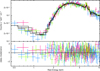 |
Fig. 4. Best-fit model to the EPIC-pn&MOS with a corresponding statistics of χ2 = 243 for 237 d.o.f. |
3.2. Broad-band Swift/NuSTAR view I: Phenomenological model
We started analysing the NuSTAR data by fitting each observation separately with an absorbed power law and the corresponding residuals are shown in Fig. 5. To better quantify the possible variability of the Fe Kα and to further investigate for the presence of any additional features, we performed a blind line scan over the spectra. The line scan procedure was the same described for the XMM-Newton data. The resulting contour plots are reported in Fig. 6. The Fe Kα line appears stronger in observations 2 and 6, while it is only marginally detected in all the remaining pointings. Interestingly, in observation 6 the energy spectrum suggests the presence of an absorbing signature above ∼7 keV. A fit of such a feature with a narrow Gaussian component returns E = 7.35 ± 0.10 keV, N = (1.8 ± 0.8) × 10−5 ph. cm−2 s−1 and EW = − 80 ± 35 eV, with an improvement of the fit statistics of Δχ2/d.o.f. = −14/−2. We then also considered the Swift data, and fitted the Swift-NuSTAR observations using a Gaussian line to account for the Fe Kα emission plus an absorbed cut-off power law to reproduce the continuum, written in XSPEC syntax as tbabs×ztbabs×(cutoffpl+zgauss). The high energy cut-off for the primary emission is included in order to model the counts drop observed above ∼40 keV in Fig. 5 for observations 3, 5, and 6. The current data, with observation 6 being a possible exception, does not allow an appropriate characterisation of the troughs in the spectra, thus we did not account for them in the modelling. The fitting procedure was performed allowing the photon index, the high energy cut-off, and the continuum normalisation to vary in each observation. Then we calculated the emission line normalisation, while the energy centroid was set to 6.4 keV. We assumed the line to have a narrow profile with sigma fixed to 1 eV. After a preliminary fit showing the obscurer column density to be consistent within the uncertainties in all the pointings, we tied the ztbabs between the different observations. The Swift-XRT data have too poor statistics to constrain any scattered emission (see Fig. 1), and for this reason we do not include an additional power law accounting for such a component. This fit leads to a fit characterised by χ2/d.o.f. = 1309/1256, and in Table 3 we quote the corresponding best-fit parameters.
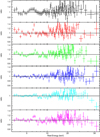 |
Fig. 5. Data/model ratios of the NuSTAR FPMA/B spectra. The underlying model accounts for an absorbed power law const×tbabs×ztbabs×po for each observation. |
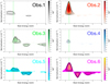 |
Fig. 6. Result of a blind line scan performed to all six NuSTAR observations plotted between the 5.5 − 10 keV band. The colour bar on the right of each panel indicates the significance of the lines for 2 degrees of freedom and the solid black contours correspond to 68%, 90%, and 99%. The lime green vertical dashed line indicates the position of the rest frame energy of the Fe Kα emission line at E = 6.4 keV. |
Swift-NuSTAR best-fit parameters derived using an absorbed power law plus a Gaussian component accounting for the Fe Kα emission line (tbabs×ztbabs×(zgauss+power-law) in XSPEC) corresponding to Δχ2/d.o.f. = 1309/1256.
The current phenomenological model is consistent with a power law with constant shape that is absorbed by an average column density NH = (6.6 ± 0.4) × 1022 cm−2. Moreover, the Fe Kα emission line, assumed to have a narrow intrinsic profile, seemed to be variable, at least in observations 2 and 6. To further assess the actual variability of this component, we assumed the emission line flux to be the same over the whole campaign. In other words, starting from the phenomenological best fit, we fitted the data tying the Fe Kα normalisation between the observations. The obtained fit has worse statistics (Δχ2/Δd.o.f. = +23/+5), thus further supporting the line to be variable with significance greater than 95%.
3.3. Broad-band Swift/NuStar view II: Reflection signature with xillver
As a subsequent step we studied the XRT-FPMA/B spectra using xillver (e.g., García et al. 2014; Dauser et al. 2016), a model that self-consistently calculates the underlying nuclear emission (a cut-off power law) and the reflected component from the illuminated accretion disc. Then we left free to vary and compute in each observation the photon index, the reflection parameter R, and the model normalisation. We considered the reflecting matter to be nearly neutral, we fixed the ionisation parameter log ξ to a value of 0, and we calculated the Fe abundance (AFe) linking its value between the different observations. Though we know the ztbabs component does not vary significantly during the monitoring, we fitted this component in all the observations. These steps led to the best-fit parameters in Table 4 and characterised by a statistic of χ2/d.o.f. = 1252/1258, see Fig. 7. The overall fit is consistent with a primary emission continuum absorbed by an average column density of NH = (6.3 ± 0.5) × 1022 cm−2 and the reflecting matter arising from a cold disc region with a solar metal abundance AFe = 1.3 ± 0.6. The photon index of the primary continuum varies in the range 1.68–1.93, though the obtained best-fit values are consistent within the uncertainties. In a similar fashion, marginal variability is observed for the high energy cut-off and the reflection parameter and, as expected from the light curves in Fig. 2, the normalisation of xillver is found to vary. We list the best-fit parameters in Table 4; the contour plot referring to the photon index, the reflection fraction, and the high energy cut-off are shown in Fig. 8.
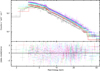 |
Fig. 7. Best fit (χ2/d.o.f. = 1252/1257) to the simultaneous Swift-NuSTAR data obtained using xillver. |
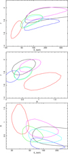 |
Fig. 8. Contours at 90% confidence level (Δχ2 = 4.61 for two parameters) between the photon index Γ and the high energy cut-off (Ec, top panel) and the reflection fraction (middle). Contours in the bottom panel refer to the high energy cut-off and the reflection fraction. All the contours have been computed with the column density, the photon index, the high energy cut-off, the reflection fraction, and the xillver normalisation free to vary in all the observations. |
Swift-NuSTAR best-fit values derived using tbabs×ztbabs×xillver in XSPEC notation and that corresponds to a statistic χ2/d.o.f. = 1252/1257.
We further tested the data using the same model but tying the photon index, the reflection fraction, the high energy cut-off, and the column density of the obscurer between the exposures. The fit returns a statistic of χ2 1300 for 1278 d.o.f., not far from the previous value, and further supports a weak variability of the parameters.
3.4. Broad-band Swift/NuStar view III: Reflection signature with MyTorus
In the above fitting (Sect. 3.3) xillver assumes a geometrically simple slab reflector. Therefore, as an alternative scenario, we replaced both the xillver and the simple neutral absorber (ztbabs) with MyTorus (Murphy & Yaqoob 2009). This model takes into account the physical properties of the absorbing medium such as its toroidal geometry and the Compton down-scattering effect, and it includes self-calculated reflected components (continuum plus Fe K emission lines). The overall MyTorus model adopted here is composed of three publicly available tables (two additive and one multiplicative), developed for XSPEC, which self-consistently compute the reflected continuum (MyTorusS), the Fe Kα, Fe Kβ fluorescent emission lines (MyTorusL) and the zeroth-order line-of-sight attenuation (MyTorusZ). The model assumes a fixed geometry of the toroidal X-ray reprocessor, a single value for the covering factor of the torus corresponding to a half-opening angle of 60°.
We first constructed the MyTorus model according to the ‘coupled’ solution (Yaqoob 2012), where our line-of-sight angle that intercepts the torus is directly co-joined (or coupled) to the scattered angle. In other words, it is assumed that the fluorescent and reflected emissions emerge from the same medium that is also responsible for the line-of-sight attenuation of the X-ray underlying continuum. Thus, we set the column density of each MyTorusS, MyTorusL, and MyTorusZ grid to be the same within each observation but free to vary between the six pointings, whilst their normalisations are linked with that of a power law accounting for the primary continuum. In a similar fashion, the photon index of the three grids was linked with the nuclear index that was computed for each observation. These steps lead to a fit to the data of χ2/d.o.f. = 1316/1255, and considerably improves (by Δχ2/Δd.o.f. = − 25/+1) once the viewing inclination angle (θobs, kept constant between the observations) is measured. However, the returned value of line-of-sight inclination angle is  deg, just at the extremity of the MyTorus parameter space (i.e. θobs = 60 deg).
We then considered a more complex morphology (i.e. clumpy medium), MyTorus further allows us to test a scenario in which the reflected and the transmitted components emerge from matter with different column densities (decoupled solution; see Yaqoob 2012, for more details) in a system characterised by a more patchy distribution of reprocessing clumps. In this configuration our line of sight might intercept the transmitted (or zeroth-order) component through one region of the torus and the reflected emission that is back scattered from a different location of the torus itself (see Yaqoob 2012, Fig. 2). This solution was obtained by decoupling the inclination parameter (θobs) of the zeroth-order (i.e. line of sight) and reflected table components with respective column densities defined as NH, Z (line-of-sight NH ) and NH, S (global NH). The corresponding inclination parameters are fixed at θobs, Z = 90° and θobs, S = 0° for the zeroth-order and reflected continua components, respectively. In this scenario we find that the global column density is much larger than the zeroth-order measured at  , and the corresponding best-fit data is shown in Fig. 9. Such a model is in agreement with an emission spectrum that is nearly Compton-thick out the line of sight and Compton-thin along the line of sight. The decoupled configuration yielded a χ2 = 1274 for 1258 d.o.f.; see Table 5 for the corresponding MyTorus best-fit values. This result also suggests that the overall column density of the torus might be inhomogeneous in nature, and indeed the upper parts are less dense than the central one.
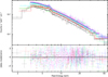 |
Fig. 9. Simultaneous Swift-NuSTAR observations fitted using MyTorus in its decoupled configuration (χ2/d.o.f. = χ2 = 1274 for 1258 d.o.f.). |
Swift-NuSTAR best-fit values for the parameters obtained using the decoupled MyTorus solutions.
3.5. Joint XMM-Newton, Swift, and NuSTAR data
The lack of substantial spectral variability between the XMM-Newton pointing and the 2013 monitoring campaign encouraged us to perform a broad-band fit based on all these data. Therefore, we simultaneously tested the two physically motivated models in Sects. 3.3 and 3.4 on the entire data set, i.e. on the XMM-Newton, Swift and NuSTAR spectra.
We started using xillver for which we fitted the photon index, the high energy cut-off, and the reflection fraction linked between the pointings. We also included the scattered power-law component for which we only fitted the normalisation as its photon index was linked to the xillver normalisation. To account for the flux variability we used a constant free to vary in all but the XMM-Newton exposure in which the xillver normalisation was computed instead. This procedure returned a fit with statistic χ2 = 1528 for 1508 degree of freedom. The best-fit parameters were consistent with those previously found: NH = (6.6 ± 0.2) × 1022 cm−2, Γ = 1.75 ± 0.05, Ec = 70 ± 15 ± keV, AFe = 1.5 , R = 0.45 ± 0.15, and the constant varied in the range 1.04–1.95.
Then we tested the decoupled solution of MyTorus. We fitted the data as we reported previously (see Sect. 3.4), and we used a free-to-vary constant to account for the variations in the different observations. As we did for the case of xillver, we also added a scattered power law. These steps yielded a χ2 = 1559 for 1510 d.o.f. for which the derived best-fit quantities are consistent with those quoted in Table 5.
These tests further point towards a fairly constant behaviour of the primary continuum shape and the absorbed component in MCG-01-24-12, at least for the data from 2006 to 2013. Although the ionised reflection model is somewhat preferred in terms of the fit statistic, both the xillver and MyTorus solutions give good fits. In Fig. 10 we report the best-fit data and the corresponding underlying model for the cases of xillver and MyTours.
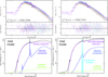 |
Fig. 10. Left panels: XMM-Newon/Swift/NuSTAR best-fit data using xillver (top). The different spectral components are reported in the corresponding bottom graph. Right panels: XMM-Newon/Swift/NuSTAR best-fit data (top) and model components (bottom) corresponding to the decoupled MyTorus solution. |
As a final test, we modelled the absorption trough at ∼7.4 keV on the complete data set. In particular, we used an XSTAR (Kallman et al. 2004) table assuming an input spectrum of Γ = 2 across the 0.1–106 eV band and a high energy cut-off at Ec = 100 keV. The elemental abundance was set to solar (Asplund et al. 2009), and we assumed a velocity broadening vturb = 5000 km s−1 and the absorber to be fully covering. In the fit we allowed the absorber’s column density, ionisation state, and redshift to vary and we tied these parameters between the different observations. This additional component improved the fit with Δχ2/Δd.o.f. = −11/−3, with NH = (2.3 ) × 1022 cm−2, log(ξ/erg cm−2s−1) > 3.1, and zobs = −0.075 ± 0.030 (corresponding to a velocity vxstar = −0.097 ± 0.032). However, as suggested in Fig. 6 this absorption feature seemed to be more prominent in observation 6. For this reason we unlinked and fitted the absorber parameters in this observation, and found an additional enhancement of the fit statistics (Δχ2/Δd.o.f. = −13/−3). The derived best-fit values are consistent with each other as we obtained NH = (1.3
 ) × 1023 cm−2, log(ξ/erg cm−2s−1) = 3.2 ± 0.4 for zobs = −0.076 ± 0.018. Untying these parameters across all the observations would lead to a marginal improvement of Δχ2/Δd.o.f. = −21/−15. Finally, these values are fully compatible with each other and with the parameters commonly measured for these absorbers in other AGNs (e.g., Gofford et al. 2013; Tombesi et al. 2013).
3.6. The 2019 ACIS/S spectrum
The poor statistics of the Chandra snapshot did not allow us to do a detailed spectral analysis. A simple phenomenological model such as an absorbed power law failed to reproduce the hard continuum and returned a photon index Γ ≲ 1. Then we tested a scenario in which the source had an intrinsic flux drop likely due to a change in its luminosity. To do this we applied the best-fit model used for the EPIC data (see Table 2) on the Chandra spectrum and we refit this data only allowing the primary normalisation to vary. This procedure yielded a fit with χ2 = 56 for 29 d.o.f. and returned a primary normalisation Npo = (7.0 ± 0.5) × 10−4 ph. keV−1 cm−2 s−1 and an observed flux F2−10 keV = (2.15 ± 0.15) × 10−12 erg cm−2 s−1, a factor of 10 lower than previously measured. This intrinsic flux drop seems to be favoured with respect to a scenario in which the NH of the neutral obscurer changed: keeping the normalisation of the primary power law fixed to the best-fit value (see Table 2) and letting free to vary only the column density of the neutral obscurer returned a χ2/d.o.f. > 11. A simultaneous fit of both the primary continuum normalisation and the obscuring column led to a fit statistic of χ2/d.o.f. = 53/28 with NH = 7.4 ± 1.0 × 1022 cm−2 and Npo = (7.5 ± 0.8) × 10−4 ph. keV−1 cm−2 s−1. The fit of the Fe Kα energy centroid normalisation enhanced the fit by Δχ2/Δd.o.f. = −12/−2. The Fe Kα has energy E = 6.5 ± 0.1 keV, normalisation NFe Kα = (1.1 ± 0.8) × 10−5 ph. cm−2 s−1, and EW = 320 ± 230 eV, which are consistent within the errors with what was previously observed. The limited bandwidth of the data did not allow us to further investigate the presence of any absorption features nor to firmly determine the physical origin of such a low flux state.
4. Discussion and conclusions
We reported on the X-ray emission properties of the Seyfert 2 galaxy MCG-01-24-12 based on observations taken with several X-ray facilities over a time interval spanning about 13 years. In the following we summarise and discuss our findings.
4.1. Variability and phenomenological modelling
XMM-Newton and NuSTAR data are consistent with a moderate variability of the source flux in the 3–10 keV band with values in the range of 1.2–2.3 × 10⁻¹¹ erg cm−2 s−1. Interestingly, this flux state is consistent with what was measured using BeppoSAX data (Malizia et al. 2002) and by Piccinotti et al. (1982).
We computed the bolometric luminosity and Eddington ratio of the source assuming an average flux state which corresponds to a luminosity L2−10keV ∼ 1.5 × 1043 erg s−1. Following the prescription in Duras et al. (2020) and using a SMBH mass MBH = 1.5 × 10⁷ M⊙ (La Franca et al. 2015), we derived LBol ∼ 1.9 × 1044 erg s−1 and LBol/LEdd ∼ 11%, respectively. As displayed in Fig. 2, variations occurred on weekly timescales, and intra-observation changes are weak, with the only exceptions being observations 2 and 3 where the hardness ratios also suggest some spectral change down to kilosecond timescales. On the other hand, the 2019 exposure performed with Chandra caught the source in an unprecedentedly observed faint state (L2−10keV ∼2 × 1042 erg s−1 ). The source faded by a factor of ∼10 from the last NuSTAR exposure. Different physical origins explained remarkable variations in other AGNs: (i) an increase in the neutral obscuration where the column density swings from Compton-thin to -thick on timescales of hours to days, as seen in the prototype changing-look AGN NGC 1365 (see Risaliti et al. 2005; ii) an obscuration event due to the clumpy highly ionised disc wind, as seen in MCG-03-58-007 (Braito et al. 2018; Matzeu et al. 2019; iii) strong intrinsic variability but neutral NH that is fairly constant, as in the case of NGC 2992 discussed in Murphy et al. (2007) and Middei et al. (in prep.).
From a phenomenological prospective, the primary emission of MCG-01-24-12 is consistent with an absorbed power law where the column density and spectral shape had a fairly constant behaviour within the NuSTAR monitoring, and when these 2013 data are compared with those from XMM-Newton and BeppoSAX. The Fe Kα emission line seems to vary in the NuSTAR spectrum and is strongly detected in observations 2 and 6. In this respect, we note that the strongest Fe Kα is in observation 2 (see Table 3 and Fig. 6) and that the line flux seems not to follow the weak variations of the continuum. This behaviour can be explained by the reverberation of the Fe Kα line (see e.g., Zoghbi et al. 2019) that, produced in a distant region such as the BLR, would have a delayed response with respect to the primary continuum.
The short duration of the exposures coupled with the instrumental spectral resolution prevented a detailed analysis of the line profile that was set to be narrow. On the other hand, the EPIC data are consistent with a moderately broad Fe Kα emission line (σ = 80 ± 60 eV) corresponding to a region of some hundredths of a parsec3. Interestingly, troughs above 7 keV have been observed in both NuSTAR and XMM-Newton spectra, possibly suggesting the presence of fast and highly ionised outflows.
4.2. Physically motivated modelling
Xillver provided the best fit to the Swift-NuSTAR data, specifically a cut-off power-law continuum plus its associated Compton reflected spectrum absorbed by a column density of about (6.3 ± 0.5) × 1022 cm−2. The chemical abundance of the reflecting material is consistent with being solar (AFe = 1.3 ± 0.6), and the continuum photon index, high energy cut-off, and reflection fraction are constant within the errors in all but observation 2 (see Fig. 8). This observation is the only one characterised by a variable ratio of the 3–10 and 10–79 keV light curves, and this possibly explains the discrepancies between observation 2 and the other observations. Such a case of short-term spectral variability is quite peculiar for MCG-01-24-12 since the analysis of the other exposures agrees with an intra-observation constancy of the primary photon index. Moreover, a fit performed with the photon index, the high energy cut-off and the reflection fraction linked between the observations returns a statistic of χ2 = 1300 for 1278 d.o.f. and the best-fit parameters are consistent with those computed by fitting the observations separately.
For this reason, we used the average values for the photon index (Γ = 1.76 ± 0.09) and the high energy cut-off ( keV, values also consistent with those found in Baloković et al. 2020) to derive the properties of the hot corona. The physical conditions of the emitting plasma are indeed responsible for the spectral shape and the high energy curvature of the X-ray continuum (e.g., Rybicki & Lightman 1979; Beloborodov 1999; Petrucci et al. 2000, 2001; Ghisellini 2013; Middei et al. 2019). The relations between Γ − Ec and kTe − τe have been recently derived by Middei et al. (2019) who used extensive simulations computed with the Monte Carlo code for Comptonisation in Astrophysics (MoCA; Tamborra et al. 2018) to study the Comptonised spectrum of AGNs (see also Marinucci et al. 2019; Lanzuisi et al. 2019, for further applications of this code). In particular, using Eqs. (2)–(5) in Middei et al. (2019), we found the hot corona in MCG-01-24-12 to be characterised by kTe = 27
 keV, τe = 5.5 ± 1.3 and kTe = 28
 keV, τ = 3.2 ± 0.8 for a spherical emitting plasma and a slab-like one, respectively. These values are fully in agreement with the average temperature and opacity values found in the literature (e.g., Fabian et al. 2015, 2017; Tortosa et al. 2018; Middei et al. 2019). Then we used the coronal temperature and opacity to include this source in the compactness–temperature l − θe) diagram (e.g., Fabian et al. 2015, 2017). We calculated the dimensionless coronal temperature θe = kTe/mec2 and the compactness parameter l = LσT/Rmec3, in which L accounts for the coronal luminosity in the 0.1–200 keV band and R for its radius that is assumed to be 10 gravitational radii (R10). Following these prescriptions, we derived θe = 0.053
 and l ≃ 55. These values are in agreement with the bulk of measurements presented by Fabian et al. (2015), and show that the source lies in the so-called permitted region where annihilation is still dominant with respect to the pair production.
We find MyTorus can provide a good representation of the Swift-NuSTAR data. Although the coupled solution is not adequate to described the overall spectrum of MCG-01-24-12 (with this mainly due to the relatively small curvature at low energies of NuSTAR data and the poor statistic of XRT spectra), the decoupled configuration provides a statistically acceptable representation of the Swift-NuSTAR spectra of MCG-01-24-12. We measured a considerable difference between the column densities of the global (out of the line of sight) and transmitted reprocessors. The nuclear radiation is absorbed by a neutral medium with the column density NH, Z in the range (5.3–11.7) × 1022 cm−2 and the reflected component is back mirrored by matter with global NH, S = 1.3 cm−2. This distinction between the zeroth-order and the global density has already been observed in other Seyfert 2 galaxies, for example NGC 4945 (Yaqoob 2012), Mrk 3 (Yaqoob et al. 2015), MCG-03-58-007 (Matzeu et al. 2019), NGC 4507, and NGC 4347 (Kammoun et al. 2019), and is described further in Kammoun et al. (2020). Thus, the emerging picture is consistent with an overall inhomogeneous or patchy toroidal absorber, broadly Compton-thin, with a distribution of relatively small and thicker equatorial clouds out of the line of sight. In most recent torus models the ‘viewing probability’ of the absorber, which is strongly correlated with its size and location, tend to be typically distributed towards the equatorial plane. The inhomogeneous gas distribution of the torus is now a well-established scenario within the scientific community, where a variety of models have been developed in order to take into account this physical framework (e.g., Elitzur & Shlosman 2006; Nenkova et al. 2008a,b; Tanimoto et al. 2019).
4.3. Is there a variable wind in MCG-01-24-12?
The inhomogeneous nature of the absorber and a viewing angle that possibly just passes through a semi-transparent obscurer allowed us to observe the nuclear regions of the MCG-01-24-12. This framework was found suitable for the star-forming galaxy MCG-03-58-007 (Braito et al. 2018). This source hosts a very powerful (vout ∼ 0.1−0.3 c), variable (δt ≲ 1 day), and multi-structured disc wind launched between tens to hundreds of gravitational radii from the black hole (see Matzeu et al. 2019, Fig. 9). The possible detection of blue-shifted absorption lines on XMM-Newton and NuSTAR observation 6 spectra may suggest MCG-01-24-12 to be similar to MCG-03-58-007. If the absorption troughs are associated with Fe XXVI Lyα they would correspond to a highly ionised gas outflowing at vout ∼ (0.06 ± 0.01)c4. Interestingly, in accordance with the blind line scan, the absorption feature above ∼7 keV has a significance ≳90% in three NuSTAR observations and in the XMM-Newton observation. These troughs, together with the one found by Malizia et al. (2002) in the BeppoSAX/PDS data, may suggest the presence of a persistent wind. We finally note that a powerful disc wind has been invoked to explain the low flux state observed in MCG-03-58-007 (Braito et al. 2018; Matzeu et al. 2019) where the authors found the source variability to be caused by a highly ionised fast wind rather than by a neutral clumpy medium. The low counts of the Chandra snapshot did not allow us to test this scenario, and a longer XMM-Newton exposure is needed to confirm the putative outflow in MCG-01-24-12 and to further understand the physics behind its low flux state. Moreover, future observations through the high resolution micro-calorimeter detectors on board XRISM and ATHENA will provide unprecedented details of these obscuration events.
This approximate estimate is derived via the virial theorem from which the Fe Kα emission line originates at r = (E/ΔE)2 × rg. In our case this estimate returns r ∼ 1.4 × 1016 cm.
This outflowing velocity has been derived following vzabs = ((1+zabs)2−1)/((1+zabs)2+1) and vout/c = (u−vzabs)/(1−(uvzabs)), where zabs is the redshift of the feature and u is the systemic velocity of MCG-01-24-12.
Acknowledgments
We thank the anonymous referee for useful comments. R. M. thanks Fausto Vagnetti for discussions and insights and Francesco Saturni for useful comments. RM acknowledges the financial support of INAF (Istituto Nazionale di Astrofisica), Osservatorio Astronomico di Roma, ASI (Agenzia Spaziale Italiana) under contract to INAF: ASI 2014-049-R.0 dedicated to SSDC. Part of this work is based on archival data, software or online services provided by the Space Science Data Center – ASI. S. B. acknowledges financial support from ASI under grants ASI-INAF I/037/12/0 and ASI-INAF n.2017-14-H. A.D.R. acknowledges financial contribution from the agreement ASI-INAF n.2017-14-H.O. S. B., A. D. R., M. D., A. M. and A. Z. acknowledge support from PRIN MIUR project “Black Hole winds and the Baryon Life Cycle of Galaxies: the stone-guest at the galaxy evolution supper”, contract no. 2017PH3WAT. Part of this work is based on archival data, software or online services provided by the Space Science Data Center – ASI. This work is based on observations obtained with: the NuSTAR mission, a project led by the California Institute of Technology, managed by the Jet Propulsion Laboratory and funded by NASA; XMM-Newton, an ESA science mission with instruments and contributions directly funded by ESA Member States and the USA (NASA).
References
- Antonucci, R. 1993, ARA&A, 31, 473 [Google Scholar]
- Arnaud, K. A. 1996, in Astronomical Data Analysis Software and Systems V, eds. G. H. Jacoby, & J. Barnes, ASP Conf. Ser., 101, 17 [Google Scholar]
- Asplund, M., Grevesse, N., Sauval, A. J., & Scott, P. 2009, ARA&A, 47, 481 [NASA ADS] [CrossRef] [Google Scholar]
- Awaki, H., Koyama, K., Inoue, H., & Halpern, J. P. 1991, PASJ, 43, 195 [NASA ADS] [Google Scholar]
- Awaki, H., Murakami, H., Ogawa, Y., & Leighly, K. M. 2006, ApJ, 645, 928 [NASA ADS] [CrossRef] [Google Scholar]
- Baloković, M., Harrison, F. A., Madejski, G., et al. 2020, ApJ, 905, 41 [Google Scholar]
- Beloborodov, A. M. 1999, in High Energy Processes in Accreting Black Holes, eds. J. Poutanen, & R. Svensson, ASP Conf. Ser., 161, 295 [Google Scholar]
- Bianchi, S., & Guainazzi, M. 2007, in The Multicolored Landscape of Compact Objects and Their Explosive Origins, eds. T. di Salvo, G. L. Israel, L. Piersant, et al., Am. Inst. Phys. Conf. Ser., 924, 822 [Google Scholar]
- Bianchi, S., Guainazzi, M., & Chiaberge, M. 2006, A&A, 448, 499 [NASA ADS] [CrossRef] [EDP Sciences] [Google Scholar]
- Bianchi, S., Piconcelli, E., Chiaberge, M., et al. 2009, ApJ, 695, 781 [NASA ADS] [CrossRef] [Google Scholar]
- Braito, V., Reeves, J. N., Bianchi, S., Nardini, E., & Piconcelli, E. 2017, A&A, 600, A135 [EDP Sciences] [Google Scholar]
- Braito, V., Reeves, J. N., Matzeu, G. A., et al. 2018, MNRAS, 479, 3592 [Google Scholar]
- Chartas, G., Kochanek, C. S., Dai, X., Poindexter, S., & Garmire, G. 2009, ApJ, 693, 174 [NASA ADS] [CrossRef] [Google Scholar]
- Dauser, T., García, J., Walton, D. J., et al. 2016, A&A, 590, A76 [NASA ADS] [CrossRef] [EDP Sciences] [Google Scholar]
- de Grijp, M. H. K., Keel, W. C., Miley, G. K., Goudfrooij, P., & Lub, J. 1992, A&AS, 96, 389 [NASA ADS] [Google Scholar]
- De Marco, B., Ponti, G., Cappi, M., et al. 2013, MNRAS, 431, 2441 [NASA ADS] [CrossRef] [Google Scholar]
- Duras, F., Bongiorno, A., Ricci, F., et al. 2020, A&A, 636, A73 [CrossRef] [EDP Sciences] [Google Scholar]
- Elitzur, M., & Shlosman, I. 2006, ApJ, 648, L101 [NASA ADS] [CrossRef] [Google Scholar]
- Elvis, M., Risaliti, G., Nicastro, F., et al. 2004, ApJ, 615, L25 [NASA ADS] [CrossRef] [Google Scholar]
- Fabian, A. C., Lohfink, A., Kara, E., et al. 2015, MNRAS, 451, 4375 [NASA ADS] [CrossRef] [Google Scholar]
- Fabian, A. C., Lohfink, A., Belmont, R., Malzac, J., & Coppi, P. 2017, MNRAS, 467, 2566 [NASA ADS] [CrossRef] [Google Scholar]
- Fruscione, A., McDowell, J. C., Allen, G. E., et al. 2006, in Society of Photo-Optical Instrumentation Engineers (SPIE) Conference Series, eds. D. R. Silva, R. E. Doxsey, et al., SPIE Conf. Ser., 6270, 62701V [Google Scholar]
- García, J., Dauser, T., Lohfink, A., et al. 2014, ApJ, 782, 76 [NASA ADS] [CrossRef] [Google Scholar]
- Garmire, G. P., Bautz, M. W., Ford, P. G., Nousek, J. A., & Ricker, G. R. 2003, in X-Ray and Gamma-Ray Telescopes and Instruments for Astronomy, eds. J. E. Truemper, & H. D. Tananbaum, SPIE Conf. Ser., 4851, 28 [Google Scholar]
- George, I. M., & Fabian, A. C. 1991, MNRAS, 249, 352 [NASA ADS] [CrossRef] [Google Scholar]
- Ghisellini, G. 2013, in Radiative Processes in High Energy Astrophysics, (Berlin Springer Verlag), Lect. Notes Phys., 873 [Google Scholar]
- Gofford, J., Reeves, J. N., Tombesi, F., et al. 2013, MNRAS, 430, 60 [Google Scholar]
- Green, A. R., McHardy, I. M., & Lehto, H. J. 1993, MNRAS, 265, 664 [NASA ADS] [Google Scholar]
- Guainazzi, M., & Bianchi, S. 2007, MNRAS, 374, 1290 [NASA ADS] [CrossRef] [Google Scholar]
- Guainazzi, M., Matt, G., & Perola, G. C. 2005, A&A, 444, 119 [NASA ADS] [CrossRef] [EDP Sciences] [Google Scholar]
- Haardt, F., & Maraschi, L. 1991, ApJ, 380, L51 [NASA ADS] [CrossRef] [Google Scholar]
- Haardt, F., & Maraschi, L. 1993, ApJ, 413, 507 [NASA ADS] [CrossRef] [MathSciNet] [Google Scholar]
- HI4PI Collaboration (Ben Bekhti, N., et al.) 2016, A&A, 594, A116 [NASA ADS] [CrossRef] [EDP Sciences] [Google Scholar]
- Kallman, T. R., Palmeri, P., Bautista, M. A., Mendoza, C., & Krolik, J. H. 2004, ApJS, 155, 675 [NASA ADS] [CrossRef] [Google Scholar]
- Kammoun, E. S., Miller, J. M., Zoghbi, A., et al. 2019, ApJ, 877, 102 [Google Scholar]
- Kammoun, E. S., Miller, J. M., Koss, M., et al. 2020, ApJ, 901, 161 [Google Scholar]
- Kara, E., Alston, W., & Fabian, A. 2016, Astron. Nachr., 337, 473 [NASA ADS] [CrossRef] [Google Scholar]
- Koss, M., Mushotzky, R., Veilleux, S., et al. 2011, ApJ, 739, 57 [NASA ADS] [CrossRef] [Google Scholar]
- La Franca, F., Onori, F., Ricci, F., et al. 2015, MNRAS, 449, 1526 [NASA ADS] [CrossRef] [Google Scholar]
- Lanzuisi, G., Gilli, R., Cappi, M., et al. 2019, ApJ, 875, L20 [NASA ADS] [CrossRef] [Google Scholar]
- Madsen, K. K., Harrison, F. A., Markwardt, C. B., et al. 2015, ApJS, 220, 8 [NASA ADS] [CrossRef] [Google Scholar]
- Malizia, A., Malaguti, G., Bassani, L., et al. 2002, A&A, 394, 801 [NASA ADS] [CrossRef] [EDP Sciences] [Google Scholar]
- Marinucci, A., Porquet, D., Tamborra, F., et al. 2019, A&A, 623, A12 [NASA ADS] [CrossRef] [EDP Sciences] [Google Scholar]
- Markowitz, A. G., Krumpe, M., & Nikutta, R. 2014, MNRAS, 439, 1403 [NASA ADS] [CrossRef] [Google Scholar]
- Matt, G., Perola, G. C., & Piro, L. 1991, A&A, 247, 25 [NASA ADS] [Google Scholar]
- Matzeu, G. A., Braito, V., Reeves, J. N., et al. 2019, MNRAS, 483, 2836 [NASA ADS] [CrossRef] [Google Scholar]
- McHardy, I. M., Arévalo, P., Uttley, P., et al. 2007, MNRAS, 382, 985 [NASA ADS] [CrossRef] [Google Scholar]
- Middei, R., Vagnetti, F., Bianchi, S., et al. 2017, A&A, 599, A82 [NASA ADS] [CrossRef] [EDP Sciences] [Google Scholar]
- Middei, R., Bianchi, S., Marinucci, A., et al. 2019, A&A, 630, A131 [CrossRef] [EDP Sciences] [Google Scholar]
- Morgan, C. W., Hainline, L. J., Chen, B., et al. 2012, ApJ, 756, 52 [NASA ADS] [CrossRef] [Google Scholar]
- Murphy, K. D., & Yaqoob, T. 2009, MNRAS, 397, 1549 [NASA ADS] [CrossRef] [Google Scholar]
- Murphy, K. D., Yaqoob, T., & Terashima, Y. 2007, ApJ, 666, 96 [NASA ADS] [CrossRef] [Google Scholar]
- Nandra, K., & Pounds, K. A. 1994, MNRAS, 268, 405 [Google Scholar]
- Nenkova, M., Sirocky, M. M., Ivezić, Ž., & Elitzur, M. 2008a, ApJ, 685, 147 [NASA ADS] [CrossRef] [Google Scholar]
- Nenkova, M., Sirocky, M. M., Nikutta, R., Ivezić, Ž., & Elitzur, M. 2008b, ApJ, 685, 160 [NASA ADS] [CrossRef] [Google Scholar]
- Paolillo, M., Papadakis, I., Brandt, W. N., et al. 2017, MNRAS, 471, 4398 [NASA ADS] [CrossRef] [Google Scholar]
- Petrucci, P. O., Haardt, F., Maraschi, L., et al. 2000, ApJ, 540, 131 [NASA ADS] [CrossRef] [Google Scholar]
- Petrucci, P. O., Haardt, F., Maraschi, L., et al. 2001, ApJ, 556, 716 [NASA ADS] [CrossRef] [Google Scholar]
- Piccinotti, G., Mushotzky, R. F., Boldt, E. A., et al. 1982, ApJ, 253, 485 [Google Scholar]
- Piconcelli, E., Jimenez-Bailón, E., Guainazzi, M., et al. 2004, MNRAS, 351, 161 [NASA ADS] [CrossRef] [Google Scholar]
- Piconcelli, E., Bianchi, S., Guainazzi, M., Fiore, F., & Chiaberge, M. 2007, A&A, 466, 855 [NASA ADS] [CrossRef] [EDP Sciences] [Google Scholar]
- Ponti, G., Papadakis, I., Bianchi, S., et al. 2012, A&A, 542, A83 [NASA ADS] [CrossRef] [EDP Sciences] [Google Scholar]
- Puccetti, S., Fiore, F., Risaliti, G., et al. 2007, MNRAS, 377, 607 [NASA ADS] [CrossRef] [Google Scholar]
- Ricci, C., Trakhtenbrot, B., Koss, M. J., et al. 2017, ApJS, 233, 17 [NASA ADS] [CrossRef] [Google Scholar]
- Risaliti, G., Elvis, M., & Nicastro, F. 2002, ApJ, 571, 234 [NASA ADS] [CrossRef] [Google Scholar]
- Risaliti, G., Elvis, M., Fabbiano, G., Baldi, A., & Zezas, A. 2005, ApJ, 623, L93 [NASA ADS] [CrossRef] [Google Scholar]
- Rivers, E., Risaliti, G., Walton, D. J., et al. 2015, ApJ, 804, 107 [NASA ADS] [CrossRef] [Google Scholar]
- Rybicki, G. B., & Lightman, A. P. 1979, Radiative Processes in Astrophysics (New York: Wiley-Interscience) [Google Scholar]
- Strüder, L., Briel, U., Dennerl, K., et al. 2001, A&A, 365, L18 [NASA ADS] [CrossRef] [EDP Sciences] [Google Scholar]
- Tamborra, F., Matt, G., Bianchi, S., & Dovčiak, M. 2018, A&A, 619, A105 [NASA ADS] [CrossRef] [EDP Sciences] [Google Scholar]
- Tanimoto, A., Ueda, Y., Odaka, H., et al. 2019, ApJ, 877, 95 [Google Scholar]
- Tombesi, F., Cappi, M., Reeves, J. N., et al. 2013, MNRAS, 430, 1102 [Google Scholar]
- Tortosa, A., Bianchi, S., Marinucci, A., Matt, G., & Petrucci, P. O. 2018, A&A, 614, A37 [NASA ADS] [CrossRef] [EDP Sciences] [Google Scholar]
- Turner, T. J., George, I. M., Nandra, K., & Mushotzky, R. F. 1997a, ApJS, 113, 23 [NASA ADS] [CrossRef] [Google Scholar]
- Turner, T. J., George, I. M., Nandra, K., & Mushotzky, R. F. 1997b, ApJ, 488, 164 [NASA ADS] [CrossRef] [Google Scholar]
- Turner, M. J. L., Abbey, A., Arnaud, M., et al. 2001, A&A, 365, L27 [NASA ADS] [CrossRef] [EDP Sciences] [Google Scholar]
- Uttley, P., McHardy, I. M., & Papadakis, I. E. 2002, MNRAS, 332, 231 [NASA ADS] [CrossRef] [Google Scholar]
- Vagnetti, F., Turriziani, S., & Trevese, D. 2011, A&A, 536, A84 [NASA ADS] [CrossRef] [EDP Sciences] [Google Scholar]
- Vagnetti, F., Middei, R., Antonucci, M., Paolillo, M., & Serafinelli, R. 2016, A&A, 593, A55 [NASA ADS] [CrossRef] [EDP Sciences] [Google Scholar]
- Yaqoob, T. 2012, MNRAS, 423, 3360 [NASA ADS] [CrossRef] [Google Scholar]
- Yaqoob, T., Tatum, M. M., Scholtes, A., Gottlieb, A., & Turner, T. J. 2015, MNRAS, 454, 973 [Google Scholar]
- Zaino, A., Bianchi, S., Marinucci, A., et al. 2020, MNRAS, 492, 3872 [Google Scholar]
- Zoghbi, A., Miller, J. M., & Cackett, E. 2019, ApJ, 884, 26 [Google Scholar]
All Tables
Swift-NuSTAR best-fit parameters derived using an absorbed power law plus a Gaussian component accounting for the Fe Kα emission line (tbabs×ztbabs×(zgauss+power-law) in XSPEC) corresponding to Δχ2/d.o.f. = 1309/1256.
Swift-NuSTAR best-fit values derived using tbabs×ztbabs×xillver in XSPEC notation and that corresponds to a statistic χ2/d.o.f. = 1252/1257.
Swift-NuSTAR best-fit values for the parameters obtained using the decoupled MyTorus solutions.
All Figures
|
Fig. 1. MCG-01-24-12 spectra as observed by the different observatories, and folded by a power law with Γ = 2 and unitary normalisation. |
| In the text | |
|
Fig. 2. Background subtracted NuSTAR light curves of MCG-01-24-12 calculated with a temporal bin of 1000 s. Light curves account for co-added module A and B, and the various energy bands are labelled on the y-axis. For each observation a specific colour is used; this colour-coding is adopted throughout the whole paper. The horizontal straight lines are used to quantify the average count rate within each observation for the different bands, while dashed lines account for 1σ uncertainties around the mean. |
| In the text | |
|
Fig. 3. Top panel: ratio of the EPIC spectra in the 5–8.5 keV energy range with respect to an absorbed power law. All the instruments (pn in blue, MOS1 in magenta, and MOS2 in green) detected the Fe Kα and found a trough at about 7.5 keV. Bottom panel: blind line scan result between the normalisation and line energy, adopted on the pn-MOS spectra, where a Gaussian is left free to vary in the 5–8.5 keV energy range. The colour bar on the right indicates the significance of the lines for 2 degrees of freedom and the solid black contours correspond to 68%, 90%, and 99%. |
| In the text | |
|
Fig. 4. Best-fit model to the EPIC-pn&MOS with a corresponding statistics of χ2 = 243 for 237 d.o.f. |
| In the text | |
|
Fig. 5. Data/model ratios of the NuSTAR FPMA/B spectra. The underlying model accounts for an absorbed power law const×tbabs×ztbabs×po for each observation. |
| In the text | |
|
Fig. 6. Result of a blind line scan performed to all six NuSTAR observations plotted between the 5.5 − 10 keV band. The colour bar on the right of each panel indicates the significance of the lines for 2 degrees of freedom and the solid black contours correspond to 68%, 90%, and 99%. The lime green vertical dashed line indicates the position of the rest frame energy of the Fe Kα emission line at E = 6.4 keV. |
| In the text | |
|
Fig. 7. Best fit (χ2/d.o.f. = 1252/1257) to the simultaneous Swift-NuSTAR data obtained using xillver. |
| In the text | |
|
Fig. 8. Contours at 90% confidence level (Δχ2 = 4.61 for two parameters) between the photon index Γ and the high energy cut-off (Ec, top panel) and the reflection fraction (middle). Contours in the bottom panel refer to the high energy cut-off and the reflection fraction. All the contours have been computed with the column density, the photon index, the high energy cut-off, the reflection fraction, and the xillver normalisation free to vary in all the observations. |
| In the text | |
|
Fig. 9. Simultaneous Swift-NuSTAR observations fitted using MyTorus in its decoupled configuration (χ2/d.o.f. = χ2 = 1274 for 1258 d.o.f.). |
| In the text | |
|
Fig. 10. Left panels: XMM-Newon/Swift/NuSTAR best-fit data using xillver (top). The different spectral components are reported in the corresponding bottom graph. Right panels: XMM-Newon/Swift/NuSTAR best-fit data (top) and model components (bottom) corresponding to the decoupled MyTorus solution. |
| In the text | |
Current usage metrics show cumulative count of Article Views (full-text article views including HTML views, PDF and ePub downloads, according to the available data) and Abstracts Views on Vision4Press platform.
Data correspond to usage on the plateform after 2015. The current usage metrics is available 48-96 hours after online publication and is updated daily on week days.
Initial download of the metrics may take a while.