| Issue |
A&A
Volume 647, March 2021
|
|
|---|---|---|
| Article Number | A57 | |
| Number of page(s) | 22 | |
| Section | Numerical methods and codes | |
| DOI | https://doi.org/10.1051/0004-6361/202038907 | |
| Published online | 08 March 2021 | |
Computational general relativistic force-free electrodynamics
I. Multi-coordinate implementation and testing
1
Departament d’Astronomia i Astrofísica, Universitat de València, 46100 Burjassot, Valencia, Spain
e-mail: jens.mahlmann@uv.es
2
National Center for Computational Sciences, Oak Ridge National Laboratory, PO Box 2008, Oak Ridge, TN 37831-6164, USA
3
Physics Division, Oak Ridge National Laboratory, PO Box 2008, Oak Ridge, TN 37831-6354, USA
Received:
13
July
2020
Accepted:
18
December
2020
General relativistic force-free electrodynamics is one possible plasma-limit employed to analyze energetic outflows in which strong magnetic fields are dominant over all inertial phenomena. The amazing images of black hole (BH) shadows from the Galactic Center and the M87 galaxy provide a first direct glimpse into the physics of accretion flows in the most extreme environments of the universe. The efficient extraction of energy in the form of collimated outflows or jets from a rotating BH is directly linked to the topology of the surrounding magnetic field. We aim at providing a tool to numerically model the dynamics of such fields in magnetospheres around compact objects, such as BHs and neutron stars. To do so, we probe their role in the formation of high energy phenomena such as magnetar flares and the highly variable teraelectronvolt emission of some active galactic nuclei. In this work, we present numerical strategies capable of modeling fully dynamical force-free magnetospheres of compact astrophysical objects. We provide implementation details and extensive testing of our implementation of general relativistic force-free electrodynamics in Cartesian and spherical coordinates using the infrastructure of the EINSTEIN TOOLKIT. The employed hyperbolic/parabolic cleaning of numerical errors with full general relativistic compatibility allows for fast advection of numerical errors in dynamical spacetimes. Such fast advection of divergence errors significantly improves the stability of the general relativistic force-free electrodynamics modeling of BH magnetospheres.
Key words: magnetic fields / methods: numerical / plasmas
© ESO 2021
1. Introduction
Relativistic, magnetically dominated plasma is a basic element of the environments around neutron stars (Goldreich & Julian 1969; Michel 1973; Scharlemann & Wagoner 1973; Contopoulos et al. 1999), especially around magnetars (Lamb 1982; Thompson & Duncan 1995; Beloborodov & Thompson 2007) and black holes (BHs; Blandford & Znajek 1977), including the accretion disks surrounding them (MacDonald & Thorne 1982; Thorne et al. 1986; Beskin 1997) and their outflows (Takahashi et al. 1990; Lee et al. 2000; Punsly 2001; Lyutikov 2009). Interest for the environments surrounding neutron stars and BHs has recently been sparked due to the overwhelming amount of new observations available, for example, in supermassive BHs (Event Horizon Telescope Collaboration 2019a,b) and magnetars (Turolla et al. 2015; Kaspi & Beloborodov 2017). If magnetic fields dominate the dynamics, all inertial and thermal plasma contributions can be neglected. Thus, the only role of the plasma is to support the electromagnetic fields. Magnetic fields govern all plasma dynamics; the currents are not merely induced by the drift of the matter distribution but are completely determined by the electromagnetic fields. Under the aforementioned conditions, the plasma becomes force-free (e.g., Uchida 1997). In this series of papers, we present comprehensive techniques for the modeling of force-free astrophysical plasma. We will point out various caveats of this regime with transparency. They are outweighed by the clear advantages of the force-free regime, such as numerical robustness in high magnetization. This is especially the case whenever it becomes important to know what the plasma is actually doing (on micro-scales), for example, the screening of nonideal electric fields or magnetic reconnection.
The correct interpretation of recent breakthrough observations requires building up a solid theoretical understanding of the astrophysical scenarios mentioned above. Due to their complexity and system size, they are well suited for numerical approaches. Two principal formulations for numerically modeling astrophysical plasma under force-free conditions have emerged in recent years (see a detailed review in Paschalidis & Shapiro 2013). Komissarov (2004) suggests the time evolution of the full set of Maxwell’s equations, where the magnetic induction and displacement encode the general relativistic spacetime geometry as non-vacuum effects. This formulation has also been employed by Pétri (2016) and in an implementation relying on spectral methods (PHAEDRA, Parfrey et al. 2015, 2017). Furthermore, Palenzuela et al. (2010) and Carrasco & Reula (2017) carried out simulations in spherical geometries and higher-order finite difference approximations. McKinney (2006) introduced a formulation that is based on an adaptation of general relativistic magnetohydrodynamics (GRMHD) to evolve the magnetic field as well as Poynting fluxes in time. As such, it was implemented, for example, in the GRMHD code HARM (Gammie et al. 2003). Paschalidis & Shapiro (2013) improved upon the formulation introduced in McKinney (2006) by explicitly accounting for the orthogonality relation between the magnetic field and the Poynting flux. A similar approach was implemented by Etienne et al. (2017) in the GIRAFFE code provided in the EINSTEIN TOOLKIT1 (Löffler et al. 2012). For this project, we have implemented the Maxwell equations evolution system in general relativity using the infrastructure of the EINSTEIN TOOLKIT. To this end, we developed a new code for the numerical integration of the equations of general relativistic force-free electrodynamics (GRFEE) in dynamically evolving spacetimes. This tool has already been applied to the study of the dynamics in magnetospheres around compact objects (Mahlmann et al. 2019, 2020). In this series of papers, we will extensively review implementation details and characterize the numerical properties of our new code.
The EINSTEIN TOOLKIT infrastructure, which was originally designed for Cartesian coordinates, has recently been adapted to support spherical coordinates (Mewes et al. 2018, 2020). For certain applications in the realm of astrophysical compact objects, it is beneficial to exploit coordinates that reflect the approximate symmetries these systems possess. Spherical coordinates provide a coordinate system that enhances the accuracy of the employed method. Starting from the so-called reference metric approach, we write the evolution equations such that they correspond to conservation laws in a conformally related metric. We then use suitable finite volume discretizations (in Cartesian and spherical coordinates, Cerdá-Durán et al. 2008) for the integration of intercell fluxes in our time-marching scheme. Alternative approaches have been employed, for example, by Montero et al. (2014) and Mewes et al. (2020), wherein all information about the underlying coordinate system is encoded in geometrical source terms.
This work is organized as a series of papers. This manuscript (Paper I) reviews the general theory of GRFFE and our implementation using the infrastructure of the EINSTEIN TOOLKIT. The second paper (Mahlmann et al. 2021, Paper II) focuses on the characterization of the numerical diffusivity of our algorithm. Sections 2.1 and 2.2 lay out the theory background of GRFFE and introduce an augmented conservative system of partial differential equations (PDEs). We discuss the implementation of this system in our scientific code in the EINSTEIN TOOLKIT in Sect. 3. Different finite volume integrators used for full support of both Cartesian and spherical coordinates are reviewed in Sects. 3.1.1 and 3.1.2. We discuss two key ingredients for the successful numerical integration of GRFFE, namely the preservation of force-free conditions and the cleaning of numerical errors, in Sects. 3.3 and 3.5. Section 4 assembles a suite of tests for the numerical calibration and characterization of our code. We demonstrate its ability to reproduce the basic dynamics of force-free configurations (Sect. 4.1). We further demonstrate the code’s potential for modeling astrophysical plasma in magnetar and BH magnetospheres in Sect. 5. Finally, we outline distinct features of the presented methods as well as implications for GRFFE schemes in general in Sect. 6.
2. General relativistic force-free electrodynamics
The following sections as well as the code implementation in the EINSTEIN TOOLKIT employ units where M⊙ = G = c = 1, which sets the respective time and length scales to be 1 M⊙ ≡ 4.93 × 10⁻⁶ s ≡ 1477.98 m. This unit system is a variation of the so-called system of geometrized units (as introduced in Appendix F of Wald 2010), with the additional normalization of the mass to 1 M⊙ (see also Mahlmann et al. 2019, on unit conversion in the EINSTEIN TOOLKIT). In the following, Latin indices denote spatial indices, running from 1 to 3; Greek indices denote spacetime indices, running from 0 to 3 (0 is the time coordinate). The Einstein summation convention is used.
2.1. General relativity preliminaries
To numerically solve the field equations of general relativity, a fully covariant formulation is not optimal. Instead, to arrive at a Cauchy initial value problem that can be evolved forward in time, it is common to introduce a 3+1 split of spacetime (e.g., Darmois 1927; Gourgoulhon 2012; Tondeur 2012, and references therein). In doing so, the four-dimensional spacetime, characterized by the metric tensor gμν, is foliated with a set of nonintersecting timelike hypersurfaces Σt, namely level surfaces of the scalar field t (denoting the time coordinate). We denote the future-pointing, timelike normal on Σt as nμ. It is defined through the constituting relation

where ∇μ denotes the spacetime covariant derivative built from gμν. The lapse function α indicates the separation in proper time between two hypersurfaces. The spatial three-metric γij is the projection of the spacetime metric gμν onto Σt:

Trajectories of constant spatial coordinates across different hypersurfaces Σt define the time vector along them:
The component βμ is the shift four-vector, which denotes the spacelike displacement in the direction perpendicular to nμ, required to reach the original base coordinate in a hypersurface Σt′ after leaving Σt. The shift vector satisfies βμnμ = 0 by definition, but it is otherwise arbitrary, as is the lapse function. Choosing the time coordinate such that tμ = (1,0,0,0), the components of the normal vector nμ and its (metric) dual nμ (assuming the metric signature is +1) can be expressed in terms of lapse and shift as follows:
The line element of the spacetime may be written in terms of the lapse, shift, and spatial metric in the 3+1 formalism (Lichnerowicz 1944; Fourès-Bruhat 1952; York et al. 1979) as

The spacetime metric gμν is given by:
In this foliation, the Einstein equations can be cast into a set of evolution and constraint equations (see, e.g., Alcubierre 2008; Baumgarte & Shapiro 2010; Gourgoulhon 2012, for textbook introductions). One of the most widely used formulations to numerically solve the Einstein equations in 3+1 form is the so-called Baumgarte-Shapiro-Shibata-Nakamura (BSSN) formulation (Shibata & Nakamura 1995; Baumgarte & Shapiro 1999). It evolves the conformally related metric  and the conformal factor e4ϕ, which are related by

where the conformal factor e4ϕ can be written as

Here, γ and  are the determinants of the spatial and conformally related metric, respectively. The BSSN formalism also introduces the conformally related extrinsic curvature and the conformal connection functions as evolved variables. Throughout this work, we fix
  to be constant in time (the so-called Lagrangian choice, Brown 2005):

Thus, the time dependence of the spatial metric determinant is encoded only in the corformal factor, as  . Keeping
  fixed to its initial value simplifies expressions in the GRFFE evolution equations. This choice is particularly useful when integrating GRFFE in spherical coordinates, as we elaborate below.
2.2. Maxwell’s equations in conservative form
The evolution of the full set of Maxwell’s equations is one possibility2 to deal with electrodynamics in general relativity (Komissarov 2004):


where Fμν is the Maxwell tensor and *Fμν is its dual, defined as:
where
![$$ \begin{aligned} \eta ^{\mu \nu \lambda \zeta }=-(-{ g})^{-1/2}[\mu \nu \lambda \zeta ],\quad \eta _{\mu \nu \lambda \zeta }=(-{ g})^{1/2}[\mu \nu \lambda \zeta ]. \end{aligned} $$](/articles/aa/full_html/2021/03/aa38907-20/aa38907-20-eq18.gif)
Here, [μνλζ] is the completely antisymmetric Levi-Civita symbol with [0123]= + 1 and g the determinant of the spacetime metric gμν. Iμ is the electric current four-vector associated with the charge density ρ = −nμIμ = αIt, and the current three vector Ji = αIi. A covariant definition of the current four-vector is (Komissarov 2004)
![$$ \begin{aligned} J^\mu =2 I^{[\nu t^{\mu }]}n_{\nu }, \end{aligned} $$](/articles/aa/full_html/2021/03/aa38907-20/aa38907-20-eq19.gif)
where we use the standard terminology ![$ I^{[\nu}t^{\mu]}=\frac{1}{2}(I^\nu t^\mu - I^\mu t^\nu) $](/articles/aa/full_html/2021/03/aa38907-20/aa38907-20-eq20.gif) . We note that ρ is the charge density as measured by the normal (Eulerian) observer defined by nμ. The current density 3-vector as measured by the Eulerian observer is the projection of Iμ onto the hypersurface Σt:
. We note that ρ is the charge density as measured by the normal (Eulerian) observer defined by nμ. The current density 3-vector as measured by the Eulerian observer is the projection of Iμ onto the hypersurface Σt:

Komissarov (2004) introduces a set of vector fields, which are analogous to the electric and magnetic fields, E and B, and electric displacement and magnetic induction, D and B, of the electrodynamic theory of continuous media (see, e.g., Jackson 1999, Sect. I.4). They have the following spatial components in a 3 + 1 decomposition of spacetime:


Following the convention in, for example, Baumgarte & Shapiro (2003), the four-dimensional volume element induces a volume element on the hypersurfaces of the foliation:
In the previous expression, eabc ≠ 0 only for spatial indices, thus, we can write ![$ e^{ijk}=-\alpha\eta^{0ijk}=[ijk]/\sqrt{\gamma} $](/articles/aa/full_html/2021/03/aa38907-20/aa38907-20-eq27.gif) .
.
Using the definitions (17) and (18) in the time components of Eqs. (10) and (11), one obtains the familiar constraints


We separately evolve the charge continuity equation, which is obtained from the covariant derivative of Eq. (10),

to ensure the conservation of the (total) electric charge in the computational domain, as well as the compatibility of the charge distribution obtained numerically, with the currents that they generate (see also the detailed discussion in Paper II). If this is not done, the difference |div D − ρ| may grow unbounded with time due to the accumulation of numerical errors (Munz et al. 1999).
Embodied in the definitions (16)–(19) one finds the following vacuum constitutive relations (Komissarov 2004):

We may now write the Maxwell tensor as measured by the Eulerian observer in terms of the electric, Dμ, and magnetic, Bμ, field four-vectors (cf. McKinney 2006; Antón et al. 2006):


which satisfy
For later reference, we provide two Lorentz invariants of the Faraday tensor, namely:
In order to build up a stationary magnetic configuration (as, e.g., in the magnetosphere around a compact object), it is necessary to guarantee that there are either no forces acting on the system or, more generally, that the forces of the system are in equilibrium. Except along current sheets the latter condition implies that the electric four-current Iμ satisfies the force-free condition (Blandford & Znajek 1977):

Equation (32) is equivalent to a vanishing Lorentz force density fμ on the charges measured by the Eulerian observer:

Also, Eq. (32) can be seen as a system of linear equations, the nontrivial solution (i.e., non-electrovacuum or equivalently, Iν ≠ 0, cf. the discussion in Paschalidis & Shapiro 2013) of which demands that the determinant of Fμν vanishes. Since  , the force-free condition (32) reduces to

or, equivalently (see Eq. 30)

Hence, the component of the electric field parallel to the magnetic always vanishes. Since detFμν = 0, the rank of Fμν (regarded as a 4 × 4 matrix) is two, provided Fμν has nonvanishing components. If aμ is a zero eigenvector of Fμν, i.e., Fμνaμ = 0, then another null eigenvector orthogonal to aμ is  , and the Faraday tensor can be expressed as Fμν = ημνλδaλbδ (cf. Komissarov 2002). Hence, it admits a two-dimensional space of eigenvectors associated with the null eigenvalue (cf. Uchida 1997). These zero eigenvectors are time-like if the Lorentz invariant FμνFμν is positive (Uchida 1997). The sign of the invariant FμνFμν is not unanimously defined for generic electromagnetic four-vectors Bμ and Dμ. To chose the sign of the invariant, it is useful to consider the force-free approximation as a low inertia limit of relativistic MHD. This means that a physical force-free electromagnetic field should be compatible with the existence of a velocity field of the plasma. Recalling that the plasma four-velocity uμ is a unit time-like vector (uμuμ = −1), and that the Lorentz force is fμ ∝ Fμνuν, a physical force-free electromagnetic field (fμ = 0) must satisfy Fμνuν = 0 (we note that this is also required by the ideal MHD condition). Hence, the sign of the Lorentz invariant FμνFμν (see Eq. (31)) should consistently be positive, namely
In the introduced language of the full system of Maxwell’s equations in 3 + 1 decomposition, (35) and (36) read


Condition (38) implies that the magnetic field is always stronger than the electric field. Equivalently, one can classify the degenerate electromagnetic tensor as magnetic since condition (36) guarantees that there exists a frame in which an observer at rest measures zero electric field (cf. Uchida 1997). This observer is the comoving observer with four-velocity uμ in the ideal MHD limit. In GRFFE, such a frame exists but is not unique (McKinney 2006; Paschalidis & Shapiro 2013).
The challenge of maintaining the physical constraints of div B = 0 and div D = ρ in numerical simulations has been reviewed throughout the literature (e.g., Dedner et al. 2002; Mignone & Tzeferacos 2010), and applied to GRFFE, for example, by Komissarov (2004) and the relativistic MHD regime, e.g., by Palenzuela et al. (2009) and Miranda-Aranguren et al. (2018). Following Palenzuela et al. (2009, 2010) as well as Mignone & Tzeferacos (2010), we suggest to modify the system of Maxwell’s equations (Eqs. (10) and (11)) in the following way (cf. Alic et al. 2012):


Here, the definition of tμ is given in the previous expressions en in Eq. (3), and we define  . ch corresponds to a speed of propagation of the divergence cleaning errors (see below); κΦ and κΨ are adjustable constants that control the parabolic damping of the aforementioned numerical errors. The scalar potentials Ψ and Φ are ancillary variables employed to control the errors in the elliptic constrains div B = 0 and div D = ρ, respectively. This is implemented in practice by augmenting the system of Maxwell’s equations with extra evolution equations for Φ and Ψ. Contracting Eq. (40) with ∇μ yields for the simplified case of stationary spacetimes (cf. Komissarov 2004):
This compares to telegrapher equations, used for example to describe signal propagation in lossy wires. In this analogy, κΨ and ch are the parameters controlling the damping and advection of numerical errors (Mignone & Tzeferacos 2010). We stress the correspondence of ch with a finite propagation speed for divergence errors (Mignone & Tzeferacos 2010) and their decay according to the damping factor κΨ. For ch chosen equal to the speed of light, Eq. (11) reduces to the evolution system given in Palenzuela et al. (2009).
The augmented system of Maxwell Equations (Eqs. (39) and (40)), can be written as a system of balance laws of the form
where  is the covariant derivative with respect to the conformally related metric,
  (Eq. (7)). 𝒞 denotes the vector of conserved variables, ℱj the flux vectors, 𝒮n the geometrical and current-induced source terms, and finally 𝒮s are the potentially stiff source terms (cf. Komissarov 2004, App. C2). We note that each of these quantities consists of elements in a multidimensional space. In general, the conserved variables are derived from the so-called primitive variables; primitive variables are usually the quantities measured by the Eulerian observer, namely ρ, B, and D, as well as the numerical cleaning potentials Ψ and Φ. Adapting the notation used by Cerdá-Durán et al. (2008) and Montero et al. (2014), we specify the components of Eq. (42) in terms of the determinant of a reference metric
  . We define the conserved variables as
with their corresponding fluxes
For the source terms, the split according to Eq. (42) yields the source terms 𝒮n, and the potentially stiff source terms 𝒮s:
In the previous expressions,  are the Christoffel symbols of the Levi-Civita connection associated with the spacetime metic gμν. In both Cartesian and spherical coordinates, we always make the initial choice
  , so that, due to the Eq. (9), the ratio
  throughout the evolution. This is an algebraic constraint for the components of the conformally related metric
  and is continuously enforced in the spacetime evolution by making the replacement
at every sub-step of the time integration.
2.3. The force-free current
In force-free electrodynamics there is no uniquely defined rest frame for the fluid motion (e.g., Uchida 1997; McKinney 2006; Paschalidis & Shapiro 2013; Shibata 2015); the electromagnetic current Iμ cannot be determined by tracking the velocity of charges throughout the domain. Rather, the enforcement of the force-free conditions (37), and (38) determines a suitable current. The conservation condition (implicitly embodied in Maxwell’s equations)

where ℒn is the Lie derivative with respect to nμ is equivalent to ∂t(D⋅B) = 0. Together with conditions (37) and (38), it can be combined to obtain an explicit expression for the so-called force-free current  (cf. McKinney 2006; Komissarov 2011; Parfrey et al. 2017):
The current is one important closure relation for GRFFE. In this form, Eq. (49) induces primitive variable derivatives to the source terms. Such nonconservative splitting – chipping off parts of the flux terms – requires diligent attention and is prone to have a significant impact on the quality of the numerical evolution. We dedicate Sect. 3.4 and a large part of Paper II (Mahlmann et al. 2021) to the implementation of current closure.
In practice, the combination of the force-free current (49) as a source-term to Eq. (10) – or Eq. (39) if we consider the augmented system of equations – with numerically enforcing conditions (37) and (38) restricts the evolution to the force-free regime. The discussion of techniques to ensure a physical (cf. McKinney 2006) evolution of numerical force-free codes is a recurrent topic that can be found throughout the literature (e.g., Lyutikov 2003; Komissarov 2004; Palenzuela et al. 2010; Alic et al. 2012; Paschalidis & Shapiro 2013; Carrasco & Reula 2017; Parfrey et al. 2017; Mahlmann et al. 2019). We review one of these techniques in Sect. 3.3.
3. Numerical methodology
Our GRFFE method uses the framework of the EINSTEIN TOOLKIT (Löffler et al. 2012). The EINSTEIN TOOLKIT is an open-source software package utilizing the modularity of the CACTUS3 code (Goodale et al. 2003), which enables the user to specify so-called THORNS in order to set up customized simulations and provides (basic) adaptive mesh refinement (AMR) via the CARPET4 driver (Goodale et al. 2003; Schnetter et al. 2004). The spacetime evolution is performed using the MACLACHLAN5 thorn (Brown et al. 2009) as an implementation of the BSSN formalism. Recently, numerical relativity in spherical grids has been successfully enabled on the traditionally Cartesian EINSTEIN TOOLKIT by the new implementation of SPHERICALNR (Mewes et al. 2018, 2020), which is built upon a reference-metric formulation of the BSSN equations (Brown 2009; Montero & Cordero-Carrión 2012; Baumgarte et al. 2013). We make use of a variety of open-source thorns within the EINSTEIN TOOLKIT, such as the apparent horizon finder AHFINDERDIRECT (Thornburg 2004), the extraction of quasilocal quantities QUASILOCALMEASURES (Dreyer et al. 2003), and the efficient SUMMATIONBYPARTS thorn (Diener et al. 2007).
In our code, the time update of the system of PDEs (see Eq. (42)) is done applying the method-of-lines (e.g., LeVeque 2007) implemented in the EINSTEIN TOOLKIT thorn MOL. For the numerical test shown in this paper we make use of the fourth-order accurate (not strictly TVD) Runge-Kutta method implemented in the thorn MOL.
To ensure the conservation properties of the algorithm, it is critical to employ refluxing techniques correcting numerical fluxes across different levels of mesh refinement (e.g., Collins et al. 2010). Specifically, we make use of the thorn REFLUXING6 in combination with a cell-centered refinement structure (cf. Shibata 2015). We highlight the fact that employing the refluxing algorithm makes the numerical code 2 − 4 times slower for the benefit of enforcing the conservation properties of the numerical method (especially of the charge). Refluxing also reduces the numerical instabilities, which tend to develop at mesh refinement boundaries (Mahlmann et al. 2019, 2020).
This section reviews in detail techniques that are inherently important components of GRFFE. Apart from these, we use a wide range of numerical recipes, such as higher-order monotonicity preserving (MP) reconstruction at cell interfaces (Suresh & Huynh 1997) and the cleaning of numerically induced divergence and charges.
3.1. Finite volume integration
We solve Eq. (42) by discretizing its integral over the volume V of a cell of our numerical mesh (cf. LeVeque 2007; Mignone 2014; Martí & Müller 2003),
Here, ⟨⟩ denotes the volume average of a quantity. The divergence term  appearing in Eq. (42) is integrated by applying Stoke’s theorem and summing up the reconstructed fluxes F through the cell interfaces with respective area elements dA.
In practice, we approximate volume averages by cell-centered values for each grid element. We identify each of these elements by the indices (i, j, k) that correspond to the locations xi = x0 + iΔx, yj = y0 + jΔy, and zk = z0 + kΔx. Δx, Δy, and Δz represent the (uniform) numerical grid spacing in each coordinate direction. The quantities (x0, y0, z0) denote the coordinates of an arbitrary reference point in 3D. Face-centered quantities are indicated by the subscript of a half-step added to the respective index. For example, subscript i + 1/2 denotes the value located at the face between the two elements (i, j, k) and (i + 1, j, k). If no subscript is provided, we refer to the cell-centered values.
3.1.1. Cartesian coordinates
The system of Eqs. (43)–(46) is specified to its application in Cartesian coordinate systems (x, y, z) by setting  . In this case, the cell volume is
and the area elements are denoted by

Equation (50) is approximated by evaluating the fluxes F as reconstructed averages at cell interfaces:
3.1.2. Spherical coordinates
In spherical coordinates (r, θ, ϕ),  , and the cell volume is
where  and Δ cos θ = cos θj + 1/2 − cos θj − 1/2. The numerical stability of the spacetime integral in Eq. (50) critically depends on the balancing of coordinate singularities, such as the polar axis and the origin of the spherical coordinate system. We guarantee an exact evaluation of metric contributions at the location of the cell-interfaces by transforming the reconstructed fluxes F to an orthonormal basis. The area elements in an orthonormal basis are denoted by

Equation (50) is approximated by evaluating the fluxes F as reconstructed averages in an orthonormal basis at cell interfaces:
In analogy to the above, we use  . The reconstructed fluxes F (coordinate basis) are related to their orthonormal counterparts
  by the following relations:

3.2. Numerical fluxes across cell Interfaces
We employ an approximate (HLL) Riemann solver (Harten et al. 1997) to derive the numerical fluxes at the cell interfaces:
Here, U+ and U− correspond to the reconstructed (conserved) variables at the cell interfaces. λ± are given by the minimal or maximal wave speeds:

In flat space, the propagation speeds for the conservative scheme derived from Eqs. (10) and (11) are λ+ = 1 and λ− = −1. Characteristic speeds of the force-free electrodynamics equations have been obtained, e.g., by Komissarov (2002) and Carrasco & Reula (2016). For the GRFFE system of Eqs. (43) to (46), the characteristic speeds w are
![$$ \begin{aligned} \mathbf w =\,\left[\begin{array}{ccc} -\beta ^i\pm \alpha \sqrt{\gamma ^{ii}}&m=3&(\mathrm{EVI})\\ -\beta ^i\pm c_h\alpha \sqrt{\gamma ^{ii}}&m=1&(\mathrm{EVII})\\ w_q&m=1&(\mathrm{EVIII})\\ \end{array}\right]. \end{aligned} $$](/articles/aa/full_html/2021/03/aa38907-20/aa38907-20-eq84.gif)
Here, we do not employ the summation convention; by m we denote the multiplicity of the respective eigenvalues. The speeds EVI correspond to the coordinate velocity of light as defined by Cordero-Carrión et al. (2008). The other two eigenspeeds (EVII) account for the propagation of the divergence cleaning potentials at speed ch. Finally, EVIII corresponds to the wavespeed induced by the continuity equation of charge conservation, which is at most the coordinate velocity of light (EVI).
3.3. Preservation of force-free conditions
Across the literature (e.g., Komissarov 2004; Alic et al. 2012; Parfrey et al. 2017) we find various modifications in the definition of Iμ to drive the numerical solution of the system of PDEs (Eqs. (10) and (11)) toward a state that fulfills the magnetic dominance condition (38) by introducing a suitable cross-field conductivity. This effectively augments condition (48) used to determine expression (49) by a recipe to avoid (numerically) building up violations of the perpendicularity condition (37).
A straightforward way to guarantee the preservation of the D ⋅ B = 0 constraint is the introduction of a numerical correction to the electric field after every time step of the evolution. In practice, this correction is also applied after every intermediate step of the employed time-integration method. To this end, the electric field (D) is projected onto the direction perpendicular to the magnetic field (B) in every point of the numerical mesh (e.g., Palenzuela et al. 2010):
Alternatively, dissipative currents (induced by so-called driver terms) may ensure the evolution of the electromagnetic fields toward physically allowed (force-free) configurations. Using driver terms, the numerical evolution does not guarantee that the electromagnetic fields are exactly force-free after every time-step. However, violations of force-free conditions are significantly reduced. While Komissarov (2004, 2011), and Alic et al. (2012) introduce a modified Ohm’s law with a suitably chosen cross-field dissipation, Parfrey et al. (2017) modify the force-free currents in Eq. (49) with additional dissipation driving the evolution toward a target (D ⋅ B = 0 in ideal FFE) configuration without further models for cross-field dissipation. They generalize the conservation of Eq. (37) by introducing a target current fulfilling the following equation:

Here, κI is the decay rate driving the left-hand side of Eq. (48) toward the target value and η is a dissipation coefficient for the electric field, which is parallel to the current.
As for the preservation of the B2 − D2 > 0 condition (38), one can also employ an algebraic correction of the electric field after every step of the time evolution. Following Palenzuela et al. (2010), the electric field (D) is rescaled in every point of the numerical mesh to the length of the magnetic field (B) in a qualitatively similar manner as in Eq. (61):
where Θ is the Heaviside function, χ = D2 − B2 (other choices of the functional dependence Θ that maintain strict magnetic dominance have been employed, e.g., by Paschalidis & Shapiro 2013). Again, an alternative is employed by Komissarov (2011), and Alic et al. (2012), introducing driver terms for additional dissipative currents, also for the conservation of the B2 − D2 > 0 condition.
Our GRFFE scheme employs, by default, the algebraic correction of electric fields in every (intermediate) step of the time evolution as given by Eqs. (61) and (63). However, in Mahlmann et al. (2019) we resorted to a suitably chosen resistivity model (in analogy to Komissarov 2004) replacing the instant algebraic cutback of the electric displacement field by a gradual relaxation of force-free violations. For a review on the interpretation of constraint violations in GRFFE, we refer to Mahlmann et al. (2019).
3.4. Treatment of the parallel current
The last term in Eq. (49) is the component of the current parallel to the magnetic field, with the spatial projection
We have empirically found (see Paper II) that the discretization of the parallel current is one of the main sources of numerical diffusivity in our code in certain tests. Indeed, the presence of derivatives of conserved quantities in the parallel current (Eq. 49) makes the practical evaluation of this term cumbersome in numerical simulations. This has brought some authors (e.g., Yu 2011) to ignore it completely (i.e., assuming j|| = 0), and removing the accumulated parallel component of the electric field employing an algebraic procedure akin to that of Eq. (61). However, this specific strategy of Yu (2011) did not yield satisfactory results when employed with the numerical framework described in this paper.
The order of the discretization of the derivatives has to be comparable with the order of accuracy of the spatial reconstruction. Otherwise, the global order of accuracy of the scheme decreases (see Sect. 2.1 of Paper II). In the previous applications of our code (Mahlmann et al. 2019, 2020) and independently of the order of the spatial reconstruction, we employed a fourth-order accurate discretization of the partial derivatives in Eq. (49). In case of the (exemplary) sweep in the x direction, the finite difference discretization is of the following form (for uniform grids):
![$$ \begin{aligned} \left[\frac{\partial A}{\partial x}\right]_i^\mathrm{4th}\approx \,\frac{A_{i-2}-8A_{i-1}+8A_{i+1}-A_{i+2}}{12\times \Delta x}, \end{aligned} $$](/articles/aa/full_html/2021/03/aa38907-20/aa38907-20-eq89.gif)
where A denotes a quantity on the numerical mesh (e.g., D or B) and the respective locations are labeled as in Sect. 3.1. In Paper II, we will evaluate the improvements by changing the discretization of j|| according to the sixth-order and eighth-order accurate formulae
![$$ \begin{aligned}&\left[\frac{\partial A}{\partial x}\right]_i^\mathrm{6th}\!\!\!\approx \!\frac{-A_{i-3}+9A_{i-2}-45A_{i-1}+45A_{i+1}-9A_{i+2}+A_{i+3}}{60\times \Delta x}, \end{aligned} $$](/articles/aa/full_html/2021/03/aa38907-20/aa38907-20-eq90.gif)
![$$ \begin{aligned}&\left[\frac{\partial A}{\partial x}\right]_i^\mathrm{8th}\!\!\approx \!\frac{3A_{i-4}-32A_{i-3}+168A_{i-2}-672A_{i-1}}{840\times \Delta x}\nonumber \\&\qquad \quad \ \ +\frac{672A_{i+1}-168A_{i+2}+32A_{i+3}-3A_{i+4}}{840\times \Delta x}. \end{aligned} $$](/articles/aa/full_html/2021/03/aa38907-20/aa38907-20-eq91.gif)
3.5. Cleaning of numerical errors
We extend the augmented evolution equations by a hyperbolic/parabolic divergence error cleaning with the possibility of having a hyperbolic advection speed, ch > 1 (see below), as suggested by Mignone & Tzeferacos (2010). In order to minimize violations of divB = 0 in spacetimes containing BHs, we find it beneficial to employ 1 ≤ ch ≤ 2. In practice, a propagation speed within this interval does not limit the time step strongly, since the numerical evolution of the BSSN equations usually demands Courant–Friedrichs–Lewy (CFL) factors significantly smaller than unity (say  ) and, often, choosing ch > 1 allows somewhat larger values of the same. Hence, we choose to advect numerical errors of this constraint with a speed faster than the speed of light (typically, ch = 2) to significantly reduce the numerical noise. We employ the same scheme with ch = 1 for the cleaning of numerically induced errors in charge conservation by the scalar potential Ψ.
The variables κΨ and κΦ are damping rates, introducing time scales that act in addition to the advection time scales of the hyperbolic conservation laws of the augmented GRFFE system (Eqs. (43)–(46)). In order to deal with the potential stiffness introduced by the parabolic damping numerically, we employ a time step splitting technique (Strang splitting, see, e.g., LeVeque 2007), which has been applied previously to GRFFE by Komissarov (2004). Prior to and after the method-of-lines time integration7, we evaluate the equations
![$$ \begin{aligned}&\mathcal{P} \left(t\right)=\mathcal{P} _0\exp \left[-\alpha ^2\kappa _\Phi c_h t\right],\end{aligned} $$](/articles/aa/full_html/2021/03/aa38907-20/aa38907-20-eq93.gif)
![$$ \begin{aligned}&\mathcal{Q} \left(t\right)=\mathcal{Q} _0\exp \left[-\alpha ^2\kappa _\Psi t\right], \end{aligned} $$](/articles/aa/full_html/2021/03/aa38907-20/aa38907-20-eq94.gif)
for a time t = Δt/2. We find it beneficial to choose a large value for κΦ, in some cases ∼200, effectively dissipating charge conservation errors on very short time scales (and justifying the time-splitting approach). As for the divergence cleaning, we conducted a series of tests, optimizing κΨ to yield stable and converging evolution for all shown resolutions, ultimately resorting to κΨ = 0.125 − 0.25 (see also Mahlmann et al. 2019).
4. Numerical tests
We present several tests with results that specifically depend on the various numerical methods (e.g., reconstruction, cleaning of numerical errors) available in our new code. Since the code is genuinely 3D, in 1D and 2D simulations, the surplus dimensions are condensed to the extension of one cell by applying appropriate boundary conditions to them. If not stated otherwise, all plasma fields at the remaining boundaries are either extrapolated linearly or the (outer) boundary itself is located sufficiently far away from the grid-region of interest, so that a simple copy boundary is enough. For dynamical spacetime evolutions, we use radiation (Sommerfeld) boundary conditions (see, e.g., Alcubierre et al. 2003) for all evolved spacetime fields at the outer boundary of the domain. Section 4.1 reviews the 1D tests of signal propagation and stability in GRFFE following the work by Komissarov (2004) and Yu (2011) closely. In Sect. 4.2 we probe the correct representation of force-free plasma wave interactions by reproducing key results by Li et al. (2019). All tests in this section are performed in a fixed background Minkowski spacetime. The initial value of the charge density is computed as ρ = divD and the cleaning potentials are set to Ψ = Φ = 0.
4.1. Testing the 1D reconstruction methods
GRFFE allows two modes of plasma waves (Komissarov 2002; Punsly 2003; Li & Beloborodov 2015; Li et al. 2019): Alfvén waves that transport energy, charge, and current along magnetic field lines and fast waves that correspond to the linearly polarized waves of vacuum electrodynamics (see also Sect. 3.2). The following set of 1D problems is selected to demonstrate (a) the correct propagation of fast waves, (b) the formation of a current-sheet when magnetic dominance breaks down and (c) the correct modeling of stationary Alfvén waves that do not transport energy across magnetic field lines (cf. Li et al. 2019). In problem (c), the wave can only diffuse due to a finite numerical resistivity if the force-free conditions are not preserved (see Paper II). The numerical solution to all these problems critically depends on the employed reconstruction algorithms. Since our code employs numerical reconstruction in 1D sweeps across all dimensions, we consider the following suite of 1D tests a fundamental measure for the performance of our GRFFE scheme. We verify (in the sense of Roache 1997) the correct implementation of the reconstruction methods evaluating the convergence order from several data-sets with increasing resolution. Specifically, we evaluate the (global) difference measure (cf. Antón et al. 2010)
where ua and ub are the one-dimensional vectors (of N elements) of the considered evolved quantity at different levels of resolution, a, b ∈ [1,2,3]. We denote the resolution on each of these levels by Δx1, Δx2, Δx3, where Δx3/Δx2 = Δx2/Δx1. With level 1 being the level with the finest resolution, the (empirical) order of convergence is then defined as (see also Bona et al. 1998):
Unless stated otherwise, in the following tests we employ a fourth-order accurate discretization of the parallel current j||.
4.1.1. (Degenerate) current sheet test
Komissarov (2004) examines two variations of a current sheet problem, one of which has a solution in force-free electrodynamics, while the other violates the force-free condition (Eqs. (37), and (38)). The tests for physical current sheets (Fig. 1) and degenerate current sheets (Fig. 2) are initialized by the following set of data:
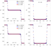 |
Fig. 1. Current sheet test (Komissarov 2004; Yu 2011) as described by the initial data in Eq. (72) on a x ∈ [−2,2] grid (fCFL = 0.25) at t = 1.0 for B0 = 0.5 and different resolutions. Two fast waves emerge from the original discontinuity and propagate outward with the speed of light (analytical position of the waves are indicated by dashed vertical lines). The order of convergence, 𝒪 is indicated according to Eq. (71). Top: MP7 reconstruction. Bottom: MC reconstruction. |
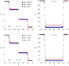 |
Fig. 2. Degenerate current sheet test (Komissarov 2004; Yu 2011) as as described by the initial data (Eq. (72)) with B0 = 2.0. Two fast waves emerge from the original discontinuity and propagate outward with the speed of light. The cross field conductivity (induced by conserving conditions (37), and (38)) terminates the fast waves in the breakdown-zone. Top: MP7 reconstruction. Bottom: MC reconstruction. |
If B0 < 1, there exists a force-free solution given by two fast waves traveling at the speed of light (see Fig. 1, also Fig. C2 in Komissarov 2004). For B0 > 1 the solution is dominated by an increasing cross-field conductivity that locks B2 − D2 to zero in a current sheet located at x = 0. At this location, the preservation of the force-free conditions (Sect. 3.3) becomes important for the field dynamics, namely it changes the structure of the propagating waves. The states bounded by the fast waves are terminated at the current sheet and a standing field reversal remains (see Fig. 2, cf. Fig. C2 in Komissarov 2004). We take advantage of this test to compare the performance of two different reconstruction schemes: The second-order accurate, slope limited TVD reconstruction with a monotonized central (MC) limiter (van Leer 1977), and the seventh-order accurate monotonicity preserving (MP7, Suresh & Huynh 1997) reconstruction.
From the results of the presented tests (Figs. 1 and 2), we draw the following conclusions. Fast electromagnetic waves propagate correctly at the speed of light. For a resolution similar to the one employed in Komissarov (2004), where Δx = 0.015, the time evolution of the (degenerate) current sheet is in good qualitative agreement with the literature (Komissarov 2004; Yu 2011). For resolutions below the lowest presented resolution (i.e., for Δx > 0.05) the wave structure of the presented test quickly smears out.
Conservation of force-free conditions in the degenerate current sheet test is working well and agrees with similar tests throughout the literature (see Fig. 3). While monotonicity preserving reconstruction is slightly more oscillatory than, for example, monotonized central flux limiters, the higher-order schemes allow a steeper resolution of wave-fronts and current sheets. While the order of convergence of the (more diffusive) MC reconstruction approaches the formal theoretical order of convergence (𝒪 = 2), the order of convergence degrades below its theoretical value for MP7.
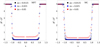 |
Fig. 3. Same scenario as Fig. 2. The panels show the magnetic dominance state (cf. Fig. C2, Komissarov 2004). D2 > B2 develops at the location of the central current sheet, such that the electric field is altered by the algebraic adjustment maintaining condition (38). Our numerical implementation of the adjustment (63) drives D2 − B2 → 0 instantaneously, restoring magnetic dominance. |
Although some degradation of the order of convergence is expected in non-smooth regions of the flow (e.g., the discontinuities associated with fast or Alfvén waves), the algebraic enforcement of the violated force-free conditions seems to have a large impact on the computed value of 𝒪. Very likely, such algebraic enforcement is the main source of deviation from the theoretical expectations regarding the order of convergence.
Given the previous statements, the developed GRFFE code passes the 1D (degenerate) current sheet test.
4.1.2. Three-wave and stationary alfvén wave test
Komissarov (2002), Yu (2011) and Paschalidis & Shapiro (2013) suggest the three-wave problem (or a variant thereof, see Fig. 4) as a test for force-free electrodynamics. The initial discontinuity at x = 0 splits into two fast discontinuities and one stationary Alfvén wave. This effectively combines the previously introduced test of Sect. 4.1.1 with the standing Alfvén wave test thats was also employed by Komissarov (2004). The initial electromagnetic field is given by (Paschalidis & Shapiro 2013):
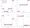 |
Fig. 4. Three-wave problem (Paschalidis & Shapiro 2013) as described by the setup in Eq. (73) and employing MP7 reconstruction. Numerical setup and labels are the same as in Fig. 1. The initial discontinuity at x = 0 splits into two fast discontinuities and one stationary Alfvén wave. |
We evolve this setup in time and present the results for different resolutions in Figs. 4 and 5. Around the standing Alfvén wave at x = 0, high-order reconstructions tend to develop small-scale oscillations, especially visible in the plots of Dx, restricted to the region delimited by the fast waves (at x = ±1 for t = 1). Oscillations around this discontinuity can also be observed (for higher resolutions) in part of the literature (specifically, Fig. 4 in Yu 2011). The order of convergence is slightly reduced when compared to the results shown in the previous section, probably due to the specific challenges of resolving stationary Alfvén waves, not only in GRFFE but also in relativistic MHD (see, e.g., Antón et al. 2010).
The empirical order of convergence grows employing MP7 in combination with a sixth-order accurate discretization of the parallel current (66). This growth manifests, for example, in an increase from 𝒪 ≈ 2.1 to 𝒪 ≈ 2.8 for Dx, but is negligible in other variables. In any case, the overall numerical solution does not significantly change modifying the order of accuracy of the calculation of j|| in the 1D problems involving discontinuities.
Komissarov (2004) achieves high accuracy maintaining a single standing Alfvén wave stationary during evolution for resolutions comparable to the highest one shown in Figs. 4 and 5. The numerical techniques in Komissarov (2004) are slightly different from ours, employing, for example, a linear Riemann solver, which makes use of the full spectral decomposition of the FFE equations. As such, it distinguishes all physical, and nonphysical wave speeds and may provide additional accuracy at critical locations (in the context of GRFFE, e.g., at current sheets). Additionally, Komissarov (2004) employs a different form of the current in Faraday’s Eq. (10) based on a specific (numerical) resistivity model to drive electromagnetic fields toward a force-free state throughout the evolution. Although one could suspect that this different treatment of the currents may alter the numerical solution significantly in this test (which is dominated by the numerical diffusivity of the standing wave), we find that our results are quite similar to the ones of Komissarov (2004); a more detailed analysis is presented in Paper II.
Next, we consider the analytical solution of a standing Alfvén wave as initial data in the following:
![$$ \begin{aligned}&\mathbf B =\left(1,1,B^z\right),\quad \mathbf D =\left(-B^z,0,1\right),\nonumber \\&B^z=\left\{ \begin{array}{cc} 1&x\le 0\\ 1+0.15\left[1+\sin \left[5\pi \left(x-0.1\right)\right]\right]&0 < x\le 0.2\\ 1.3&x>0.2 \end{array}\right. . \end{aligned} $$](/articles/aa/full_html/2021/03/aa38907-20/aa38907-20-eq99.gif)
We present the results of the Alfvén stationarity test in Fig. 6. With resolutions comparable to the one employed in Komissarov (2004), namely Δx ≈ 0.015, the numerical solution converges to the analytic one with an order of convergence of ≈2 for MP7 reconstruction. This order of convergence is dominated by the numerical errors around the transition layer 0 ≲ x ≲ 0.2. As mentioned in the previous tests, standing Alfvén waves seem to introduce severe degradation of the order of convergence in MP methods (we also verified these results with MP5). This is very likely related to the preservation of the D ⋅ B = 0 condition, in the extended region 0 ≤ x ≤ 0.2 where Bz is not uniform. In that region, the cutback of the electric displacement generates numerical errors that accumulate mostly close to its lower boundary (see the behavior of Dx in −0.5 ≲ x ≲ 0 in Fig. 5).
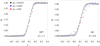 |
Fig. 6. Stationary Alfvén wave problem (Komissarov 2004), same numerical setup as in Fig. 1. The analytic solution (Eq. 74) is indicated by a gray line. |
4.2. FFE wave interaction (2D/3D)
We perform a test (explored in extensive detail and high resolution by Li et al. 2019) of the interaction between colliding Alfvén modes in suitably chosen 2D and 3D computational boxes. In this section, we intend to reproduce the most basic results of energy cascades from Alfvén wave interactions to show our GRFFE scheme’s ability to explore such phenomena in further detail in the future.
On the respective numerical meshes, one initializes counter-propagating Gaussian 2D or 3D wave packets traveling along a uniform guide field By = B0. Periodic boundary conditions facilitate the recurring superpositions and interaction of the wave packets, eventually triggering an energy cascade of rapid dissipation. The 3D Gaussian wave packets are initialized as

where  is the unit vector in the y-direction and the scalar field
In this section, ξ denotes the perturbation strength, l the width of the wave packet, with centers are located at r1 and r2. We follow Li et al. (2019) in choosing ξ = 0.5, l = 0.1, r1 = (0.5,0.25,0.5) and r2 = (0.5,0.75,0.5) for the 3D wave packets. With this setup, the field perturbation is purely azimuthal with respect to the y-axis. On a reduced 2D mesh, we initialize Gaussian wave packets with magnetic fields
where  is the unit vector in the z-direction and
We employ ξ = 0.4, l = 0.1, r1 = (0.5,0.25) and r2 = (0.5,0.75) for the 2D setup. The motion of the wave packets is induced with a drift speed D × B/B2, that results form an initial electric field

with opposite signs for each Gaussian wave packet.
After the initialization of the electromagnetic fields, the bounding box of length L = 1 and periodic boundaries are left to evolve for 200τ (fCFL = 0.2). τ = 0.5 is the interval between two subsequent collisions of the wave packets, and t/τ the number of collisions. For these tests, we employ MP7 reconstruction (with a fourth-order discretization of j∥). Following Li et al. (2019), we employ the free-energy U as the measure of total electromagnetic energy of the system etot under removal of the background magnetic field B0:
Figure 7 shows the free-energy for the collision of the wave packets defined in Eqs. (76) and (78). The wave packets are spherical and – due to their curvature – prone to redistribute energy across wave modes and rapid dissipation in cascade-like processes (e.g., Howes & Nielson 2013; Nielson et al. 2013). Such processes are likely to be found along curved guide-fields, for example in magnetar magnetospheres. Collisions excite waves of higher frequency than initially setup and eventually trigger the rapid decay of the wave free-energy. In order to make a more quantitative comparison of the results, we also compute the spectral distribution of free-energy according to components of the propagation wave vector which are parallel (k||) and perpendicular (k⊥) to the guide field, following the same prescription as in Li et al. (2019) (see Figs. 9 and 8). We compare our 2D and 3D results with the reference work of Li et al. (2019) below.
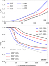 |
Fig. 7. Free-energy U (normalized to its initial value U0) during the collision of Alfvén wave packets on numerical meshes (2D/3D) of various resolutions (indicated by different line styles). Top: evolution of U0/U for the set of 2D models. Slopes for the asymptotic linear relation between U0/U and ln t are indicated by dashed/dotted lines, comparing to Fig. 7 of Li et al. (2019). Bottom: free-energy evolution normalized to U0 comparing to Figs. 2 and 5 from Li et al. (2019). The asymptotic slope for 3D models found by Li et al. (2019) is indicated by a gray dashed line for reference. |
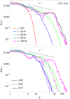 |
Fig. 8. Spectrum evolution for the 2D simulation of Alfvén interactions initialized according to Eq. (78). We show the spectral energy distribution for wavenumbers k⊥ (perpendicular to the guide field) in analogy to Fig. 6, Li et al. (2019). Top: spectral energy distribution at different times for the resolution 5122. Bottom: spectral energy distribution for selected times and wavenumbers (color code as in top panel) and different resolutions, indicated by dashed (1282), dotted (2562) and solid (5122) lines. No visible convergence is reached. |
4.2.1. 2D models
Our GRFFE code is able to reproduce the dissipation patterns of free electromagnetic energy presented in Fig. 5 of Li et al. (2019) for the 2D setup of Eq. (78). We note that our tests correspond to the lowest three mesh resolutions employed by Li et al. (2019). In the top panel of Fig. 7, we display the evolution of the inverted free-energy (U0/U) along with the slopes for their decay in 2D. Contrasting the findings by Li et al. (2019), the decay of U initially proceeds at the same rate (s ≈ 0.35) for all of the analyzed 2D models, independent of the chosen resolution. Only at later times, the slopes deviate and (roughly) approach the numerical values given in Fig. 7 of Li et al. (2019). The redistribution of spectral energy happens at all times from the smaller to the larger values of k⊥ (Fig. 8), and an approximate  spectral dependence is observed for intermediate values 10 ≲ k⊥ ≲ 70. The maximum value of k⊥, k⊥, max, is resolution dependent (the finer the resolution, the larger k⊥, max). Hence, there is no evidence of spectral convergence in 2D (in agreement with Li et al. 2019, see Fig. 8 lower panel). For the respective resolution, the decay of U begins later than in Li et al. (2019), suggesting that the numerical diffusivity in our method (combining MP7 reconstruction, a fourth-order accurate Runge-Kutta time-integrator and no additional driving terms in j||) is smaller (compared to a fifth-order spatial WENO reconstruction, a third order accurate Runge-Kutta time-integrator, and an extra dissipation term in j||). As a result, our models with a grid of 5122 zones display an evolution of U trending roughly in between the curves corresponding to ∼10242 and 20482 in Li et al. (2019). A more thorough characterization of the (numerical) dissipation of our algorithm is considered in Paper II.
4.2.2. 3D models
For tests in 3D, we are limited to the two lower resolutions of the corresponding model in Li et al. (2019) to stay within the computational costs that are reasonable for a test setup. In spite of the reduced resolution we employ compared to the literature, we find a remarkable agreement with the reference results. For instance, we observe a faster onset of the energy cascade than in 2D, and the same asymptotic value of the free-energy (U/U0 ≈ 0.4 for the best resolved 3D model; Fig. 7 lower panel; cf. with Fig. 2 of Li et al. 2019). We also find comparable (although slightly shallower) asymptotic slopes for the free-energy decay; the slope found by Li et al. (2019) is indicated in Fig. 7 with a dashed gray line. Another important key feature obtained by Li et al. (2019) is the existence of a characteristic time, tonset after which dissipation commences in 3D models. After this time there is a relatively sharp drop of the free-energy, which tends to level off for sufficiently long times. However, the feature that unanimously sets tonset (according to the definition of Li et al. 2019) is found in the evolution of the spectral energy distribution. Before tonset, the colliding Gaussian packets shuffle energy toward smaller scales (larger values of the wave number k) until a maximum k = kmax is reached. However, after t = tonset there exists a redistribution of energy from the smaller to the larger scales, which manifest itself as an increasing spectral power at small values of k. For Li et al. (2019), tonset ≈ 24τ. The conclusions of Li et al. (2019) are based upon 3D models with finer resolution than the ones employed in this section (e.g., models with 5123 and 7683 zones). With a smaller resolution, we also find a time after which there is a steep drop of the free-energy, which begins at t ≳ 30τ (Fig. 9 top panel). Nevertheless, we do not clearly see an increase in the spectral power at small values of k⊥, but we observe a decrease of power for k⊥ ≳ 30 for a time 30τ ≲ tonset ≲ 40τ. At about this time, the fast drop off in U takes place. Since we have evolved our models longer in time, we note that at t = 160τ there is a decrease of spectral energy at intermediate values 10 ≲ k⊥ ≲ 25 (Fig. 9 top panel). The spectral evolution of the modes parallel to the guide field proceeds qualitatively as in Li et al. (2019), with the only difference that we observe some (small) excess of power in the range 10 ≲ k|| ≲ 50. As in 2D, most of the (small) quantitative differences observed in the comparison with Li et al. (2019) results can be attributed to the different order of accuracy of our codes and the different terms entering in the current parallel to the magnetic field.
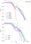 |
Fig. 9. Spectrum evolution for the 3D simulation of Alfvén interactions initialized according to Eq. (75). We show the spectral energy distribution for wavenumbers k⊥ (perpendicular to the guide field) in analogy to Fig. 2, Li et al. (2019). Top: spectral energy distribution at different times for the resolution 3843. Bottom: spectral energy distribution for selected times and wavenumbers (color code as in top panel) and different resolutions, indicated by dashed (1283), dotted (2563) and solid (3843) lines. For wavenumbers k⊥ ≲ 40, convergence is reached for the shown high-resolution cases. |
5. Astrophysically motivated tests
5.1. Magnetar magnetospheres
5.1.1. Grid aligned magnetar magnetospheres
The magnetospheres of magnetars are a well suited laboratory for numerical methods dealing with force-free plasma, and we have explored their dynamics in Mahlmann et al. (2019). Prior to those numerical simulations of a potentially very dynamic scenario, we performed numerical tests to assess the ability of our GRFFE code to maintain the structural stability of a magnetosphere around a spherical, nonrotating neutron star with a dipolar magnetic field. We use a spherical mask to cut out the neutron star interior in order to avoid dealing with the equation of state of nuclear matter, the different phases of matter that may occur inside of the neutron star, and the solid structure of the stellar crust. This is achieved by setting an internal boundary in a 3D Cartesian grid (i.e., stair-stepping along the spherical boundary mask) inside of which the evolution is frozen (see below). We note that 3D Cartesian coordinates are neither adapted to the spherical shape of the neutron star nor the axial symmetry of the magnetospheric dipole. Therefore, we expect significantly improved results when employing GRFFE in a spherical coordinate system. We compare the results of simulations in 3D Cartesian coordinates to axisymmetric (2D) tests in spherical coordinates, with the magnetic axis aligned to the symmetry axis of the initial data.
It is straightforward to specify the employed initial data in spherical coordinates (r,θ,ϕ) and, subsequently, map it to the computational grid. The analytically derived equilibrium dipolar magnetic field in (the coordinate basis of) spherical coordinates reads:
The Cartesian simulations are conducted in a 3D box with dimensions [4741.12 M⊙×4741.12 M⊙×4741.12 M⊙] with a grid spacing of Δx, y, z = 74.08 M⊙ on the coarsest grid level. For the chosen magnetar model of radius R* = 9.26 M⊙, this corresponds to a [512R*×512R*×512R*] box with a grid spacing of Δx, y, z = 8R*. For the low-resolution and high-resolution tests, we employed seven and eight additional levels of mesh refinement, respectively, each of which increase the resolution by a factor of two and encompass the central object. This means that the finest resolution of our models (close to the magnetar surface) are  and
and  for the low and high-resolution models. This corresponds to 16 and 32 points per R*, respectively. The spherical simulations are conducted in axial symmetry enclosing the volume [9.26 M⊙,2555.76 M⊙−6Δr] × [0,π]. In order to issue a resolution that is comparable to the Cartesian setup, we employ Δr ∈ [R*/16,R*/32] and Δθ ∈ [π/50,π/100]. The setup is evolved for a period of t = 1185.28 M⊙ ≃ 5.84 ms. We provide extensive details on the internal boundary conditions (frozen electromagnetic fields but balanced radial current) in Mahlmann et al. (2019). For this section we employ fCFL = 0.2, the MP7 reconstruction and a fourth-order accurate discretization of j||. We note that in this test we assume a flat spacetime. More general tests including a general relativistic, dynamically evolving background have been considered, for example, in Ruiz et al. (2014). However, performing such tests here is beyond the scope of this paper.
The stability test initializes the dipole structure throughout the entire computational domain and tracks the stability during a dynamical evolution. The relaxation test is even more challenging than the stability test since it requires the time evolution toward the physical topology set by the boundary conditions. Precisely, in a relaxation test we fix the dipolar structure inside of the star, but fill the magnetosphere with a purely radial field at the start of the simulation. In order to track the changes in the magnetosphere, we define its total energy as the volume integral
Once initialized, the energy of the dipole magnetosphere (cf. Mahlmann et al. 2019) is well conserved (stability) or else gradually approaches the dipole energy (relaxation) once all initially introduced perturbations leave the domain. Figure 10 shows stability and relaxation tests of the dipole magnetosphere for different resolutions in both, Cartesian (3D) and spherical (2D, axial symmetry) coordinates.
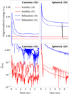 |
Fig. 10. Stability and relaxation test of magnetar magnetospheres endowed with an analytic dipole field structure for different resolutions. Upper panels: total magnetospheric energy normalized to the energy of the corresponding dipole. Lower panels: time derivative of the energy normalized to the dipole. The resolutions of 16 and 32 points per stellar radius in a 3D Cartesian CARPET grid (left) correspond to the setup in Mahlmann et al. (2019). Axially symmetric simulations in spherical coordinates (right) are set up with the indicated resolution at the stellar surface. Black (solid and dashed) lines in the upper-right panel correspond to a simulation on a smaller domain, extending up to r = 935.26 M⊙ − 6Δr, in which the pulses of the initial relaxation have sufficient time to leave the domain. |
The initial spike of the relaxation model can be attributed to a surge of electromagnetic energy during a rapid rearrangement in the early phase. The excited energy pulses propagate as plasma waves through the magnetosphere. A part of these pulses is confined to closed field lines in the vicinity of the central object. The rest of this energy propagates outward through the domain. As the dissipation of electromagnetic energy in collisions of force-free waves strongly depends on the employed resolution (see Sect. 4.2, and Paper II) and grid geometry, the confined energy pulses remain within the domain longer for higher resolution and spherical coordinates. This is visible best in the relaxation test presented in Fig. 10. For different resolutions, the asymptotic energy differs by < 1%. Complete relaxation of this energy will require longer simulation times, such that waves emerging from the initial relaxation can leave the domain. Also, accurate treatment of the interior boundary will be necessary so that plasma waves in the region of closed field lines dissipate physically. The first of these effects, associated with the total simulated time, can be partly addressed by considering a computational domain with a reduced outer radial boundary. In the top right panel of Fig. 10, we show the time evolution in a reduced computational domain with black lines. The abrupt drop-off the magnetospheric energy is due to the desertion of the initial perturbation through the outer radial boundary. Remarkably, the energy level to which these models evolve is the same as the corresponding stability tests with the corresponding numerical resolution.
5.1.2. Tilted magnetar magnetospheres
In this section, we explore the full 3D capabilities of our newly developed code in spherical coordinates (r,θ,ϕ) by considering the stability test from the previous section, but tilting the magnetic dipole axis by an angle α with respect to the spherical polar axis along θ = 0. For this, we carry out the transformation  , where
  , B corresponds to the initial data given in Eq. (81), and
![$$ \begin{aligned} \mathbf R _{-\alpha }&=\left[\begin{array}{ccc} 1&0&0\\ 0&\frac{\cos \alpha \sin \theta -\sin \alpha \cos \theta \sin \phi }{\chi }&\sin \alpha \cos \phi \\ 0&-\frac{\sin \alpha \csc \theta \cos \phi }{\chi }&\cos \alpha -\sin \alpha \cot \theta \sin \phi \\ \end{array}\right],\nonumber \\ \chi&=\sqrt{\sin ^2\theta \cos ^2\phi +\left(\sin \alpha \cos \theta -\cos \alpha \sin \theta \sin \phi \right)^2}. \end{aligned} $$](/articles/aa/full_html/2021/03/aa38907-20/aa38907-20-eq115.gif)
We chose α = 30° for simulations that are exclusively conducted in a spherical domain with dimensions [9.26 M⊙,611.16 M⊙−6Δr] × [0,π] × [0,2π]. In order to use a resolution that is comparable to Sect. 5.1.1, we employ Δr ∈ [R*/16, R*/24, R*/32] and Δϕ = Δθ ∈ [π/50, π/75, π/100]. The setup was evolved for a period of t = 300 M⊙ ≃ 1.48 ms with fCFL = 0.25 using MP7 spatial reconstruction and the default fourth-order discretization of j||.
Besides the measurement of the total energy in the magnetosphere, in order to quantify the deviation of the numerical solution B from the analytical (initial) configuration B0, we define the l2 error norm of the magnetic field as
![$$ \begin{aligned} ||\epsilon ||_2=\frac{1}{N}\sqrt{\sum _{i,\,j,\,k}\left[\mathbf B (r_i,\theta _j,\phi _k)-\mathbf B _0(r_i,\theta _j,\phi _k)\right]^2}, \end{aligned} $$](/articles/aa/full_html/2021/03/aa38907-20/aa38907-20-eq116.gif)
where indices i, j, and k extend over all the computational cells. Figure 11 shows the evolution in time of the error norm in Eq. (84) normalized to the magnetic field strength at the pole of the neutron star, Bp. Increasing the mesh resolution by a factor of two (i.e., from Δr = R*/16 to R*/32) reduces the error by roughly the same factor. At the same time, the total magnetospheric energy slightly increases throughout the simulation time (≲1%). Such a (continuous) increase in energy does not occur in the aligned (axially symmetric) setups, as we show in Fig. 10. However, the global structure of the 3D tilted dipole is conserved throughout the simulation (Fig. 11), with only slight kinks arising around the polar axis of the spherical coordinates.
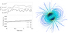 |
Fig. 11. Stability test of magnetar magnetospheres endowed with a tilted (30 degrees) analytic dipole field structure for different resolutions. Left: evolution of the l2-norm of the error with respect to the analytical (initial) configuration normalized to the magnetic field strength Bp at the magnetar pole (top), and of the total magnetospheric energy content (bottom). Right: 3D impression of the final state (t ≈ 1.5 ms) of the intermediate resolution simulation (Δr = R*/24). We display the magnetic field lines colorized by their norm. |
Solving hyperbolic PDEs in spherical coordinates suffer from very small timesteps due to the fact that cell volumes are not constant in space and get smaller as the polar axis or the origin of the coordinate system are approached. The timestep is proportional to r × sin(Δθ/2) × Δϕ and hence becomes prohibitively small for full 3D simulations with high angular resolutions, this is the reason for the shorter simulation time compared to the axially symmetric models in Sect. 5.1.1). In order to mitigate this limitation for simulations in spherical coordinates, additional grid coarsening or filtering approaches will be necessary when considering computationally feasible long-term 3D evolution (cf. Obergaulinger & Aloy 2017, 2020; Mewes et al. 2020; Zlochower et al., in prep.; Aloy & Obergaulinger 2021). The impact of the tilt across the axis on the magnetospheric energy (as observed in Fig. 11) may be further diminished by such techniques.
In this test we employ the full 3D capacities of our GRFFE method in spherical coordinates. The tilted magnetar magnetospheres maintain their topology stable for ∼32 light-crossing times of the central object. Extrapolating the deviation of the magnetospheric energy to longer times is uncertain due to the non-monotonic evolution. However, we foresee that stationary tilted magnetospheres may be maintained approximately stable sufficiently for more than a few hundred light-crossing times of the central object. These longer periods of evolution may suffice to address numerically dynamical phenomenae in the magnetosphere (e.g. Carrasco et al. 2019; Mahlmann et al. 2019). Besides, our results show that increasing the resolution decreases the global error, hence, if needed, finer grids may be used to address longer evolutionary times.
5.2. The force-free aligned Rotator
An astrophysically motivated test that deliberately breaches the limits of FFE is the aligned rotator test. It sets up an initially dipolar magnetic field on a star rotating with angular velocity Ωp. Equilibrium solutions of the axisymmetric pulsar magnetospheres, as solutions to the so-called pulsar equation, have been studied, for example, in Contopoulos et al. (1999) and Timokhin (2006). Time-dependent solutions to the aligned rotator magnetosphere have been presented; for instance, by Komissarov (2006, resistive MHD and resistive FFE), Spitkovsky (2006, resistive FFE), Paschalidis & Shapiro (2013, dissipative FFE), Tchekhovskoy et al. (2013, MHD), Etienne et al. (2017, dissipative FFE). All of these schemes make sure that the equatorial current sheet can be resolved in FFE by either adding additional dissipation or a resistivity model to FFE, or by combining FFE and MHD in order to capture such genuinely non-force-free regions.
In this section, we present results of the aligned rotator test in ideal FFE conducted on a spherical, axisymmetric mesh. We demonstrate that our code correctly reproduces the features of the force-free magnetosphere inside of the pulsar light cylinder rLC = c/Ωp. We transparently point out the consequences of the emerging equatorial current sheet in ideal FFE, to which we ultimately dedicate paper II of this series (Mahlmann et al. 2021). This test sets up the initial data of Eq. (81) in a domain with dimensions [9.26 M⊙,6954.26 M⊙−6Δr] × [0,π]. We employ Δr ∈ [R*/16, R*/32, R*/64] and Δϕ= Δθ ∈ [π/50, π/100, π/200]. The setup is evolved for a period of t = 3150 M⊙ (10 revolutions of the central object) with fCFL = 0.25, using MP5 spatial reconstruction, and the default fourth-order discretization of j||. We implement the pulsar boundary condition by following closely the interior boundary conditions described by Parfrey et al. (2012) and setting Ωp = 0.02.
Figure 12 visualizes the results of this resolution study. Our code correctly reproduces the expected magnetospheric features for r < rLC. A twist-free, closed region emerges for r ≲ 0.8rLC. There, field lines co-rotate with the central object in good accordance with the imposed pulsar boundary conditions. Slight deviations from perfect co-rotation (of a few percent, decreasing with higher resolution) occur at the sheath of the twist-free region. The location of the Y-point r ∼ 0.9rLC is stable for the employed resolution. As reasoned in Spitkovsky (2006), reconnection is the key factor setting the location of the Y-point, rY relative to rLC, as well as the rate at which rY approaches rLC from its initial location. The effects of a finite (numerical) resistivity induce an oscillatory behavior of the Y-point as well as (in the case of Spitkovsky 2006) the ejection of (small) plasmoids. Episodically, non-axisymmetric, small-scale structures emerge out of the equatorial current sheet. The scale and temporal wavelength of the variations in the current sheet decrease with increasing resolution (middle panels Fig. 12b). The unsteadiness of the current sheet is a direct consequence of the very low numerical resistivity of our high-order schemes applied to ideal FFE. They significantly reduce the numerically driven reconnection (cf. Mahlmann et al. 2021). The morphology of the current sheet results from localized (numerical) reconnection events that happen as a result of the enforcement of the magnetic dominance condition (B2 − E2 ≥ 0) at low latitudes, where the magnetic field strength passes through zero as it crosses the equator. In the absence of a more elaborated physical description of the layer where the plasma pressure becomes larger than the magnetic pressure (e.g., using MHD), recipes to handle the numerical resistivity completely determine the spatial smoothness and time variability of the equatorial current sheet.
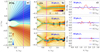 |
Fig. 12. Force-free aligned rotator test in spherical ideal FFE for different resolutions. Left panel a: global structure of the magnetosphere for intermediate resolution (32 pts./r*). The poloidal fieldlines are indicated by black solid and dashed lines, depending on the magnetic field direction. Blue and red colors represent direction and magnitude of the toroidal magnetic field (normalized to its maximum value). Middle panel b: zoom on the Y-point and equatorial current sheet (alternating magnetic field highlighted by cyan field lines) for different resolutions. The color scale represents the current density (normalized to the current density of the low-resolution data). Left panel c: field line angular velocity measured at different radii. |
The Poynting flux of outflowing energy agrees well with the expectations collected in the literature, L ≈ (1.0+0.1)L0 (for the highest-resolution run), where  for a magnetic moment μ. The value of L larger than L0 is directly related to the fact that rY < rLC during the computed time. On longer time-scales (computationally prohibitive for a single code test) the luminosity decreases as the closed zone expands (Spitkovsky 2006), something that generically happens for all resolutions considered here (but at significantly different rates; faster at lower resolution). For the lowest employed resolution (16 pts./r*), we find that the luminosity gradually decreases by ∼10% for r < 5rLC. For higher resolutions, the luminosity level is stable but showing variations due to small structures emerging in the current sheet (middle panels Fig. 12b). Our rigid confinement to only enforcing the FFE conditions (Sect. 3.3) without adding additional dissipation mechanisms or resistivity models is the main difference to the aforementioned array of literature available for this particular setup.
The results presented in this section are sensitive to both the boundary conditions and the modeling of the equatorial current sheet. As general features of the force-free magnetosphere (r < rLC) are reproduced as expected (twist-free region, field line angular velocity and luminosity), our code passes the ideal FFE aligned rotator test. We stress, however, that a physical modeling of the equatorial current sheet beyond the Y-point requires suitable techniques to develop such genuinely resistive regions in time. In Mahlmann et al. (2021), we outline the difficulties and some possible remedies of this task. We are convinced that a physical modeling of equilibrium solutions containing both force-free regions and current sheets either requires exceptional fine-tuning of the employed resistivity models, or a mixing of different plasma regimes (such as FFE and resistive MHD; see, e.g., Ruiz et al. 2014). In any case, such modeling is beyond the scope of a test for ideal FFE.
5.3. Black hole magnetospheres
5.3.1. Black hole monopole tests
Blandford & Znajek (1977) presented analytic equilibrium solutions of BH magnetospheres by applying perturbation techniques to the Grad-Shafranov equation (GSE) that match the Znajek condition (Znajek 1977) at the BH horizon and the flat space solution of Michel (1973) at infinity. One of these results is a monopole-like magnetic field, which is often adapted to the so-called split monopole by mirroring the field quantities across the equatorial plane. The latter is a necessary step to avoid divergences of the magnetic field. In this section, however, we follow Komissarov (2004) in considering the monopole field structure to avoid the challenge of resolving a current sheet at the equator. The monopole electromagnetic fields for slowly spinning BHs (a* ≪ 1) as derived in Blandford & Znajek (1977) can be written in the spatial components of vectors in Boyer-Lindquist coordinates (r,θ,ϕ) as follows:

Here, ΩF is the field line angular velocity as defined for axially symmetric equilibrium solutions, and we employ B0 = 1. The Cartesian simulations are conducted in a 3D domain with extensions [256 M⊙×256 M⊙×256 M⊙] with a grid spacing of Δx, y, z = 8 M⊙ on the coarsest grid level. We use eight additional levels of mesh refinement, each increasing the resolution by a factor of two and encompassing the central object, respectively. This means that the finest resolution of our Cartesian models is  . The spherical simulations are conducted on a 2D slab (axial symmetry) with extensions [0,256 M⊙] × [0,π]. In order to use a resolution that is comparable to the Cartesian setup, we employ Δr = 0.032 and Δθ = π/64. The setup is evolved for a period of t = 128 M⊙. For this section we employ fCFL = 0.25, the MP7 reconstruction and a fourth-order accurate discretization of j||.
Figure 13 summarizes the time evolution of the monopole field for a dynamically evolving spacetime metric for both Cartesian (3D) and spherical (2D, axisymmetric) meshes. As the magnetospheres considered in this section (and the following one) are idealized cases, namely a magnetic monopole and with unbound energy, we do not couple the field energy to the source terms of the BSSN equations. During a transient phase in which the metric terms relax to the chosen mesh and gauge, the electromagnetic fields can differ significantly from their initial state. This test demonstrates that, while the spacetime evolves, the electromagnetic fields relax toward the equilibrium given by Eq. (85) concurrently. Though the energy evolution shown in Fig. 13 approaches the energy of the initial model rather well, the resulting equilibrium has to be taken with care. The evolution of dynamical spacetimes and corresponding GRFFE fields can be subject to the influence of small changes of the BH mass and spin (due to finite numerical resolution), as well as an involved array of geometric source terms (see Sect. 2.2).
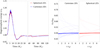 |
Fig. 13. Time evolution of the Schwarzschild monopole (ΩF = ΩBH/2) of a slowly spinning Kerr BH (a* = 0.1, M = 1) in Cartesian (3D CARPET grid with nine refinement levels, with the highest resolution of 0.03125 M⊙ completely enclosing the central object) and spherical (2D, axsymmetric) coordinates. The spacetime metric is dynamically evolving. Left: evolution of the total magnetospheric (electromagnetic) energy normalized to the initial value, e0. Right: field line angular velocity along the equatorial plane. The final value is shown in a strong color. Intermediate states throughout the simulation are depicted by lighter colored lines (the strength of the color increasing with simulation time). |
The geometric (i.e., spacetime) quantities determined by the initial data for spinning BHs presented in Liu et al. (2009) relax to their equilibrium state depending on the chosen numerical resolution of the mesh and specification of gauge quantities (i.e., the lapse and shift) during an initialization phase. The choice of these quantities is preferably done in a way that causes the least possible noise across all metric quantities during their evolution. As an example, instead of providing the spacetime data with the analytic lapse function defined in Boyer-Lindquist coordinates (Liu et al. 2019), we specify the lapse initially as:
![$$ \begin{aligned} \tilde{\alpha }(0)=2\times \left[1+\left(1+\frac{M}{2r}\right)^4\right]^{-1}. \end{aligned} $$](/articles/aa/full_html/2021/03/aa38907-20/aa38907-20-eq120.gif)
With this initialization, the spacetime relaxes swiftly to its equilibrium state during the first Δtinit ≈ 25 M⊙. The tests presented in this section give some important hints on the strategies chosen to set up BH magnetospheres for our future research. The goal of this test was to show that the magnetospheric data are conserved throughout the (dynamic) relaxation of the spacetime induced, for example, by the BSSN algorithms of the EINSTEIN TOOLKIT. As both the magnetospheric energy as well as the field line angular velocity at the equator, are recovered after Δtinit, our GRFFE code passes this test of spacetime-field coupling.
5.3.2. The Wald magnetosphere
The immersion of a BH into a magnetic field that is uniform at infinity was originally suggested by Wald (1974) and then explored throughout the literature, both as a test and as a laboratory for force-free plasma (Komissarov 2004; Komissarov & McKinney 2007; Carrasco & Reula 2017; Parfrey et al. 2019). In this section, we reproduce the initial data of the Wald magnetosphere of a Schwarzschild BH in Boyer-Lindquist coordinates (rescaled according to the prescription of Liu et al. 2009) and evolve it for different BH spins. We therefore, extend the testing of the GR capacities of our code to rapidly spinning BH (up to a* = 0.9). The Wald magnetosphere of a Schwarzschild BH in the spatial components of Boyer-Lindquist coordinates (r,θ,ϕ) can be initialized as follows:
We employ B0 = 1 as normalization of the magnetic field strength. The Cartesian simulations are conducted in a 3D domain with extensions [512 M⊙×512 M⊙×512 M⊙] with a grid spacing of Δx, y, z = 16 M⊙ on the coarsest grid level. We employ nine additional levels of mesh refinement, such that the finest resolution of our Cartesian models is  . The spherical simulations are conducted in axial symmetry with extensions [0,256 M⊙] × [0,π]. In order to use a resolution which is comparable to the Cartesian setup, we employ Δr = 0.032 and Δθ = π/64. The setup is evolved for a period of t = 128 M⊙ in Cartesian coordinates and t = 256 M⊙ in spherical coordinates. For this section we employ fCFL = 0.25, the MP7 reconstruction and a fourth-order accurate discretization of j||.
Figure 14 shows the results from the time evolution of these fields in spacetimes of rotating BHs for a selected case (a* = 0.5) in Cartesian and spherical coordinates. The magnetic field lines connecting to the BH, which are initially not rotating, are gradually twisted in case of a spinning central object. Also, current sheets form along the equatorial plane within the BH ergosphere for high dimensionless spins (a* = 0.9, Fig. 15), preventing the development of static magnetospheric conditions (cf. Komissarov 2004). The overall topology of the magnetic field throughout the BH ergosphere broadly coincides with respective equilibrium solutions of Kerr magnetospheres (as derived, e.g., in Nathanail & Contopoulos 2014; Mahlmann et al. 2018).
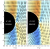 |
Fig. 14. Simulations of Wald magnetospheres for a* = 0.5 and M = 1 at t = 128 M⊙. Left: 3D Cartesian CARPET grid (vacuum spacetime modeled by MACLACHLAN). Right: 2D (axially symmetric) spherical grid (vacuum spacetime modeled by SPHERICALBSSN). The poloidal field is indicated by streamlines, the toroidal field by red and blue colors (color scale coincides for all panels) indicating whether the toroidal field leaves or enters into the displayed plane, respectively. The BH ergosphere is denoted by a solid white line. |
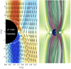 |
Fig. 15. Simulations of a Wald magnetosphere for a* = 0.9 in Cartesian coordinates for t = 256 M⊙. Left: same format and color scale as in Fig. 14. Right: 3D magnetic field line impression of the Wald magnetosphere. Darker colors indicate a stronger twist of the magnetic field. |
The simulations in spherical coordinates are significantly more expensive than in Cartesian coordinates, due to the severe restrictions on the timestep imposed by the converging spherical mesh close to the central singularity. Future code developments will include mesh-coarsening strategies close to r = 0 to overcome this restriction. Alternatively, we may use other methods to exclude the BH singularity from our computational domain (e.g., using shifted Kerr-Schild coordinates as in Paschalidis & Shapiro 2013). Obtaining a stable evolution of the spacetime with spherical coordinates for a* ≳ 0.9 is very challenging unless we employ rather fine grid spacing in θ, which makes this numerical experiment (currently) too expensive as a validation test of our code. Even in axisymmetric simulations, the timestep restriction from the θ coordinate, which imposes a timestep proportional to r × Δθ, is too restrictive when the coordinate origin is included in the computational domain, which is necessary for a spacetime evolution without excision as the one employed here. In order to alleviate this shortcoming of doing high-resolution simulations in spherical coordinates that include the origin, algorithms to circumvent the timestep restrictions imposed by both the θ and ϕ coordinates are currently being developed (Zlochower et al., in prep.).
In Fig. 16 we extract the field line angular velocity and toroidal magnetic field at different locations for Cartesian coordinates for comparison with Fig. 5 in Komissarov (2004) (computed for a BH with a* = 0.9). The chosen extraction location is slightly different from the literature in order to represent the complete range of BH spins. We find that our GRFFE code qualitatively reproduces the results in the literature, though some differences remain to be mentioned. Komissarov (2004) uses spherical coordinates and axial symmetry, as opposed to our 3D simulations with mesh refinement. More even, the angular resolution of 800 cells in the θ-direction is almost ten times the resolution that we used on our finest refinement level (the resolution limit is simply imposed by the aim of running numerical tests that do not consume disproportionate computational resources). Without evolving the spacetime (as in Komissarov 2004) the numerical grid may extend outward in the radial direction from the event horizon as a boundary, in practice, excising the central singularity and allowing for significantly larger timesteps. A similar effect may have the usage of shifted Kerr-Schild coordinates (as in Paschalidis & Shapiro 2013). The quantitative difference in the shape of the angular velocity distribution (V-shape in Fig. 5 of Komissarov 2004, vs. U-shape in Fig. 16) may, hence, be significantly improved with increasing resolution or by resorting to a GRFFE code in spherical coordinates (as we plan to do once the timestep restrictions are overcome). Also, we point out that we show the toroidal component of the magnetic field B rather than H. The overall form of the toroidal field for the rapidly rotating case (a* = 0.9) corresponds well (up to a difference in sign) with Fig. 5 of Komissarov (2004). The BH magnetosphere simulations in this section have been repeated on a fixed Kerr-Schild background metric, effectively confirming the results presented in this section. For a direct comparison of numerical data, comparable resolutions and exact convergence (longer simulations) are required; this is beyond the scope of the test presented here.
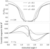 |
Fig. 16. One-dimensional values of the field line angular velocity (top) and the toroidal magnetic field (bottom) for the Wald test (Cartesian CARPET grid) at t = 256 M⊙ and using different BH dimensionless rapidities (see legends). The interpolation radius (for the extraction in a Cartesian grid) is indicated in the respective panel, corresponding to the ergosphere radius at the equator (top) or the BH horizon radius (bottom). |
We finally note that the small numerical resistivity of our code (prompted by the spatial high-order of our MP reconstruction methods; see Paper II) inhibits, in part, the formation of a stationary current-sheet in the solution. For that to happen, one needs to add extra dissipation at current sheets, for example by modifying Ohm’s law (as in, e.g., McKinney 2006) or artificially decreasing the conductivity perpendicular to field lines (Paschalidis & Shapiro 2013). The ideal FFE aligned rotator test presented in Sect. 5.2 lucidly illustrates this statement.
In conclusion, especially field lines threading the ergosphere are gradually twisted by the rotating BH. Due to the broad coincidence with Komissarov (2004), and the reproduction of magnetospheres which resemble respective equilibrium solutions of the (Nathanail & Contopoulos 2014; Mahlmann et al. 2018), the Wald magnetosphere test is passed.
6. Conclusions
We have developed a new GRFFE code that models magnetically dominated plasma in dynamical spacetimes with support for both Cartesian and spherical coodinates provided by the CARPET grid of the EINSTEIN TOOLKIT. Our simulation tool combines techniques from an array of literature (especially Komissarov 2002; McKinney & Gammie 2004; Palenzuela et al. 2009; Paschalidis & Shapiro 2013; Parfrey et al. 2017) and improves further on numerical strategies as well as the understanding of their limits:
-
We explicitly couple the continuity equation of charge to our conservative scheme (Sect. 2) and, thus, ensure a consistent modeling of the force-free current (Eq. (49)).
-
We employ a hyperbolic/parabolic cleaning of errors (extending the techniques in Palenzuela et al. 2009; Mignone & Tzeferacos 2010, to general relativity). Allowing for arbitrary advection speeds for the cleaning of divergence errors significantly improves the conservation of total charge in spacetimes of spinning BHs (see Appendix A).
-
The current parallel to the magnetic field j∥ is the dominant driver of resistivity in GRFFE schemes. In case of the force-free current (Eq. (64)), high-order discretization allows us to model (smooth) force-free plasma waves with nearly theoretical order (Sect. 2.1, Paper II), and diffusing only due to numerical resistivity.
-
Current sheets are genuine regions of significant physical resistivity. Conventional GRFFE methods (i.e., schemes that do not include phenomenological models of artificial physical resistivity) are unable to properly resolve such resistive layers, especially for highly accurate reconstruction methods (Paper II). Thus, at discontinuities, the order of convergence of GRFFE is significantly reduced; a true limit of applicability of GRFFE is reached.
Writing our EINSTEIN TOOLKIT thorn from scratch enabled us to implement suitable finite volume integrators for both Cartesian and spherical coordinates. Spherical coordinate systems prove exceptionally valuable for the highly accurate modeling of magnetar magnetospheres (Sect. 5.1). For the simulation of BH magnetospheres on dynamically evolving spacetimes, our GRFFE method will benefit from future updates to the support of spherical coordinates in the EINSTEIN TOOLKIT (Mewes et al. 2018, 2020). With the presented numerical code we broadly exploit the modular nature of the EINSTEIN TOOLKIT and implement a cutting-edge tool for the simulation of GRFFE on dynamical spacetimes in Cartesian and spherical coordinates.
Another evolution scheme, developing energy fluxes rather than electric fields, was employed by e.g., McKinney (2006) or Etienne et al. (2017).
Refluxing at mesh refinement interfaces by Erik Schnetter: https://svn.cct.lsu.edu/repos/numrel/LSUThorns/Refluxing/trunk
Acknowledgments
We appreciate the helpful comments and perspectives contributed by the anonymous referee. J. M. acknowledges a Ph.D. grant of the Studienstiftung des Deutschen Volkes. We acknowledge the support from the grants AYA2015-66899-C2-1-P, PGC2018-095984-B-I00, PROMETEO-II-2014-069, and PROMETEU/2019/071. We acknowledge the partial support of the PHAROS COST Action CA16214 and GWverse COST Action CA16104. P. C. D. acknowledges the Ramon y Cajal funding (RYC-2015-19074) supporting his research. V. M. is supported by the Exascale Computing Project (17-SC-20-SC), a collaborative effort of the U.S. Department of Energy (DOE) Office of Science and the National Nuclear Security Administration. Work at Oak Ridge National Laboratory is supported under contract DE-AC05-00OR22725 with the U.S. Department of Energy. V. M. also acknowledges partial support from the National Science Foundation (NSF) from Grant Nos. OAC-1550436, AST-1516150, PHY-1607520, PHY-1305730, PHY-1707946, and PHY-1726215 to Rochester Institute of Technology (RIT). The shown numerical simulations have been conducted on infrastructure of the Red Española de Supercomputación (AECT-2020-1-0014) as well as of the University of Valencia Tirant and LluisVives supercomputers.
References
- Alcubierre, M. 2008, Introduction to 3+1 Numerical Relativity (Oxford University Press) [Google Scholar]
- Alcubierre, M., Brügmann, B., Diener, P., et al. 2003, Phys. Rev. D, 67, 084023 [Google Scholar]
- Alic, D., Moesta, P., Rezzolla, L., Zanotti, O., & Jaramillo, J. L. 2012, ApJ, 754, 36 [Google Scholar]
- Aloy, M.-Á., & Obergaulinger, M. 2021, MNRAS, 500, 4365 [Google Scholar]
- Antón, L., Zanotti, O., Miralles, J. A., et al. 2006, ApJ, 637, 296 [Google Scholar]
- Antón, L., Miralles, J. A., Martí, J. M., et al. 2010, ApJS, 188, 1 [Google Scholar]
- Baumgarte, T. W., & Shapiro, S. L. 1999, Phys. Rev. D, 59, 024007 [Google Scholar]
- Baumgarte, T. W., & Shapiro, S. L. 2003, ApJ, 585, 921 [Google Scholar]
- Baumgarte, T. W., & Shapiro, S. L. 2010, Numerical Relativity: Solving Einstein’s Equations on the Computer (Cambridge University Press) [Google Scholar]
- Baumgarte, T. W., Montero, P. J., Cordero-Carrión, I., & Müller, E. 2013, Phys. Rev. D, 87, 044026 [Google Scholar]
- Beloborodov, A. M., & Thompson, C. 2007, ApJ, 657, 967 [Google Scholar]
- Beskin, V. S. 1997, Sov. Phys. Usp., 40, 659 [Google Scholar]
- Blandford, R. D., & Znajek, R. L. 1977, MNRAS, 179, 433 [Google Scholar]
- Bona, C., Masso,, J., Seidel, E., & Walker, P. 1998, ArXiv e-prints [arXiv:gr-qc/9804052] [Google Scholar]
- Brown, J. D. 2005, Phys. Rev. D, 71, 104011 [Google Scholar]
- Brown, J. D. 2009, Phys. Rev. D, 79, 104029 [Google Scholar]
- Brown, D., Diener, P., Sarbach, O., Schnetter, E., & Tiglio, M. 2009, Phys. Rev. D, 79, 044023 [Google Scholar]
- Carrasco, F. L., & Reula, O. A. 2016, Phys. Rev. D, 93, 085013 [Google Scholar]
- Carrasco, F. L., & Reula, O. A. 2017, Phys. Rev. D, 96, 063006 [Google Scholar]
- Carrasco, F., Viganò, D., Palenzuela, C., & Pons, J. A. 2019, MNRAS: Lett., 484, L124 [Google Scholar]
- Cerdá-Durán, P., Font, J. A., Antón, L., & Müller, E. 2008, A&A, 492, 937 [NASA ADS] [CrossRef] [EDP Sciences] [Google Scholar]
- Collins, D. C., Xu, H., Norman, M. L., Li, H., & Li, S. 2010, ApJS, 186, 308 [Google Scholar]
- Contopoulos, I., Kazanas, D., & Fendt, C. 1999, ApJ, 511, 351 [Google Scholar]
- Cordero-Carrión, I., Ibáñez, J. M., Gourgoulhon, E., Jaramillo, J. L., & Novak, J. 2008, Phys. Rev. D, 77, 084007 [Google Scholar]
- Darmois, G. 1927, Mémorial des Sciences Mathématiques, 25, 1 [Google Scholar]
- Dedner, A., Kemm, F., Kröner, D., et al. 2002, J. Comput. Phys., 175, 645 [Google Scholar]
- Diener, P., Dorband, E. N., Schnetter, E., & Tiglio, M. 2007, J. Sci. Comput., 32, 109 [Google Scholar]
- Dreyer, O., Krishnan, B., Shoemaker, D., & Schnetter, E. 2003, Phys. Rev. D, 67, 024018 [Google Scholar]
- Etienne, Z. B., Wan, M.-B., Babiuc, M. C., McWilliams, S. T., & Choudhary, A. 2017, CQG, 34, 215001 [Google Scholar]
- Event Horizon Telescope Collaboration (Akiyama, K., et al.) 2019a, ApJ, 875, L1 [NASA ADS] [CrossRef] [Google Scholar]
- Event Horizon Telescope Collaboration (Akiyama, K., et al.) 2019b, ApJ, 875, L5 [Google Scholar]
- Fourès-Bruhat, Y. 1952, Acta Math., 88, 141 [Google Scholar]
- Gammie, C. F., McKinney, J. C., & Tóth, G. 2003, ApJ, 589, 444 [Google Scholar]
- Goldreich, P., & Julian, W. H. 1969, ApJ, 157, 869 [Google Scholar]
- Goodale, T., Allen, G., Lanfermann, G., et al. 2003, in Vector and Parallel Processing - VECPAR’2002, 5th International Conference, (Springer), Lect. Notes Comput. Sci., 197 [Google Scholar]
- Gourgoulhon, E. 2012, 3+1 Formalism in General Relativity (Springer) [Google Scholar]
- Harten, A., Lax, P. D., & van Leer, B. 1997, in On Upstream Differencing and Godunov-Type Schemes for Hyperbolic Conservation Laws, eds. M. Y. Hussaini, B. van Leer, & J. Van Rosendale (Berlin Heidelberg: Springer), 53 [Google Scholar]
- Howes, G. G., & Nielson, K. D. 2013, Phys. Plasmas, 20, 072302 [Google Scholar]
- Jackson, J. D. 1999, Classical Electrodynamics (AAPT) [Google Scholar]
- Kaspi, V. M., & Beloborodov, A. M. 2017, ARA&A, 55, 261 [Google Scholar]
- Komissarov, S. S. 2002, MNRAS, 336, 759 [Google Scholar]
- Komissarov, S. S. 2004, MNRAS, 350, 427 [Google Scholar]
- Komissarov, S. S. 2006, MNRAS, 367, 19 [Google Scholar]
- Komissarov, S. S. 2011, MNRAS, 418, L94 [Google Scholar]
- Komissarov, S. S., & McKinney, J. C. 2007, MNRAS, 377, L49 [Google Scholar]
- Lamb, D. Q. 1982, in Gamma Ray Transients and Related Astrophysical Phenomena, eds. R. E. Lingenfelter, H. S. Hudson, & D. M. Worrall, Am. Inst. Phys. Conf. Ser., 77, 249 [Google Scholar]
- Lee, H. K., Wijers, R., & Brown, G. 2000, Phys. Rep., 325, 83 [Google Scholar]
- LeVeque, R. 2007, Finite Difference Methods for Ordinary and Partial Differential Equations: Steady-state and Time-dependent Problems, Other Titles in Applied Mathematics (Society for Industrial and Applied Mathematics) [Google Scholar]
- Li, X., & Beloborodov, A. M. 2015, ApJ, 815, 25 [Google Scholar]
- Li, X., Zrake, J., & Beloborodov, A. M. 2019, ApJ, 881, 13 [Google Scholar]
- Lichnerowicz, A. 1944, J. Math. Pures et Appl., 23, 37 [Google Scholar]
- Liu, H., Zong, Q. G., Zhang, H., et al. 2019, Nat. Commun., 10, 1040 [Google Scholar]
- Liu, Y. T., Etienne, Z. B., & Shapiro, S. L. 2009, Phys. Rev., D, 80 [Google Scholar]
- Löffler, F., Faber, J., Bentivegna, E., et al. 2012, CQG, 29, 115001 [Google Scholar]
- Lyutikov, M. 2003, MNRAS, 346, 540 [Google Scholar]
- Lyutikov, M. 2009, MNRAS, 396, 1545 [Google Scholar]
- MacDonald, D., & Thorne, K. S. 1982, MNRAS, 198, 345 [Google Scholar]
- Mahlmann, J. F., Cerdá-Durán, P., & Aloy, M. A. 2018, MNRAS, 477, 3927 [Google Scholar]
- Mahlmann, J. F., Akgün, T., Pons, J. A., Aloy, M. A., & Cerdá-Durán, P. 2019, MNRAS, 490, 4858 [Google Scholar]
- Mahlmann, J. F., Levinson, A., & Aloy, M. A. 2020, MNRAS, [Google Scholar]
- Mahlmann, J. F., Aloy, M. A., Mewes, V., & Cerdá-Durán, P. 2021, A&A, 647, A58 [EDP Sciences] [Google Scholar]
- Martí, J. M., & Müller, E. 2003, Liv. Rev. Rel., 6, 7 [Google Scholar]
- McKinney, J. C. 2006, MNRAS, 367, 1797 [Google Scholar]
- McKinney, J. C., & Gammie, C. F. 2004, ApJ, 611, 977 [Google Scholar]
- Mewes, V., Zlochower, Y., Campanelli, M., et al. 2018, Phys. Rev. D, 97, 084059 [Google Scholar]
- Mewes, V., Zlochower, Y., Campanelli, M., et al. 2020, Phys. Rev. D, 101, 104007 [Google Scholar]
- Michel, F. C. 1973, ApJ, 180, 207 [Google Scholar]
- Michel, F. C. 1973, ApJ, 180, L133 [Google Scholar]
- Mignone, A. 2014, J. Comput. Phys., 270, 784 [Google Scholar]
- Mignone, A., & Tzeferacos, P. 2010, J. Comput. Phys., 229, 2117 [Google Scholar]
- Miranda-Aranguren, S., Aloy, M. A., & Rembiasz, T. 2018, MNRAS, 476, 3837 [Google Scholar]
- Montero, P. J., & Cordero-Carrión, I. 2012, Phys. Rev. D, 85, 124037 [Google Scholar]
- Montero, P. J., Baumgarte, T. W., & Müller, E. 2014, Phys. Rev. D, 89, 084043 [Google Scholar]
- Munz, C., Schneider, R., Sonnendrucker, E., & Voss, U. 1999, Academie des Sciences Paris Comptes Rendus Serie Sciences Mathematiques, 328, 431 [Google Scholar]
- Nathanail, A., & Contopoulos, I. 2014, ApJ, 788, 186 [Google Scholar]
- Nielson, K. D., Howes, G. G., & Dorland, W. 2013, Phys. Plasmas, 20, 072303 [Google Scholar]
- Obergaulinger, M., & Aloy, M. Á. 2017, MNRAS, 469, L43 [Google Scholar]
- Obergaulinger, M., & Aloy, M. Á. 2020, MNRAS, 492, 4613 [Google Scholar]
- Palenzuela, C., Lehner, L., Reula, O., & Rezzolla, L. 2009, MNRAS, 394, 1727 [Google Scholar]
- Palenzuela, C., Garrett, T., Lehner, L., & Liebling, S. L. 2010, Phys. Rev. D, 82, 044045 [Google Scholar]
- Parfrey, K., Beloborodov, A. M., & Hui, L. 2012, ApJ, 754, L12 [Google Scholar]
- Parfrey, K., Giannios, D., & Beloborodov, A. M. 2015, MNRAS, 446, L61 [Google Scholar]
- Parfrey, K., Spitkovsky, A., & Beloborodov, A. M. 2017, MNRAS, 469, 3656 [Google Scholar]
- Parfrey, K., Philippov, A., & Cerutti, B. 2019, Phys. Rev. Lett., 122, 035101 [Google Scholar]
- Paschalidis, V., & Shapiro, S. L. 2013, Phys. Rev. D, 88, 104031 [Google Scholar]
- Pétri, J. 2016, MNRAS, 455, 3779 [Google Scholar]
- Punsly, B. 2001, Black Hole Gravitohydromagnetics (Springer) [Google Scholar]
- Punsly, B. 2003, ApJ, 583, 842 [Google Scholar]
- Roache, P. J. 1997, Ann. Rev. Fluid Mech., 29, 123 [Google Scholar]
- Ruiz, M., Paschalidis, V., & Shapiro, S. L. 2014, Phys. Rev. D, 89, 084045 [Google Scholar]
- Scharlemann, E. T., & Wagoner, R. V. 1973, ApJ, 182, 951 [Google Scholar]
- Schnetter, E., Hawley, S. H., & Hawke, I. 2004, CQG, 21, 1465 [Google Scholar]
- Shibata, M. 2015, Numerical Relativity, 100 Years of General Relativity (World Scientific Publishing Company) [Google Scholar]
- Shibata, M., & Nakamura, T. 1995, Phys. Rev. D, 52, 5428 [Google Scholar]
- Spitkovsky, A. 2006, ApJ, 648, L51 [Google Scholar]
- Suresh, A., & Huynh, H. T. 1997, J. Comput. Phys., 136, 83 [Google Scholar]
- Takahashi, M., Nitta, S., Tatematsu, Y., & Tomimatsu, A. 1990, ApJ, 363, 206 [Google Scholar]
- Tchekhovskoy, A., Spitkovsky, A., & Li, J. G. 2013, MNRAS: Lett., 435, L1 [Google Scholar]
- Thompson, C., & Duncan, R. C. 1995, MNRAS, 275, 255 [Google Scholar]
- Thornburg, J. 2004, CQG, 21, 743 [Google Scholar]
- Thorne, K. S., Price, R. H., & MacDonald, D. A. 1986, Black Holes: The Membrane Paradigm (Yale University Press) [Google Scholar]
- Timokhin, A. N. 2006, MNRAS, 368, 1055 [Google Scholar]
- Tondeur, P. 2012, Geometry of Foliations (Birkhäuser), 90 [Google Scholar]
- Turolla, R., Zane, S., & Watts, A. L. 2015, Rep. Prog. Phys., 78, 116901 [Google Scholar]
- Uchida, T. 1997, Phys. Rev. E, 56, 2181 [Google Scholar]
- van Leer, B. 1977, J. Comput. Phys., 23, 276 [Google Scholar]
- Wald, R. 2010, General Relativity (University of Chicago Press) [Google Scholar]
- Wald, R. M. 1974, Phys. Rev. D, 10, 1680 [Google Scholar]
- York, J. W. 1979, in Sources of Gravitational Radiation, ed. L. L. Smarr, 83 [Google Scholar]
- Yu, C. 2011, MNRAS, 411, 2461 [Google Scholar]
- Znajek, R. L. 1977, MNRAS, 179, 457 [Google Scholar]
Appendix A: Code performance (3D Cartesian): Cleaning of errors
We describe the implementation of the generalized Lagrange multiplier method employed to preserve the electromagnetic differential constraints divB = 0 and divD = ρ in Sect. 3.5. This section explores the code performance for the cleaning of divergence errors in the 3D Cartesian version of the BH monopole test (with the setup from Sect. 5.3) for different choices of the parameters governing the numerical cleaning of errors. We measure the numerical errors to the aforementioned conditions by considering the global measures:
![$$ \begin{aligned} \varepsilon _{\nabla \cdot \mathbf B }\left(t\right)=\int \left[\nabla \cdot \mathbf B \left(t\right)\right]\mathrm{d}V-\int \left[\nabla \cdot \mathbf B \left(t=0\right)\right]\mathrm{d}V. \end{aligned} $$](/articles/aa/full_html/2021/03/aa38907-20/aa38907-20-eq123.gif)
Here, we employ the 3D region outside of the BH horizon as an integration region, and subtract the initially present errors due to the discretization of the magnetic field. Figure A.1 shows the evolution of numerical errors and the corresponding cleaning potentials for different combinations of the parameters κΨ, and ch. The optimization of these parameters may differ for different applications and can be critical in highly dynamical processes where strong numerical violations of the divergence constraints occur (e.g., by strong violations of the force-free conditions, see also the discussion in Mahlmann et al. 2019). For the tests at hand, the exact calibration of the parameters of the cleaning method may have very small effects (the total magnetospheric energy presented in Fig. 13 is not notably changed by any of the different combinations shown in Fig. A.1). However, their analysis provides crucial information about the code’s performance, and in other applications the proper calibration of the cleaning routines has a significant impact (Mahlmann et al. 2019).
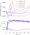 |
Fig. A.1. Time evolution of numerical errors (divB = 0, top panel) and the corresponding maximum cleaning potential Ψ (bottom panel). We present combinations of different κΨ and ch for a fixed κΦ = 1.0. |
As is lucidly shown in Fig. A.1, the introduction of the superluminal advection velocity ch into the augmented system of equations (Eq. (40)) for divergence cleaning reduces the error ε∇ ⋅ B (especially in the early and late phase of the evolution) significantly. Furthermore, the maximum magnitude of the cleaning potential Ψ decreases by two orders of magnitude. Small variations in ε∇ ⋅ B are also observed for stronger damping of errors by greater values for κΨ. Though the presented tests for flat background geometries employ ch = 1, we conclude from the results in Fig. A.1 that ch = 2 improves the code performance (i.e., reducing the arising numerical errors) for general relativistic spacetimes.
This comparison of parameters responsible for the cleaning of numerical errors emphasizes the strong need for a diligent calibration for each setup (i.e., boundary conditions, geometry, etc.) at hand. The standard configurations employed for the hyperbolic/parabolic cleaning of numerical errors should and will be readjusted in the light of future applications of our GRFFE method.
Appendix B: Conservation at refinement boundaries
Alfvén waves carry charge (and current). They are an excellent testbed for probing the conservative properties of a numerical method (cf. Mahlmann et al. 2021). In this section, we examine the quality of our conservative method at mesh refinement boundaries. We consider a (smoother) variation the degenerate Alfvén wave test from Komissarov (2002) and Yu (2011). For this, we boost the initial data given by Eq. (74) into a frame with β = 0.5:
![$$ \begin{aligned}&\mathbf B =\left(1,\sqrt{3},2B^z/\sqrt{3}\right),\qquad \mathbf D =\left(-B^z,-B^z/\sqrt{3},\sqrt{3}\right),\nonumber \\&B^z=\left\{ \begin{array}{cc} 1&x\le 0\\ 1+0.15\left[1+\sin \left[5\pi \left(x-0.1\right)\right]\right]&0 < x\le 0.2\\ 1.3&x>0.2 \end{array}\right. . \end{aligned} $$](/articles/aa/full_html/2021/03/aa38907-20/aa38907-20-eq124.gif)
Figure B.1 shows components of the electric and magnetic fields of the solution developed up to t = 2 on a uniform mesh (comparable to the respective tests in Komissarov 2002; Yu 2011). We then repeat this test with an additional level of refinement for x ≤ −0.25 and display the main results in Fig. B.2. The degenerate Alfvén wave thus crosses one mesh refinement boundary during its evolution.
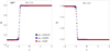 |
Fig. B.1. Degenerate Alfvén wave test on a x ∈ [−2,2] grid (fCFL = 0.25) at t = 2.0 and for different resolutions. The theoretically expected position of the Alfven wave is indicated by a gray dashed line. |
The quality of our conservative method for global quantities – such as the electric charge – is impaired on the level of an error of several percent if no refluxing is used (black line in the left panel of Fig. B.2). The same statement (though on a smaller scale) is also true for the energy, as we show in the right panel of Fig. B.2. If refluxing is used, on the other hand, energy is conserved up to machine precision or violation of the force-free conditions. Such levels of nonconservation in simple 1D tests justify the use of refluxing techniques (cf. Sect. 3), especially in highly dynamic 3D simulations.
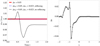 |
Fig. B.2. Same test as in Fig. B.1, but with an additional level of mesh refinement for x ≤ −0.25. Left: comparison of global charge conservation between a uniform grid (red line), a refined mesh with refluxing (blue line), and a refined grid without refluxing (black line). We display the relative deviation of the total charge from its initial value for different setups. Right: difference between the electromagnetic energy density for the refined mesh with and without refluxing at t = 2.0. |
All Figures
|
Fig. 1. Current sheet test (Komissarov 2004; Yu 2011) as described by the initial data in Eq. (72) on a x ∈ [−2,2] grid (fCFL = 0.25) at t = 1.0 for B0 = 0.5 and different resolutions. Two fast waves emerge from the original discontinuity and propagate outward with the speed of light (analytical position of the waves are indicated by dashed vertical lines). The order of convergence, 𝒪 is indicated according to Eq. (71). Top: MP7 reconstruction. Bottom: MC reconstruction. |
| In the text | |
|
Fig. 2. Degenerate current sheet test (Komissarov 2004; Yu 2011) as as described by the initial data (Eq. (72)) with B0 = 2.0. Two fast waves emerge from the original discontinuity and propagate outward with the speed of light. The cross field conductivity (induced by conserving conditions (37), and (38)) terminates the fast waves in the breakdown-zone. Top: MP7 reconstruction. Bottom: MC reconstruction. |
| In the text | |
|
Fig. 3. Same scenario as Fig. 2. The panels show the magnetic dominance state (cf. Fig. C2, Komissarov 2004). D2 > B2 develops at the location of the central current sheet, such that the electric field is altered by the algebraic adjustment maintaining condition (38). Our numerical implementation of the adjustment (63) drives D2 − B2 → 0 instantaneously, restoring magnetic dominance. |
| In the text | |
|
Fig. 4. Three-wave problem (Paschalidis & Shapiro 2013) as described by the setup in Eq. (73) and employing MP7 reconstruction. Numerical setup and labels are the same as in Fig. 1. The initial discontinuity at x = 0 splits into two fast discontinuities and one stationary Alfvén wave. |
| In the text | |
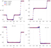 |
Fig. 5. Same as Fig. 4 but employing MC reconstruction. |
| In the text | |
|
Fig. 6. Stationary Alfvén wave problem (Komissarov 2004), same numerical setup as in Fig. 1. The analytic solution (Eq. 74) is indicated by a gray line. |
| In the text | |
|
Fig. 7. Free-energy U (normalized to its initial value U0) during the collision of Alfvén wave packets on numerical meshes (2D/3D) of various resolutions (indicated by different line styles). Top: evolution of U0/U for the set of 2D models. Slopes for the asymptotic linear relation between U0/U and ln t are indicated by dashed/dotted lines, comparing to Fig. 7 of Li et al. (2019). Bottom: free-energy evolution normalized to U0 comparing to Figs. 2 and 5 from Li et al. (2019). The asymptotic slope for 3D models found by Li et al. (2019) is indicated by a gray dashed line for reference. |
| In the text | |
|
Fig. 8. Spectrum evolution for the 2D simulation of Alfvén interactions initialized according to Eq. (78). We show the spectral energy distribution for wavenumbers k⊥ (perpendicular to the guide field) in analogy to Fig. 6, Li et al. (2019). Top: spectral energy distribution at different times for the resolution 5122. Bottom: spectral energy distribution for selected times and wavenumbers (color code as in top panel) and different resolutions, indicated by dashed (1282), dotted (2562) and solid (5122) lines. No visible convergence is reached. |
| In the text | |
|
Fig. 9. Spectrum evolution for the 3D simulation of Alfvén interactions initialized according to Eq. (75). We show the spectral energy distribution for wavenumbers k⊥ (perpendicular to the guide field) in analogy to Fig. 2, Li et al. (2019). Top: spectral energy distribution at different times for the resolution 3843. Bottom: spectral energy distribution for selected times and wavenumbers (color code as in top panel) and different resolutions, indicated by dashed (1283), dotted (2563) and solid (3843) lines. For wavenumbers k⊥ ≲ 40, convergence is reached for the shown high-resolution cases. |
| In the text | |
|
Fig. 10. Stability and relaxation test of magnetar magnetospheres endowed with an analytic dipole field structure for different resolutions. Upper panels: total magnetospheric energy normalized to the energy of the corresponding dipole. Lower panels: time derivative of the energy normalized to the dipole. The resolutions of 16 and 32 points per stellar radius in a 3D Cartesian CARPET grid (left) correspond to the setup in Mahlmann et al. (2019). Axially symmetric simulations in spherical coordinates (right) are set up with the indicated resolution at the stellar surface. Black (solid and dashed) lines in the upper-right panel correspond to a simulation on a smaller domain, extending up to r = 935.26 M⊙ − 6Δr, in which the pulses of the initial relaxation have sufficient time to leave the domain. |
| In the text | |
|
Fig. 11. Stability test of magnetar magnetospheres endowed with a tilted (30 degrees) analytic dipole field structure for different resolutions. Left: evolution of the l2-norm of the error with respect to the analytical (initial) configuration normalized to the magnetic field strength Bp at the magnetar pole (top), and of the total magnetospheric energy content (bottom). Right: 3D impression of the final state (t ≈ 1.5 ms) of the intermediate resolution simulation (Δr = R*/24). We display the magnetic field lines colorized by their norm. |
| In the text | |
|
Fig. 12. Force-free aligned rotator test in spherical ideal FFE for different resolutions. Left panel a: global structure of the magnetosphere for intermediate resolution (32 pts./r*). The poloidal fieldlines are indicated by black solid and dashed lines, depending on the magnetic field direction. Blue and red colors represent direction and magnitude of the toroidal magnetic field (normalized to its maximum value). Middle panel b: zoom on the Y-point and equatorial current sheet (alternating magnetic field highlighted by cyan field lines) for different resolutions. The color scale represents the current density (normalized to the current density of the low-resolution data). Left panel c: field line angular velocity measured at different radii. |
| In the text | |
|
Fig. 13. Time evolution of the Schwarzschild monopole (ΩF = ΩBH/2) of a slowly spinning Kerr BH (a* = 0.1, M = 1) in Cartesian (3D CARPET grid with nine refinement levels, with the highest resolution of 0.03125 M⊙ completely enclosing the central object) and spherical (2D, axsymmetric) coordinates. The spacetime metric is dynamically evolving. Left: evolution of the total magnetospheric (electromagnetic) energy normalized to the initial value, e0. Right: field line angular velocity along the equatorial plane. The final value is shown in a strong color. Intermediate states throughout the simulation are depicted by lighter colored lines (the strength of the color increasing with simulation time). |
| In the text | |
|
Fig. 14. Simulations of Wald magnetospheres for a* = 0.5 and M = 1 at t = 128 M⊙. Left: 3D Cartesian CARPET grid (vacuum spacetime modeled by MACLACHLAN). Right: 2D (axially symmetric) spherical grid (vacuum spacetime modeled by SPHERICALBSSN). The poloidal field is indicated by streamlines, the toroidal field by red and blue colors (color scale coincides for all panels) indicating whether the toroidal field leaves or enters into the displayed plane, respectively. The BH ergosphere is denoted by a solid white line. |
| In the text | |
|
Fig. 15. Simulations of a Wald magnetosphere for a* = 0.9 in Cartesian coordinates for t = 256 M⊙. Left: same format and color scale as in Fig. 14. Right: 3D magnetic field line impression of the Wald magnetosphere. Darker colors indicate a stronger twist of the magnetic field. |
| In the text | |
|
Fig. 16. One-dimensional values of the field line angular velocity (top) and the toroidal magnetic field (bottom) for the Wald test (Cartesian CARPET grid) at t = 256 M⊙ and using different BH dimensionless rapidities (see legends). The interpolation radius (for the extraction in a Cartesian grid) is indicated in the respective panel, corresponding to the ergosphere radius at the equator (top) or the BH horizon radius (bottom). |
| In the text | |
|
Fig. A.1. Time evolution of numerical errors (divB = 0, top panel) and the corresponding maximum cleaning potential Ψ (bottom panel). We present combinations of different κΨ and ch for a fixed κΦ = 1.0. |
| In the text | |
|
Fig. B.1. Degenerate Alfvén wave test on a x ∈ [−2,2] grid (fCFL = 0.25) at t = 2.0 and for different resolutions. The theoretically expected position of the Alfven wave is indicated by a gray dashed line. |
| In the text | |
|
Fig. B.2. Same test as in Fig. B.1, but with an additional level of mesh refinement for x ≤ −0.25. Left: comparison of global charge conservation between a uniform grid (red line), a refined mesh with refluxing (blue line), and a refined grid without refluxing (black line). We display the relative deviation of the total charge from its initial value for different setups. Right: difference between the electromagnetic energy density for the refined mesh with and without refluxing at t = 2.0. |
| In the text | |
Current usage metrics show cumulative count of Article Views (full-text article views including HTML views, PDF and ePub downloads, according to the available data) and Abstracts Views on Vision4Press platform.
Data correspond to usage on the plateform after 2015. The current usage metrics is available 48-96 hours after online publication and is updated daily on week days.
Initial download of the metrics may take a while.