| Issue |
A&A
Volume 646, February 2021
|
|
|---|---|---|
| Article Number | L12 | |
| Number of page(s) | 8 | |
| Section | Letters to the Editor | |
| DOI | https://doi.org/10.1051/0004-6361/202040097 | |
| Published online | 16 February 2021 | |
Letter to the Editor
Low surface brightness galaxies in z > 1 galaxy clusters: HST approaching the progenitors of local ultra diffuse galaxies
1
Ruhr University Bochum, Faculty of Physics and Astronomy, Astronomical Institute, Universitätsstr. 150, 44801 Bochum, Germany
e-mail: This email address is being protected from spambots. You need JavaScript enabled to view it.
2
European Southern Observatory, Karl-Schwarzschild-Str. 2, 85748 Garching, Germany
e-mail: This email address is being protected from spambots. You need JavaScript enabled to view it.
3
Univ. Lyon, ENS de Lyon, Univ. Lyon 1, CNRS, Centre de Recherche Astrophysique de Lyon, UMR5574, 69007 Lyon, France
e-mail: This email address is being protected from spambots. You need JavaScript enabled to view it.
4
Cosmic Dawn Center (DAWN), Copenhagen, Denmark
5
Niels Bohr Institute, University of Copenhagen, Lyngbyvej 2, 2100 Copenhagen, Denmark
6
Department of Physics and Astronomy, York University, 4700, Keele Street, Toronto, ON MJ3 1P3, Canada
Received:
9
December
2020
Accepted:
15
January
2021
Abstract
Ultra diffuse galaxies (UDGs) are a type of large low surface brightness (LSB) galaxies with particularly large effective radii (reff > 1.5 kpc) that are now routinely studied in the Local (z < 0.1) Universe. While they are found to be abundant in clusters, groups, and in the field, their formation mechanisms remain elusive and comprise an active topic of debate. New insights may be found by studying their counterparts at higher redshifts (z > 1.0), even though cosmological surface brightness dimming makes them particularly difficult to detect and study in this channel. In this work, we use the deepest Hubble Space Telescope (HST) imaging stacks of z > 1 clusters, namely, SPT-CL J2106−5844 and MOO J1014+0038. These two clusters, at z = 1.13 and z = 1.23, respectively, were monitored as part of the HST See-Change programme. In making a comparison with the Hubble Extreme Deep Field as the reference field, we find statistical over-densities of large LSB galaxies in both clusters. Based on stellar-population modelling and assuming no size evolution, we find that the faintest sources we can detect are about as bright as expected for the progenitors of the brightest local UDGs. We find that the LSBs we detect in SPT-CL J2106−5844 and MOO J1014−5844 already have old stellar populations that place them on the red sequence. In correcting for incompleteness and based on an extrapolation of local scaling relations, we estimate that distant UDGs are relatively under-abundant, as compared to local UDGs, by a factor ∼3. A plausible explanation for the implied increase over time would be the significant growth of these galaxies over the last ∼8 Gyr, as also suggested by hydrodynamical simulations.
Key words: galaxies: dwarf / galaxies: formation / galaxies: clusters: general
As part of the 1st ESO Summer Research Programme.
© ESO 2021
1. Introduction
Dwarf galaxies exhibit a vast range of properties in terms of size and luminosity. Twenty particularly large (10 kpc) dwarfs with low surface brightness (LSB) were discovered through extensive photometric studies of the Virgo cluster by Sandage & Binggeli (1984). An additional 27 examples were found in the Virgo cluster (Impey et al. 1988) as well as in the Fornax cluster (Ferguson & Sandage 1988). While these objects were found in high density environments, similar low surface brightness objects were also discovered in lower density environments, such as the field (Dalcanton et al. 1997; Román et al. 2019).
More recently, after discovering 47 similar LSB objects (reff ∼ 3−10″, or reff > 1.5 kpc, and μ(g, 0) = 24−26 mag arcsec−2) in the Coma cluster, the term ‘ultra diffuse galaxies’ (UDGs) was introduced for these objects (van Dokkum et al. 2015a). Due to their projected density and their spatial coincidence with the Coma cluster, van Dokkum et al. (2015a) concluded that these objects are a part of the Coma cluster, which was later confirmed via a follow-up spectroscopic study (van Dokkum et al. 2015b).
Although obtaining redshift measurements of sizable samples of UDGs still poses a challenge, their overdensity in galaxy clusters allows us to study their properties in such over-dense environments. An approximately linear dependence between the abundance of UDGs in galaxy clusters and the cluster mass was found (van der Burg et al. 2017; Janssens et al. 2017; Román & Trujillo 2017). Within clusters, UDGs appear to be found on the red sequence (van Dokkum et al. 2015a; van der Burg et al. 2016), while UDG-like galaxies found in the field typically appear to be bluer (Leisman et al. 2017; Prole et al. 2019).
Important open questions surrounding the study of UDGs are related to their origin, for which different theories have been proposed in the literature. In particular, van Dokkum et al. (2015a) suggested that (some) UDGs may have formed in halos with masses similar to the Milky Way, but which ‘failed’ to form an L* galaxy. Also, UDGs may present extremes in a continuous distribution in dwarf galaxy properties, having acquired their expanded sizes due to internal (Amorisco & Loeb 2016; Di Cintio et al. 2017) or external (Bennet et al. 2018) processes.
Given the suggested low dark-matter content of some field UDGs (van Dokkum et al. 2018), it is also possible that they may also have formed as tidal dwarf galaxies (Bennet et al. 2018; Fensch et al. 2019). Since these formation processes happen over different time scales, observing the evolving properties of UDGs may help distinguish between different scenarios. To this end, we searched for LSB galaxies in the two galaxy clusters SPTCL-2106-5844 (z = 1.13) and MOO-1014+0038 (z = 1.23). Using deep HST image stacks for those clusters, we reached the spatial resolution required to measure their sizes. Here, we discuss our results in the context of the UDGs found in the Local Universe.
This Letter is organised as follows. Section 2 provides an overview of the data we used. Section 3 describes how we select our sample of UDGs. In Sect. 4, we discuss our results on the abundance and colour of the sample. We present our summary in Sect. 5. We adopt the ΛCDM cosmology with Ωm = 0.3, ΩΛ = 0.7, and H0 = 70 km s−1 Mpc−1. At the redshift of our clusters, 1 arcsec corresponds to ∼8.2−8.4 kpc. For the stellar masses, we assume the initial mass function (IMF) from Chabrier (2003). All magnitudes cited are in the AB magnitude system.
2. Data
In this study, we make use of HST photometry taken as part of the See-Change programme (HST GO 13677, 14327; PI: Perlmutter), which targets galaxy clusters in the range of 1.13 < z < 1.75. The main goal of the programme is to find high-z supernovae (SN) type Ia and to use these objects to constrain the expansion rate of the universe. The survey strategy has therefore been to take data with a roughly monthly cadence (e.g., Williams et al. 2020). Rather than using the individual exposures, here we use the image stacks, which reach a combined exposure time from 3.99 to 5.13 h in F140W per cluster we examined. In this work, we focus on the two lowest-z clusters from their sample.
The first cluster we analysed is SPT-CL J2106−5844 (hereafter, SPTCL-2106) at redshift z = 1.13. It was discovered with the South Pole Telescope (SPT) thanks to its strong Sunyaev-Zel’dovich effect (SZ) signal, yielding a mass estimate of M200 = (1.27 ± 0.21) × 1015 M⊙ (Foley et al. 2011). The second cluster is MOO J1014+0038 (MOO-1014) at redshift z = 1.23, discovered by the Massive and Distant Clusters of WISE Survey (MaDCoWS) based on a rich overdensity of galaxies (Gonzalez et al. 2019). It has a mass estimate of M200 = (5.6 ± 0.6) × 1014 M⊙ and a strong SZ signature (Brodwin et al. 2015). The RGB images of the two clusters are shown in Figs. A.1 and A.2.
To create full-depth mosaics of both clusters, we started by aligning each of the multiple SN monitoring ‘visits’ first internally to a catalogue of sources detected in a single F140W visit and then globally to sources matched in the Gaia DR2 catalogue (Gaia Collaboration 2018). We used the ASTRODRIZZLE software package (Gonzaga et al. 2012) to identify and mask cosmic rays and bad pixels in the aligned individual exposures and to perform source detection on the final combined F140W (WFC3/IR) mosaic generated with 60 mas pixels. We further used the F814W (WFC3/UVIS) stacks to provide basic colour information (or limits on the inferred colour based on the F814W detection limit). The combination of these filters bridge the 4000 Å break at the redshifts of our clusters, thus providing clues on stellar populations and on devising ways to help in assessing the sample purity.
2.1. Reference field
To estimate the level of contamination of the sample by foreground and background objects, we require a field survey with the same filter bands and image depth. We therefore utilised the data stacks taken in the Hubble eXtreme Deep Field1 (XDF). These deep stacks are composed of data from 19 different HST programs covering the Hubble Ultra Deep Field from 2002 to 2012. For details on the data reduction we refer to Illingworth et al. (2013). To ensure similar source detection limits as for the clusters, we added artificial noise, so that the recovered fraction of simulated sources were similar between the reference and cluster fields (see Sect. 3.3).
3. Analysis
3.1. Source detection
Sources were detected by running SExtractor (Bertin & Arnouts 1996) on the F140W images of the clusters and the XDF. The parameters used to ensure optimal detection of faint and extended sources in the clusters can be found in Appendix B and an identical setup was used for the XDF images. We only considered sources in the relatively central regions of the cluster stacks, where exposure time is nearly uniform (cf. Figs. A.1 and A.2). Examples of detected objects in each of the two clusters are shown Fig. 1.
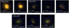 |
Fig. 1. RGB (red = F140W, green = F105W, blue = F814W) images of members of the studied clusters. Top: two spectroscopically-confirmed bright members of SPTCL-2106 (on the left) and three LSB galaxies that are likely members of SPTCL-2106 (based on a reference field comparison, on the right). Bottom: three LSB galaxies that are likely members of the cluster MOO-1014 (based on a reference field comparison). |
3.2. Structural parameters
For the detected sources, structural parameters such as magnitude, radius, ellipticity, and the Sérsic index of the detected objects were determined using GALFIT (Peng et al. 2002) on the F140W image after masking neighbouring objects detected by SExtractor. Here, GALFIT is also allowed to simultaneously fit a constant value to the sky background to improve the overall fit. In order to measure reliable colours, the F814W fluxes of the detected objects are measured on the corresponding stack by forcing GALFIT to use the morphological parameters obtained from the F140W stack and only fit the flux normalisation.
To estimate the measurement uncertainty, the GALFIT models were injected into a hundred different random locations in the corresponding cluster, with the requirement that there were no prior detections and they measured exactly as before. In this way, the 1-σ-uncertainties for size and magnitude in F140W and magnitude in F814W were obtained. We note that GALFIT measured a slightly lower flux (by about 0.2 mag) and smaller size (by about 0.3 kpc) than the simulated inputs. In the following, we correct for this small bias.
3.3. Image simulations
To assess the completeness of our UDG progenitor selection, we also performed all processing steps on a range of image simulations. For this purpose, we injected objects with Sérsic profiles into random locations in the HST stacks. We chose a constant Sérsic-n parameter of unity, which corresponds to typical light profiles of UDGs measured in the Local Universe (e.g., van Dokkum et al. 2015a; Koda et al. 2015; van der Burg et al. 2016). Sizes are drawn uniformly between  and
and  , and ellipticities, f, defined as f = 1 − b/a, with b/a the axis ratio, uniformly between 0.0 and 0.2. Each step was performed identically on the cluster image and on the reference field image.
Figure 2 shows the recovered fractions of the inserted objects for the two clusters and the reference field. While the detection limits in the different panels appear similar overall, we note that there is a substantial difference between the clusters and the reference field. Even for relatively bright sources, the recovery fraction is lower in the cluster than in the field. This is expected given the relatively high number of large and bright sources crowding the cluster stacks. These recovery fractions are used to determine the limits of our analysis, and to correct the detected sources for incompleteness, both due to limiting depth and due to crowding or obscuration.
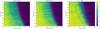 |
Fig. 2. Left: recovery fractions for the simulated sources in SPTCL-2106. Middle: same for MOO-1014. Right: same for the XDF reference field, with noise level matched to the cluster fields. The colour bar shows the recovery fractions. While the detection limits are comparable between the panels, the XDF shows overall a better recovery fraction for brighter targets than in the clusters due to a higher source crowding in the cluster fields. We also highlight the regime of objects with a surface brightness from 24.0 to 26.5 mag arcsec−2 in F140W and a radius from 1.5 to 7.0 kpc. |
3.4. Sample selection
While the definition of UDGs is rather arbitrary, we initially filter the sample by using a definition similar to that used in the Local Universe.
The surface brightness in F140W has to be fainter than 24.0 mag arcsec−2 (i.e. not corrected for surface brightness dimming) and the effective radius has to be between 1.5 and 7.0 kpc. Additionally the Sérsic index has to be smaller than 4.0 to increase the sample purity in favour of sources reminiscent of UDGs in the Local Universe and the distance between the SExtractor detection and the GALFIT position of measurement has to be smaller than 3.0 pixels to ensure that both relate to the same object. A fainter limit for the surface brightness is not included since one purpose of the study is to test the detection limits of LSB galaxies with the available data. After detecting sources in the direction of the clusterm we assume that each source is at the redshift of the cluster to infer their physical parameters. This is a valid assumption since we subsequently performed a statistical subtraction of fore- and background objects, thereby making the same assumption for sources detected in the reference field.
After discarding failed detections with a by-eye scan, we found 95 objects (10 discarded) in SPTCL-2106 (70 in the reference field, 6 discarded) and 111 objects (10 discarded) in MOO-1014 (72 in the reference field, 9 discarded). We note that the number of objects in the reference field depends on the assumed angular diameter distance and, thus, the redshift of the cluster. We conservatively only considered sources that would have had a detection probability of at least 50% in the reference field for both cluster and reference field objects and we only count the objects above this limit to ensure a reasonable completeness correction. For the remaining sources, we applied a completeness correction that is based on the determined recovery fractions by at most a factor of 2 (see Sect. 3.3). We also applied a correction based on the different sky area covered by the cluster and reference field. We are left with a statistical count of 99 ± 10 objects in SPTCL-2106 (67 ± 8 in reference field) and 90 ± 10 in MOO-1014 (70 ± 8 in reference field).
The colour-magnitude diagrams for all the detected sources falling within the 50%-limit (see Fig. C.1) in both the clusters and the reference field are shown in the Appendix C. We subtract the reference field galaxies from the nearest cluster object in regards of colour (F814W − F140W) and magnitude (F140W). For this, we use the colour and magnitude measurements for each cluster object as coordinates and subtract the reference field object from the nearest cluster object. The relative weights, which include corrections for incompleteness and different covered sky areas, are taken into account. For more details on the subtraction of the reference field, we refer to van der Burg et al. (2016). After subtraction, we are left with a statistical count of 32 ± 13 in SPTCL-2106 and 20 ± 13 in MOO-1014.
4. Results and discussion
4.1. Comparison with local UDGs
To feasibly compare our LSB candidates to likely progenitors of UDGs studied in the Local Universe, we evolved local UDGs back to the redshift of our clusters following a simple stellar population model. The model assumes a passively evolving stellar population that was formed at zform = 1.5, which is in line with the intermediately old ages of UDGs measured locally (Ferré-Mateu et al. 2018; Ruiz-Lara et al. 2018; Fensch et al. 2019). It is based on stellar population synthesis models from Bruzual & Charlot (2003), a star formation history, SFR ∝ e−t/τ, with a short e-folding time of τ = 10 Myr, a Chabrier (2003) initial mass function and no dust extinction. We use the magnitudes, physical sizes, and filters of van Dokkum et al. (2015a) as an anchor point and estimate how those UDGs would appear at the redshift of our cluster as observed through the WFC3/F140W filter. This estimate accounts, by construction, for surface brightness dimming. The 47 UDG candidates are shown in Fig. 3. Additionally, we evolved the dwarf and giant galaxies found by Mobasher et al. (2001) in the Coma cluster back to the redshift of our clusters in the same way and also plotted them in Fig. 3.
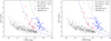 |
Fig. 3. Selection by size and apparent magnitude in F140W of our LSB galaxies. The panels show the different clusters. Red: LSB galaxies detected following our selection criteria and with a weight higher than 0.5. Blue and grey: samples from van Dokkum et al. (2015a) and Mobasher et al. (2001), both shifted to our observed redshift by accounting for an E+K correction (see Sect. 4). We plot curves of constant surface brightness, μ(reff, circ) = 24.0, 26.0 mag arcsec−2 evolved from the Coma cluster redshift to the high-z clusters. Average error bars for our sample are shown. |
Figure 3 shows that the LSB samples of our clusters lie in the area between the samples from van Dokkum et al. (2015a) and Mobasher et al. (2001), making them fainter than the progenitors of normal dwarf and giant galaxies in the Coma cluster, and almost as faint as the expected progenitors of the UDGs studied by van Dokkum et al. (2015a). We can see a small overlap between our samples and the compared objects from both other studies. As a reference, we also plot the curves of constant surface brightness, μ(r, reff, circ) = 24.0, 26.0 mag arcsec−2, which is a common selection boundary for UDGs in the Local Universe, also evolved to the redshifts of our clusters. This indicates that only half of the objects we are able to detect in both clusters could be classified as progenitors of the brightest UDGs known in the Local Universe, based on this evolution model.
We note that in projecting the local Coma galaxies back to higher redshift, we only evolved their fluxes and ignored any potential size evolution. However, numerical simulations suggest that a typical UDG may see its radius increase with age from around 2.5−3 kpc at z = 1 to 4−5 kpc at z = 0 (Martin et al. 2019; Wright et al. 2021). Accounting for such an expansion would bring the data points from van Dokkum et al. (2015a), when evolved to the redshift of our clusters downward and, thus, closer to our data points. A possible size evolution is described in Sect. 4.3 and the sample from van Dokkum et al. (2015a) that is affected by it is plotted in Fig. 4.
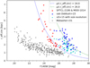 |
Fig. 4. Same as in Fig. 3 but for both clusters combined with the sample by van Dokkum et al. (2015a) and with the size evolution taken out. Cyan: sample from van Dokkum et al. (2015a), where the suggested size evolution since z ∼ 1 (cf. Sect. 4.3) is removed. |
4.2. Colour
Figure 5 shows the colours and magnitudes of the sample of LSB galaxies. The residual weight shows the number of galaxies we expect in the observed cluster area per detected object after accounting for the subtraction of the reference field. Also shown in Fig. 5 are the positions in the colour-magnitude diagram of galaxies that were spectroscopically confirmed as members of SPTCL-2106 (by the GOGREEN Collaboration, Balogh et al. 2021). The colours were measured in the same filter bands and following an identical method as for the LSB candidates. Ignoring some of the data points that may be part of a bluer, star-forming cluster population, we note that the bulk of the LSB galaxies lie on an extended red sequence, shown as a pink-dashed line, as defined by the brighter cluster galaxies. We note that the slope of this estimate red-sequence, −0.12, is consistent with the z ∼ 1 estimates from, for instance, Bell et al. (2004). No similar population of bright cluster members has been spectroscopically identified for MOO-1014, so we plot the same red-sequence estimate for this cluster, ignoring the small redshift difference between the two clusters. The LSB galaxies of SPTCL-2106 and MOO-1014 exhibit colours that are consistent with the red sequence, suggesting that these galaxies are likely to be quenched and have thus already ceased their star formation.
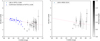 |
Fig. 5. Colour-magnitude diagrams for the sample of LSB candidates in the clusters after correcting for fore- and background interlopers and incompleteness. The colour bar gives the residual weight of the data points (as detailed in Sect. 3.4). Left panel: cluster SPTCL-2106, right panel: cluster MOO-1014. Additionally shown in the left panel, we have the positions in the colour-magnitude diagram of spectroscopically confirmed members of SPTCL-2106 and an extrapolation of the red sequence as defined by the confirmed members of SPTCL-2106, ignoring some of the data points that may be part of a bluer or star-forming cluster population to guide the reader’s eye. This line has a slope of −0.12. |
4.3. Abundance comparison with Local Universe UDGs
To set the measured abundance of LSB galaxies in our clusters in context, we compare it to the abundance of UDGs in local clusters, within a projected R < R200. For this purpose, we have to make assumptions regarding the underlying magnitude and size distribution of dwarf galaxies and consider how these aspects evolve with redshift. We assume a flat magnitude distribution for different size bins (consistent with what is observed in the Coma cluster, by Danieli & van Dokkum 2019) and the same size distribution as measured for UDGs in local clusters (for radii between 1.5 and 7.0 kpc, van der Burg et al. 2016). Based on Fig. 2, we can also assume that our samples in the range with surface brightness from 24.0 to 26.5 mag in F140W and a radius from 1.5 to 7.0 kpc are mostly complete for the parameter range studied of both clusters.
The available HST imaging does not allow us to probe radii out to R200, but only to radii corresponding to ∼0.35 ⋅ R200 for SPTCL-2106 and ∼0.50 ⋅ R200 for MOO-1014. To correct for the missing area, we assume that LSBs approximately trace the overall matter distribution in the cluster, which is described by an Navarro-Frenk-White (NFW; Navarro et al. 1997) profile with concentration c200 = 3 (e.g., Duffy et al. 2008). Integrating this profile along the line-of-sight indicates that we probe a fraction of ∼0.4 ± 0.1 of the LSB population in SPTCL-2106 and ∼0.55 ± 0.1 in MOO-1014. Based on the assumed magnitude and size distribution2, and after applying the needed correction for missed area, we go on to estimate a total number of 80 ± 38 UDGs in SPTCL-2106 and 36 ± 25 UDGs in MOO-1014. Studies of local clusters suggest an abundance of ∼100−200 in clusters of this mass, being three times higher than our best estimate for the clusters we study in this work. Thus, this implies a substantial increase in the UDG abundance with time since z ∼ 1. A possible explanation for this implied evolution is that we are assuming the UDG progenitors to be of the same size as Local Universe UDGs. If their progenitors were actually smaller at z = 1 (as suggested by several simulations, cf. Martin et al. 2019; Wright et al. 2021), they would not fall into our selection criteria and, thus, would be missed in the current analysis.
Assuming the size distribution of UDGs in the Local Universe, as described by the power law shown in Fig. 7 of van der Burg et al. (2016), we find that a size growth by a factor ∼1.4 of all galaxies may have boosted the number of galaxies classified as UDGs by a factor of ∼3 since z ∼ 1. Hydrodynamical simulations by Martin et al. (2019) would predict a slightly larger size growth by a factor ∼1.8. This suggests that size evolution can sufficiently explain the observed under-abundance of UDGs.
5. Summary and outlook
In this work, we study the abundance of LSB galaxies in two z > 1 clusters, SPTCL-2106 and MOO-1014, down to the detection limit of the available deep HST imaging data. We correct for background objects by comparing the detections with those measured in the XDF as the reference field. Simulations were run to estimate completeness limits and to tailor the depth of the reference field to the cluster imaging. We summarise our main conclusions as follows:
-
Within the parameter space we defined, we find a statistical overdensity of 32 ± 13 LSB galaxies in SPTCL-2106 and 20 ± 13 in MOO-1014.
-
We find the colours of those LSB galaxies in SPTCL-2106 and MOO-1014 to be consistent with an extension of the red sequence, as defined by spectroscopically identified brighter cluster members. This suggests that the LSB galaxies in both clusters are already evolving passively.
-
Based on a simple stellar population evolution model, we compared our detected LSB galaxies with the expected progenitors of local UDGs in the Coma cluster. This suggests that the faintest sources we can detect approximate the expected progenitors of local UDGs.
-
Based on an extrapolation, motivated by local scaling relations, we estimate an overall abundance of 80 ± 38 UDGs in SPTCL-2106 and 36 ± 25 UDGs in MOO-1014. We note that this is about three times lower than the abundance of UDGs in local galaxy clusters having similar masses.
-
One way to interpret the implied evolution is to assume a substantial size growth on the part of dwarf galaxies since z ∼ 1, which would then increase the numbers of those classified as UDGs. As we discuss here, this is qualitatively consistent with the results from the relevant hydrodynamical simulations.
We emphasise that in this study, we use the deepest data available for galaxy clusters at z > 1 that still allow us to spatial resolve galaxies of 1−2 kpc, thus reaching the limits of the instrumentation that is currently available. For further studies on the existence and properties of distant UDGs, data with higher spatial resolution and depth is needed, a requirement that is within reach of the next generation of telescopes.
We considered uncertainties in the assumed size distribution (as measured in van der Burg et al. 2016) and magnitude distribution (as measured in Danieli & van Dokkum 2019), finding that these affect our estimated number of high-z UDGs by at most 14%, hence not impacting our conclusions.
Acknowledgments
We thank the anonymous referee for their useful comments that substantially clarified the paper. AB acknowledges a 6-week ESO summer studentship during which a substantial part of this research was done.
References
- Amorisco, N. C., & Loeb, A. 2016, MNRAS, 459, L51 [NASA ADS] [CrossRef] [Google Scholar]
- Balogh, M. L., van der Burg, R. F. J., Muzzin, A., et al. 2021, MNRAS, 500, 358 [CrossRef] [Google Scholar]
- Bell, E. F., Wolf, C., Meisenheimer, K., et al. 2004, ApJ, 608, 752 [NASA ADS] [CrossRef] [Google Scholar]
- Bennet, P., Sand, D. J., Zaritsky, D., et al. 2018, ApJ, 866, L11 [NASA ADS] [CrossRef] [Google Scholar]
- Bertin, E., & Arnouts, S. 1996, A&AS, 117, 393 [NASA ADS] [CrossRef] [EDP Sciences] [Google Scholar]
- Brodwin, M., Greer, C. H., Leitch, E. M., et al. 2015, ApJ, 806, 26 [NASA ADS] [CrossRef] [Google Scholar]
- Bruzual, G., & Charlot, S. 2003, MNRAS, 344, 1000 [NASA ADS] [CrossRef] [Google Scholar]
- Chabrier, G. 2003, PASP, 115, 763 [Google Scholar]
- Dalcanton, J. J., Spergel, D. N., Gunn, J. E., Schmidt, M., & Schneider, D. P. 1997, AJ, 114, 635 [Google Scholar]
- Danieli, S., & van Dokkum, P. 2019, ApJ, 875, 155 [CrossRef] [Google Scholar]
- Di Cintio, A., Tremmel, M., Governato, F., et al. 2017, MNRAS, 469, 2845 [CrossRef] [Google Scholar]
- Duffy, A. R., Schaye, J., Kay, S. T., & Dalla Vecchia, C. 2008, MNRAS, 390, L64 [NASA ADS] [CrossRef] [Google Scholar]
- Fensch, J., van der Burg, R. F. J., Jeřábková, T., et al. 2019, A&A, 625, A77 [NASA ADS] [CrossRef] [EDP Sciences] [Google Scholar]
- Ferguson, H. C., & Sandage, A. 1988, AJ, 96, 1520 [NASA ADS] [CrossRef] [Google Scholar]
- Ferré-Mateu, A., Alabi, A., Forbes, D. A., et al. 2018, MNRAS, 479, 4891 [NASA ADS] [CrossRef] [Google Scholar]
- Foley, R. J., Andersson, K., Bazin, G., et al. 2011, ApJ, 731, 86 [NASA ADS] [CrossRef] [Google Scholar]
- Gaia Collaboration (Brown, A. G. A., et al.) 2018, A&A, 616, A1 [NASA ADS] [CrossRef] [EDP Sciences] [Google Scholar]
- Gonzaga, S., Hack, W., Fruchter, A., et al. 2012, The DrizzlePac Handbook, HST Data Handbook [Google Scholar]
- Gonzalez, A. H., Gettings, D. P., Brodwin, M., et al. 2019, ApJS, 240, 33 [NASA ADS] [CrossRef] [Google Scholar]
- Illingworth, G. D., Magee, D., Oesch, P. A., et al. 2013, ApJS, 209, 6 [Google Scholar]
- Impey, C., Bothun, G., & Malin, D. 1988, ApJ, 330, 634 [Google Scholar]
- Janssens, S., Abraham, R., Brodie, J., et al. 2017, ApJ, 839, L17 [NASA ADS] [CrossRef] [Google Scholar]
- Koda, J., Yagi, M., Yamanoi, H., & Komiyama, Y. 2015, ApJ, 807, L2 [NASA ADS] [CrossRef] [Google Scholar]
- Leisman, L., Haynes, M. P., Janowiecki, S., et al. 2017, ApJ, 842, 133 [NASA ADS] [CrossRef] [Google Scholar]
- Martin, G., Kaviraj, S., Laigle, C., et al. 2019, MNRAS, 485, 796 [NASA ADS] [CrossRef] [Google Scholar]
- Mobasher, B., Bridges, T. J., Carter, D., et al. 2001, ApJS, 137, 279 [NASA ADS] [CrossRef] [Google Scholar]
- Navarro, J. F., Frenk, C. S., & White, S. D. M. 1997, ApJ, 490, 493 [NASA ADS] [CrossRef] [Google Scholar]
- Peng, C. Y., Ho, L. C., Impey, C. D., & Rix, H.-W. 2002, AJ, 124, 266 [Google Scholar]
- Prole, D. J., van der Burg, R. F. J., Hilker, M., & Davies, J. I. 2019, MNRAS, 488, 2143 [NASA ADS] [Google Scholar]
- Román, J., & Trujillo, I. 2017, MNRAS, 468, 4039 [Google Scholar]
- Román, J., Beasley, M. A., Ruiz-Lara, T., & Valls-Gabaud, D. 2019, MNRAS, 486, 823 [NASA ADS] [CrossRef] [Google Scholar]
- Ruiz-Lara, T., Beasley, M. A., Falcón-Barroso, J., et al. 2018, MNRAS, 478, 2034 [NASA ADS] [CrossRef] [Google Scholar]
- Sandage, A., & Binggeli, B. 1984, AJ, 89, 919 [Google Scholar]
- van der Burg, R. F. J., Muzzin, A., & Hoekstra, H. 2016, A&A, 590, A20 [NASA ADS] [CrossRef] [EDP Sciences] [Google Scholar]
- van der Burg, R. F. J., Hoekstra, H., Muzzin, A., et al. 2017, A&A, 607, A79 [NASA ADS] [CrossRef] [EDP Sciences] [Google Scholar]
- van Dokkum, P. G., Abraham, R., Merritt, A., et al. 2015a, ApJ, 798, L45 [NASA ADS] [CrossRef] [Google Scholar]
- van Dokkum, P. G., Romanowsky, A. J., Abraham, R., et al. 2015b, ApJ, 804, L26 [NASA ADS] [CrossRef] [Google Scholar]
- van Dokkum, P., Danieli, S., Cohen, Y., et al. 2018, Nature, 555, 629 [NASA ADS] [CrossRef] [Google Scholar]
- Williams, S. C., Hook, I. M., Hayden, B., et al. 2020, MNRAS, 495, 3859 [CrossRef] [Google Scholar]
- Wright, A. C., Tremmel, M., Brooks, A. M., et al. 2021, MNRAS, in press [arXiv:2005.07634] [Google Scholar]
Appendix A: RGB images of the clusters
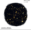 |
Fig. A.1. RGB (red = F140W, green = F105W, blue = F814W) image of the cluster SPTCL-2106. |
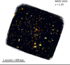 |
Fig. A.2. RGB (red = F140W, green = F105W, blue = F814W) image of the cluster MOO-1014. |
Appendix B: SExtractor parameters
SExtractor parameters used. All other parameters were left to their defaults.
Appendix C: Additional figure
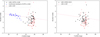 |
Fig. C.1. Colour-magnitude diagrams for the sample of LSB candidates in the clusters and the reference field that fall within the 50% detection limit. These are the raw numbers, without accounting for incompleteness or background interlopers. Left panel: cluster SPTCL-2106, right panel: cluster MOO-1014. Additionally shown in the left panel, we have the positions in the colour-magnitude diagram of spectroscopically-confirmed members of SPTCL-2106 and the same extrapolation of the red-sequence as described in Fig. 5. |
All Tables
All Figures
|
Fig. 1. RGB (red = F140W, green = F105W, blue = F814W) images of members of the studied clusters. Top: two spectroscopically-confirmed bright members of SPTCL-2106 (on the left) and three LSB galaxies that are likely members of SPTCL-2106 (based on a reference field comparison, on the right). Bottom: three LSB galaxies that are likely members of the cluster MOO-1014 (based on a reference field comparison). |
| In the text | |
|
Fig. 2. Left: recovery fractions for the simulated sources in SPTCL-2106. Middle: same for MOO-1014. Right: same for the XDF reference field, with noise level matched to the cluster fields. The colour bar shows the recovery fractions. While the detection limits are comparable between the panels, the XDF shows overall a better recovery fraction for brighter targets than in the clusters due to a higher source crowding in the cluster fields. We also highlight the regime of objects with a surface brightness from 24.0 to 26.5 mag arcsec−2 in F140W and a radius from 1.5 to 7.0 kpc. |
| In the text | |
|
Fig. 3. Selection by size and apparent magnitude in F140W of our LSB galaxies. The panels show the different clusters. Red: LSB galaxies detected following our selection criteria and with a weight higher than 0.5. Blue and grey: samples from van Dokkum et al. (2015a) and Mobasher et al. (2001), both shifted to our observed redshift by accounting for an E+K correction (see Sect. 4). We plot curves of constant surface brightness, μ(reff, circ) = 24.0, 26.0 mag arcsec−2 evolved from the Coma cluster redshift to the high-z clusters. Average error bars for our sample are shown. |
| In the text | |
|
Fig. 4. Same as in Fig. 3 but for both clusters combined with the sample by van Dokkum et al. (2015a) and with the size evolution taken out. Cyan: sample from van Dokkum et al. (2015a), where the suggested size evolution since z ∼ 1 (cf. Sect. 4.3) is removed. |
| In the text | |
|
Fig. 5. Colour-magnitude diagrams for the sample of LSB candidates in the clusters after correcting for fore- and background interlopers and incompleteness. The colour bar gives the residual weight of the data points (as detailed in Sect. 3.4). Left panel: cluster SPTCL-2106, right panel: cluster MOO-1014. Additionally shown in the left panel, we have the positions in the colour-magnitude diagram of spectroscopically confirmed members of SPTCL-2106 and an extrapolation of the red sequence as defined by the confirmed members of SPTCL-2106, ignoring some of the data points that may be part of a bluer or star-forming cluster population to guide the reader’s eye. This line has a slope of −0.12. |
| In the text | |
|
Fig. A.1. RGB (red = F140W, green = F105W, blue = F814W) image of the cluster SPTCL-2106. |
| In the text | |
|
Fig. A.2. RGB (red = F140W, green = F105W, blue = F814W) image of the cluster MOO-1014. |
| In the text | |
|
Fig. C.1. Colour-magnitude diagrams for the sample of LSB candidates in the clusters and the reference field that fall within the 50% detection limit. These are the raw numbers, without accounting for incompleteness or background interlopers. Left panel: cluster SPTCL-2106, right panel: cluster MOO-1014. Additionally shown in the left panel, we have the positions in the colour-magnitude diagram of spectroscopically-confirmed members of SPTCL-2106 and the same extrapolation of the red-sequence as described in Fig. 5. |
| In the text | |
Current usage metrics show cumulative count of Article Views (full-text article views including HTML views, PDF and ePub downloads, according to the available data) and Abstracts Views on Vision4Press platform.
Data correspond to usage on the plateform after 2015. The current usage metrics is available 48-96 hours after online publication and is updated daily on week days.
Initial download of the metrics may take a while.