| Issue |
A&A
Volume 646, February 2021
|
|
|---|---|---|
| Article Number | A4 | |
| Number of page(s) | 11 | |
| Section | Planets and planetary systems | |
| DOI | https://doi.org/10.1051/0004-6361/202040066 | |
| Published online | 02 February 2021 | |
Planet cartography with neural learned regularization
1
Instituto de Astrofísica de Canarias (IAC),
Avda Vía Láctea S/N,
38200 La Laguna,
Tenerife, Spain
e-mail: This email address is being protected from spambots. You need JavaScript enabled to view it.
2
Departamento de Astrofísica, Universidad de La Laguna,
38205 La Laguna,
Tenerife, Spain
Received:
4
December
2020
Accepted:
10
December
2020
Abstract
Aims. Finding potential life harboring exo-Earths with future telescopes is one of the aims of exoplanetary science. Detecting signatures of life in exoplanets will likely first be accomplished by determining the bulk composition of the planetary atmosphere via reflected or transmitted spectroscopy. However, a complete understanding of the habitability conditions will surely require mapping the presence of liquid water, continents, and/or clouds. Spin-orbit tomography is a technique that allows us to obtain maps of the surface of exoplanets around other stars using the light scattered by the planetary surface.
Methods. We leverage the enormous potential of deep learning, and propose a mapping technique for exo-Earths in which the regularization is learned from mock surfaces. The solution of the inverse mapping problem is posed as a deep neural network that can be trained end-to-end with suitable training data. Since we still lack observational data of the surface albedo of exoplanets, in this work we propose methods based on the procedural generation of planets, inspired by what we have found on Earth. We also consider mapping the recovery of surfaces and the presence of persistent clouds in cloudy planets, a much more challenging problem.
Results. We show that reliable mapping can be carried out with our approach, producing very compact continents, even when using single-passband observations. More importantly, if exoplanets are partially cloudy like the Earth is, we show that it is possible to map the distribution of persistent clouds that always occur in the same position on the surface (associated with orography and sea surface temperatures) together with nonpersistent clouds that move across the surface. This will become the first test to perform on an exoplanet for the detection of an active climate system. For small rocky planets in the habitable zone of their stars, this weather system will be driven by water, and the detection can be considered a strong proxy for truly habitable conditions.
Key words: methods: numerical / planets and satellites: surfaces / planets and satellites: terrestrial planets
© ESO 2021
1 Introduction
One of the most promising goals in the field of exoplanets is to reach the technical capability to characterize the bulk composition of rocky exoplanet atmospheres, in particular of those small planets within the habitable zone of their host star, which will in turn open the search to the combination of gaseous species that could be classified as a biomarker (Des Marais et al. 2002). With more than 4000 planets detected to date, the number of small rocky planets is also large, and it continues to increase thanks to space missions like Kepler and TESS, as well as ground-based photometric and radial velocity surveys. The majority of these small rocky planets, however, transit around M-type stellar hosts (Hardegree-Ullman et al. 2019). This is good news as these small stars offer a greater chance of planetary characterization owing to a reduced star/planet contrast ratio. In the near future, ultra-stable high resolution spectrographs, such as ESPRESSO, mounted on large aperture telescopes, such as the Extremely Large Telescope (ELT) will allow the detection of small rocky planets around K- and G-type stars.
The initial characterization of small rocky planets will probably be performed by transmission spectroscopy of targets around M-type stars (Pallé et al. 2011; Snellen et al. 2013), although whether these planets can sustain an atmosphere or host life is still open to debate (Tarter et al. 2007; Luger & Barnes 2015). In the longer term, direct imaging of habitable zone exoplanets will be accomplished by space-based coronographic or interferometric techniques (Léger et al. 1996). This expansion into reflected light studies is crucial for our understanding of planetary atmospheres (and possible biomarkers) in the solar neighborhood as for an Earth–Sun twin the transit probability is only 0.5%, meaning that only one of the 200 closest Earth-like planets will transit its host star.
Characterizing planets via reflected light poses a technical challenge, but it also offers the possibility of a more in-depth characterization. For example, it will allow us to detect light reflected from the surface and to measure the bulk composition of the full atmosphere, as opposed to transmission spectroscopy where only the higher levels of the atmosphere are probed (Pallé et al. 2009). The initial characterization of planetary atmospheres with reflected light will surely come from single-epoch spectroscopy, which will allow the detection of the bulk composition of the atmosphere, searching for species such as H2O, CO2, or O2, which might be enough to classify the planet as habitable (Meadows et al. 2018). However, the temporal variability information introduced by cloud tops and surface reflectance is very rich and can provide crucial additional details of the existence of continental land masses from single- or multi-color photometry (Ford et al. 2001). When clouds come into the picture retrieving a surface map is not as straightforward, but with enough data it can provide insights into the existence of a dynamic weather system (Pallé et al. 2008).
Mapping the surface of exoplanets around other stars using the light scattered by the planetary surface was proposed by Kawahara & Fujii (2010). Under some approximations, the light scattered by the planet can be linearly related to the albedo properties of the surface. Mapping the surface albedo by solving the inverse problem turns out to be, like many other linear and nonlinear problems, ill-posed. There is not enough information on the light curve to fully constrain the solution, and some kind of regularization has to be used. Kawahara & Fujii (2011) formulated the inverse problem, called spin-orbit tomography (SOT) and proposed a solution based on the Tikhonov regularization. The general idea is that if you observe a spinning planet orbiting around a star for a sufficiently long time and with enough time cadence, you can reconstruct the surface albedo from the time modulation of the light curve. This was indeed nicely demonstrated by Fujii & Kawahara (2012), who showed that approximate albedo maps can be obtained for planets with different orbital configurations.
After the initial idea of SOT, other approaches to the solution of the inverse problem were suggested. Farr et al. (2018) proposed using a Gaussian process (GP) as a prior for the surface albedo map in the pixel domain and dealing with the inversion in the Bayesian framework. This allowed Farr et al. (2018) to produce 2D mappings with uncertainties and to show that a planet can be mapped with a very limited number of observations. This work has recently been extended by Kawahara & Masuda (2020) to also propose a GP in time as a prior of the time evolution of the surface. This can be used for planets with moving surfaces or with clouds that evolve over time. Luger et al. (2019a) developed starry, a computer code that uses spherical harmonics as a basis set of the albedo surface of a planet. In addition to a very compact representation of the surface albedo, this representation also leads to an efficient acceleration of the computations. This allowed Luger et al. (2019b) to map a mock Earth using synthetic TESS data. Berdyugina & Kuhn (2019) later proposed an Occamian approach for the solution to the inverse problem, which is essentially equivalent to solving the linear inverse problem using the singular value decomposition (SVD). Recently, Aizawa et al. (2020) leveraged the recent theories of compressed sensing and sparse reconstruction (Candès et al. 2006) to show that such sparse reconstructions (see also next section) lead to an improved mapping of the surface, with better constrained continents. More recently, Kawahara (2020) used non-negative matrix factorization to show how to map exoplanets using different colors.
All previous approaches are based on some form of mathematical regularization. While Tikhonov regularization tends to generate smooth maps, sparse regularization produces better mapping with well-defined continents. GP priors (both spatial and temporal) open up the possibility of using Bayesian inference, but they sometimes produce overly smooth results. In this paper we leverage the enormous potential of deep learning (Goodfellow et al. 2016) and propose a mapping technique for exo-Earths in which the regularization is learned from simulations. The solution of the inverse mapping problem is posed as a deep neural network that can be trained end-to-end with suitable training data. Since we still lack observational data of the surface albedo of exoplanets, our results depend on our ability to generate mock surfaces. In this work we propose methods based on the procedural generation of planets that are inspired by the appearance of the Earth’s real surface and cloud properties.
2 Mapping cloudless planets
2.1 Formulation of the problem
The ratio of the light scattered by the surface of an exoplanet orbiting around a certain star to the incoming flux of the star is, in general, a complex function of the geometry of scattering and the properties of the scatterers. In the single-scattering approximation, and assuming scattering is isotropic (Lambertian), this function only depends on geometry.
For a given time ti the integrated stellar light reflected from an exoplanet is given by the following linear relation when the planetary surface is convenientlydiscretized:
 (1)
(1)
Here di is the relative flux observed at time ti and mj is the jth surface element albedo of the discretized planetary surface. We use the Hierarchical Equal Area and isoLatitute Pixelization (HEALPix1). The matrix elements Φij are purely geometrical, and depend on the relative position of the jth surface element of the planet, the star, and the observer at time ti. In matrix form, and assuming a realistic observation, we have
 (2)
(2)
where ϵ is Gaussian noise with zero mean and variance σn. The matrix Φ, also known as the geometric kernel, depends on the following set of parameters of the planet (see Fig. 1): the rotation period (Prot), the orbital period (Porb), the initial rotational and orbital phases (ϕrot and ϕorb, respectively), the orbit inclination θorb, and the obliquity of the planet ζ.
When observations are available it is possible to invert the previous linear relation. Given that the problem is ill-defined, the solution is often regularized, so that it is necessary to solve the maximum a posteriori problem
 (3)
(3)
where the log-likelihood (first term) is a direct consequence of the assumption of uncorrelated Gaussian noise, while R(m) plays the role of a convex log-prior that is used to regularize the result. Several different options have been used in the literature, as described in the Introduction. The first is Tikhonov regularization, for which  . This regularization pushes the solution to
  when no information is available. More recently, sparse regularization (or ℓ1 regularization) has also been considered directly on the albedo surface, so that
  2. It is interesting to note that this regularization can also be applied in a transformed domain with
  , where W is often a linear orthonormal transformation with a fast transform operator, like Fourier or wavelet. Aizawa et al. (2020) assumed sparsity on the pixel space (large regions of the planet have small albedos compatible with zero), but it might well be that the solution is ever sparser in a transformed domain.
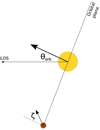 |
Fig. 1 Schematic illustration of the orbital configuration. The orbital plane is defined by the angle θorb, while the planet spins forming an obliquity angle ζ with respectto the orbital plane normal. |
2.2 Deep neural network regularized reconstruction with loop unrolling
A conceptually simple, often fast, and successful method for the solution of convex regularized problems is the iterative shrinkage thresholding algorithm (ISTA; Beck & Teboulle 2009). ISTA is a first-order proximal algorithm (Parikh & Boyd 2013) for the optimization of the following type of problems,
 (4)
(4)
where f(x) is differentiable and g(x) is a convex function. The solution is obtained by the iterative application of the steps

where ρ is a step size that needs to be properly tuned. The ISTA algorithm (and fundamentally all algorithms for the solution of regularized problems) crucially depends on the availability of a fast way to solve subproblem (6), which is known as the proximal operator. Fortunately, it is possible to find a closed form for the proximal operator for certain g(x) functions. Of special interest are the cases of ℓ1 and Tikhonov regularizations. The proximal operator for the ℓ1 regularization, where  , is given by
 (7)
(7)
where the soft thresholding (or shrinkage) operator is given by
 (8)
(8)
The proximal operator for the Tikhonov regularization, in which  , is given by
 (9)
(9)
Particularizing the ISTA method to Eq. (3), the iterative scheme is given by

where the step size ρ has an optimal value given by  , where τ is the largest eigenvalue of the ΦTΦ matrix.
We propose solving the regularized problem by leveraging deep neural networks to impose the regularization. Instead of explicitly defining the regularization function R(m), we directly model its effect as a proximal projection with the aid of a neural network, so we substitute Eq. (11) by
 (12)
(12)
where the F(k)(x) are mappings defined by convolutional neural networks whose architecture we discuss below. The F(k) (x) operators can then be seen as learned denoisers that generalize the concept of a proximal projection operator (e.g., Venkatakrishnan et al. 2013; Zhang & Ghanem 2018; Wang et al. 2019). Such iterative methods are commonly known as plug-and-play methods.
We follow Gregor & LeCun (2010) and unroll N iterations ofEqs. (10) and (12) as a deep neural network and train the networkend-to-end. The loop unrolling also allows us to learn the optimal values for ρ used in the ISTA iteration. We also allow them to be different at all iterations, unlike ISTA where they are kept constant. For clarity, we repeat here the two steps that need to be iterated for k = 1, …, N, starting from an initial solution m(0) = 0:

The learned quantities are forced to fulfill ρ(k) ~ 1 and are used to allow our trained unrolled scheme to use step sizes different from the optimal one given by ρ. We have found that the chosen initial solution gives stable reconstructions, although we can also use other potentially interesting options like m(0) = ΦTd.
The general structure of the unrolled deep network is displayed in Fig. 2. The inputs to the network are the vector of observations d and the initial solution m(0). These vectors are then used to compute r(k), which is then transformed by the nonlinear neural network to finally produce a new estimated solution. This process is iterated N times. The detail of the neural networks is shown as an inset in Fig. 2. The specifics of these networks is discussed in the following.
2.3 Denoisers
Several options are available for the layers inside the F operators. The first obvious option is to use a fully connected layer to map the HEALPix pixelization, seen as a 1D vector, to intermediate representations. We quickly discarded this option because the number of free parameters of the network increases very quickly withthe number of pixels in the sphere. The second option is to use convolutional layers, which are very efficient in the number of parameters. Our first option is what we term a 1D regularizer, which uses convolutional layers acting on the HEALPix pixelization seen as a 1D vector. This option does not exploit any specific spatial correlation on the surface of the exoplanet. As indicated in Fig. 2, we utilize four 1D convolutional layers with kernels of size 3 producing the sequence (1, Ns) → (32, Ns) → (32, Ns) → (32, Ns) → (1, Ns), where the first index indicates the number of channels and the second index indicates the number of pixels on the surface. We unroll N = 15 iterations, with a total number of ~95k free parameters. An arguably more appropriate option, which we term a 2D regularizer, is to use convolutional layers defined on the surface of the sphere using the HEALPix pixelization. We take advantage of the idea developed by Krachmalnicoff & Tomasi (2019). This option has the interesting property of exploiting the spatial information on the sphere to produce an intermediate representation. In this case we also use 32 kernels of size 3 × 3 in the intermediate layers, resulting in a total of 285k free parameters. We caution that the solution of Krachmalnicoff & Tomasi (2019) for implementing convolutions on the sphere is arguably not optimal as it produces artifacts that we discuss in the following sections. It is worth exploring other options for convolutions in the sphere (e.g., Perraudin et al. 2019).
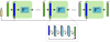 |
Fig. 2 Architecture of the deep neural network that carries out the unrolled iterative reconstruction for N steps. Each green phase plate defines the application of Eqs. (25) and (27). The internal structure of the F operator is shown in the inset. These operators are made of a train of convolutional layers with ReLU activation functions that generate Nf channels. The last layer is followed by a ReLU activation function and another linear layer. |
2.4 Tikhonov regularization
For comparison with our results we consider the Tikhonov-regularized case. We solve it using ISTA with the corresponding proximal projection operator, given by Eq. (9):

starting from m(0) = 0.
3 Mapping cloudy planets
Mapping cloudy planets is a much more challenging problem than mapping cloudless planets. If an exoplanet is similar to the Earth, one can potentially find persistent clouds that always occur in the same position on the surface together with nonpersistent clouds that form or move across the surface (e.g., Pallé et al. 2008). Persistent clouds can hardly be distinguished from the surface albedo, but nonpersistent clouds make the recovery of the surface much more difficult. Our aim here is to show that this mapping can be carried out even when using single-passband observations, although the mapping can potentially improve if multi-band observations are considered.
We consider two models for the resulting albedo in a planet with clouds. For the first we assume, for a discretized element on the surface of the planet, that ms is the surface albedo, while mc is the cloud albedo. We make the assumption that the clouds are kept stationary during a single epoch of observations to reduce the dimensionality of the solution space. We also make the assumption that clouds have a fairly low absorption in the visible while scattering is dominant. If the stellar illumination arriving at the atmosphere of the planet is F0, the amount of light reflected by the cloudwould be F0mc. A fraction F0(1 − mc) would pass downward and reflect off the planetary surface. The amount of reflected light would then be F0 (1 − mc)ms. On its return upward, a fraction mc is again dispersed and a fraction (1 − mc) would pass to the external layers of the atmosphere. Therefore, from this amount of light that comes out again, we can infer the final albedo of the planet, which is  . By plugging this expression into Eq. (1) for all surface elements, we end up with the following generative model for the observed flux at epoch i from a total of Ne epochs
 (17)
(17)
where ⊙ is the Hadamard (or elementwise) product. We note that the problem is still linear in the albedo of the planetary surface if the cloud albedo is known. On the other hand, the problem is already nonlinear in the cloud albedo. We note that ms is common to all epochs and plays the role of m in the cloudless planet. A direct application of Eqs. (5) and (6) results in the iterative scheme

where
![Mathematical equation: \begin{align*} &{\vec t}_{0;i} \,{=}\,1-{\vec m}_{\textrm{c};i}^{(k-1)},\\ &{\vec t}_{1;i} \,{=}\,{\vec t}_{0;i} \odot {\vec t}_{0;i},\\ &{\vec t}_{2;i} \,{=}\,\boldsymbol{\Phi}_i^T \left[ \boldsymbol{\Phi}_i \left({\vec m}_{\textrm{c};i}^{(k-1)} + {\vec t}_{1;i} \odot {\vec m}_{\textrm{s}}^{(k-1)} \right) - {\vec d} \right]. \end{align*}](/articles/aa/full_html/2021/02/aa40066-20/aa40066-20-eq23.png)
The F(k) operators are trained by unrolling the previous iterative scheme N times and dealing with them as an end-to-end neural network, as before.
A second slightly less complex model can also be considered. In this model we assume that the intrinsic albedo of the clouds is fixed to a value Ac. The clouds are then characterized by the coverage filling factor mc;i inside each discrete pixel on the surface of the planet at each epoch. Under this approximation the observed light curve is given by
 (24)
(24)
In this case the iterative scheme is given by

where
![Mathematical equation: \begin{align*} {\vec t}_{i} &\,{=}\,\boldsymbol{\Phi}_i^T \left[ \boldsymbol{\Phi}_i \left({\vec m}_{\textrm{s}}^{(k-1)} + (A_{\textrm{c}} - {\vec m}_{\textrm{s}}^{(k-1)}) \odot {\vec m}_{\textrm{c};i}^{(k-1)} \right) - {\vec d} \right]. \end{align*}](/articles/aa/full_html/2021/02/aa40066-20/aa40066-20-eq26.png) (28)
(28)
All results shown in this paper are obtained with the first model, but we describe the second one here for future reference.
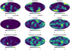 |
Fig. 3 Samples of mock planetary (upper row) and cloud (middle row) albedo surfaces that are part of the training set. The combination of the two is shown in the lower row. |
4 Training
4.1 Training dataset
The neural network is trained with simulated light curves of exoplanets in many different configurations. The main ingredients that we need to simulate are the Φ matrices, which only depend on the geometry of the problem, and the surface ms and cloud albedos mc, which changes from planet to planet. The training set is then formed by the triplet (m, d, Φ) for each example in the training database for cloudless planets. Likewise, for cloudy planets we have the quadruple (ms, mc, d, Φ) considering all observed epochs in which the cloud coverage changes.
For the definition of the planetary surface and cloud albedos we use the HEALPix pixelization, which has some desirable properties (e.g., equal area pixels, efficient available software) and has become a standard for the pixelization of the sphere, especially in astrophysics (e.g., Planck Collaboration I 2020). For this work we fix Nside = 16, which results in 3072 pixels on the surface of the planet.
Geometric kernels are used by our neural approach consistently following the ISTA iterative scheme so that they do not need to be learned by the neural network. Therefore, we can get very good generalizations to arbitrary geometries by only simulating a sufficient amount of possible geometries and obsering epochs in the training set. More crucial is the process for the generation of the surface albedos. This is precisely the information that is exploited by the neural network to denoise each step of the iterative scheme and project the solution on the set of compatible solutions.
We simulate 5000 different Φ matrices by randomly setting the rotational period from 10 to 50 days, the orbital period from 100 to 500 days, and the obliquity and inclination of the orbit from 0 to π∕2. The parameters ϕrot = ϕorb = π are kept fixed given their arbitrary character. Although varying them in suitable ranges to cover a good variety of potential Φ matrices should be considered, we think that our simulation covers a good amount of potential planet candidates observations. Additionally, a full description of the Φ matrix requires the definition of the specific observing times of each epoch. We assume we observe the planet in five epochs that are fixed as multiples of the rotation period, in particular 30, 60, 150, 210, 250. Each epoch consists of observations in steps of 1 h during an observing period of 24 h. During this 24-h interval, global clouds maps are fixed to their daily mean. All Φ matrices arecomputed with the exocartographer software package (Farr et al. 2018), using the HEALPix pixelization.
The generation of mock exoplanet surfaces is crucial for the success of the algorithm. The neural network will produce overly simple albedo surfaces if it is fed with simple surfaces. Therefore, we need to generate sufficiently complex mock albedo surfaces that can look like potential exo-Earths. One option is to use the Gaussian process generation from Farr et al. (2018). However, inspired by the computer graphics procedural generation of planetary surfaces, we prefer to use 3D Perlin noise (Perlin 1985). We use the open source libnoise library3 that generates correlated noise on the surface of the sphere to produce a database of mock procedurally generated planetary surface and cloud albedos. Three examples of the generated surface and cloud albedos are shown in Fig. 3, together with the final albedo computed with Eq. (17). We generate 5000 pairs of mock albedo surfaces and clouds for the training by modifying the seed of the Perlin noise generator. The surface albedo contains large zones of low albedo which can be compatible with oceans.
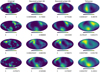 |
Fig. 4 Neural and Tikhonov reconstructions of four different mock cloudless planets observed at the same five epochs as those in the training set. In this case, all of them share Prot = 24 h, Porb = 365 days, θorb = 0°, and ζ = 90°. Shown are the reconstructions carried out with 1D and 2D convolutional networks. |
4.2 Training the neural network
The training proceeds by chunking the training set in batches of size Nb = 128 cases for the denoiser that uses 1D convolutions, and Nb = 32 for the denoiser that uses 2D convolutions in the sphere (the reduction in the batch size comes from limitations in the GPU memory). These batches are then fed to the unrolled neural network in sequence. For each batch our aim is to force the discrepancy between the reconstructed albedo map and that of the training set to be as small as possible. The loss function to be minimized is
 (29)
(29)
We note that we force all phases of the unrolled neural network to produce intermediate solutions that get close to the albedo map in the training set (with weight ωk, which we set to ωk = 1), instead of just the final output, m(N). We found that this produced a slightly faster behavior during training. The learnable parameter set includes the weights of all the convolutional layers of F and the step sizes ρ(k). We additionally force ρ(k) to be in the interval [0.1, 3].
We define and train the unrolled deep neural network in PyTorch 1.6 (Paszke et al. 2019), which can efficiently compute the gradient of the loss with respect to the parameters using automatic differentiation. We use the Adam stochastic gradient optimizer (Kingma & Ba 2014) with a learning rate of 3 × 10⁻⁴ during 50 epochs. We found that the chosen learning rate produces suitable results and it was kept fixed for all experiments. During training, Nb geometrical kernels and albedo surfaces are randomly picked up from the available database to construct each batch. A total of 20k simulated light curves are used in each epoch of the training. We utilize an NVIDIA RTX 2080 Ti GPU for the computations; the computing time per epoch during training is ~60 s in the case of 1D convolutions and ~11 min in the case of 2D convolutions. A set of unseen validation examples is also reconstructed with the network at the end of each epoch to check for overfitting. At the end of training we freeze the neural network parameters that produces the smallest loss function in the validation set in order to produce the results shown in the next section.
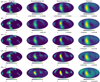 |
Fig. 5 Noise sensitivity of the reconstruction of a mock planet. The geometric parameters are the same as those in Fig. 4 and the signal-to-noise ratio of the light curve is shown in each case. |
5 Results
5.1 Cloudless mock planets
We start by analyzing the results when new mock albedo surfaces are used using the two options that we consider for the denoising operators: 1D or 2D convolutions in the sphere. Although having fast reconstructions is not a real issue at the moment, we note that the reconstruction of a map with 3072 pixels can be done in ~6 ms when using 1D convolutionsand in ~11 ms when using 2D convolutions. These reconstruction times are obtained by making use of the GPU, and do not take into account any memory transfer time between the main memory and that of the GPU or viceversa, which is often a limiting factor. The quoted times include the application of the N = 15 unrolled steps, together with the application of the denoising neural networks in each step. Although we impose the loss function over all steps of the unrolled iterative scheme, the results we show are those obtained in the last step.
The reconstruction of four mock planets are displayed in Fig. 4. The parameters are Prot = 24 h, Porb = 365 days, θorb = 0°, and ζ = 90°. This corresponds to a face-on observation of the star–planet system, with the planet spinning axis contained in the ecliptic plane. This configuration, although probably not dynamically stable, allows us to see the planet continuously spinning, while the illuminated hemisphere changes during the orbital period. We chose this configuration also for easy comparison with previous works that made use of it (e.g., Kawahara & Fujii 2011; Kawahara & Masuda 2020). The planet is observed at the same five epochs used during training, which turns out to be a very sparse sampling of the light curve. The noise injected on the light curve is such that we end up with a S∕N = 2.3. The left column shows the original map, the middle columns shows the two neural reconstructed albedo maps, and the last column displays the map inferred with the Tikhonov regularization with λ = 0.5 and using the optimal value of ρ. The value ofλ was found by trial-and-error looking for the most contrasted reconstruction without visible artifacts. Both neural reconstructions show a quite remarkable resemblance with the original map except for some of the high spatial frequency variations. We note that the artifactsin the 1D regularizer comes from not imposing any spatial coherence during the regularization. One of the most conspicuous artifacts is a checkerboard structure that disappears when using the 2D regularizer. All our experiments suggest that the 2D regularizer should be taken as the baseline.
The neural reconstruction produces much more compact large albedo regions, in closer agreement with the original maps. However, both reconstructions are unable to reach the amplitude of the largest albedo regions. Likewise, the very low or zero albedo regions in the original map are reconstructed with slightly larger albedos, which are used to compensate for the large albedo regions. It is clear that the neural reconstruction leads to a much better representation of the albedo map than the Tikhonov-regularized case. Interestingly, we find no visible artifacts on the reconstruction in the poles, even though the observational configuration has no access to them.
The neural reconstruction is very resilient to the presence of noise in the light curve, as shown in Fig. 5 for a single mock surface. The geometric parameters are kept fixed and equal to those in Fig. 4. Increasingly larger amounts of noise are injected into the observed light curve, giving rise to a broad variation in the S/N, from 0.2 to 23. The value of the regularization parameter in the Tikhonov reconstructions has been optimized, by trial-and-error, to produce the best result possible. It is obvious that the Tikhonov regularization struggles to reconstruct the low albedo regions when the noise is very large, while the neural approach consistently recovers a very robust map, even for very low S/N. When the S/N is very low, the neural and Tikhonov reconstructions both display regions with large albedos that were not present in the original surface.
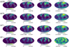 |
Fig. 6 Reconstruction of the cloudless Earth at different S/N. The parameter σ refers to thestandard deviation of the noise added to the light curve. The coastlines are shown for reference. |
5.2 Cloudless Earth
As an example of the reconstruction of a cloudless planet we show the reconstruction of the Earth albedo. The albedo map that we use corresponds to February 2017, obtained from the NASA Earth Observation (NEO) webpage4. We simulate the observation of the Earth for θorb = 0° and ζ = 90°. The light curve is observed for one orbital period (365.25 days) with a cadence of 5 h, producing a total of ~ 1750 points in the light curve. We assume that the observations are instantaneous, neglecting the smearing effect produced by the rotation. The two neural reconstructions displayed in Fig. 6 both produce very reliable maps of the surface albedo of the Earth. Almost all continents (North America, South America, Europe, Asia, and Africa) are clearly recovered, with their fine structure in the albedo. The high albedo of the Sahara desert, central Asia, and the northern part of North America are very well recovered even when the S∕N ~ 1, with almost the same extension as in the original surface albedo. Antarctica is not recovered properly because of the limited access to the poles in this configuration. Additionally, Australia is recovered at a different latitude.
On the contrary, the Tikhonov regularized maps show very smooth continents. The reconstruction is very robust to the presence of noise on the light curve. Even when the signal is buried in the noise, with a very low S∕N = 0.2, the reconstruction is very robust. Some details are lost and in some cases artifacts appear. However, a comparison with what is achieved with Tikhonov shows the potential for the learned regularization.
5.3 Cloudy Earth
We now turn our attention to the difficult problem of mapping cloudy planets. We analyze whether the surface of an exo-Earth and the clouds can be mapped with our neural approach. To this end, we assume that we observe the Earth during a year with a cadence of 5 h with a S∕N = 16. We use the same surface albedo that was used for the cloudless Earth mapping in Fig. 6. The Earth’s daily-averaged cloud cover maps are obtained from the daily 20-y database of the International Satellite Cloud Climatology Project5 (Rossow & Bates 2019). We arbitrarily chose to use the data from 2004. Even though the database contains a different cloud cover map each day, we make the simplifying assumption that the cloud cover is stable for one week. Since the typical lifetime of large-scale cloud pattern on Earth is about one week (Pallé et al. 2008), this constrains the problem slightly better.
We consider two observational geometries, both of which potentially allow a complete mapping of the surface. The first is a face-on observation (θorb = 0°) with obliquity ζ = 90°. This configuration, similar to that used in the previous examples, produces an illuminated hemisphere that changes smoothly with the orbit from the north pole to the south pole and vice versa, while the spinning modulation gives information about the structures in the illuminated hemisphere. The second case is an edge-on configuration (θorb = 90°) with obliquity ζ = 23° without considering the eclipse. This configuration is less informative because the observations are much more sensitive to the equatorial and tropical regions than to those of higher latitudes, but it is a much more likely scenario for real exoplanet observations.
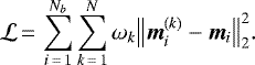
Figure 7 shows the results of applying the neural reconstruction using the two denoisers. The upper row displays the original map, the two reconstructed maps, and the weight that this configuration puts on every point on the surface. The remaining rows display the original cloud albedo (rows 1 and 3) and the inferred cloud albedo (rows 2 and 4) for eight epochs along the year of observation (labeled with the specific week). When compared with Fig. 6, the inferred surface albedos are strongly affected by the presence of the clouds. The high albedo of North America is correctly recovered, but the Sahara desert and Central Asia high albedo regions are slightly displaced in latitude, probably as a consequence of the persistent clouds, as explained in the following. We have checked that this displacement is reduced and the maps converge towards those of Fig. 6 when the amount of clouds is reduced.
The cloud albedo on each epoch clearly shows the partial information produced by the change in the illuminated hemisphere. We note that the amplitude of the inferred albedo of the clouds is systematically very low. This is probably a consequence of the weak dependence of the total albedo on the specific albedo of the clouds when the surface albedo is high. For this reason, although the learned scheme tends to produce low albedos for the clouds, it is possible to scale them up while still fitting the observations. As a consequence, obtaining absolute cloud albedos does not seem to be possible with monochromatic observations.
Even if we cannot obtain the cloud map per epoch, it is worth analyzing if we can recover the mean cloud coverage and, more interestingly, a measure of its variability. The upper row of Fig. 8 shows the 2004 yearly-mean cloud coverage for Earth and its relative variability (defined as the standard deviation normalized by the mean). The most conspicuous features are persistent clouds close to the east coast of South America; in the northern part of America, Europe, and Asia; and in the southern coast of Australia. These are in good agreement with some of the regions of high albedo obtained in the neural reconstructions. Therefore, we conclude that these reconstructions are able to obtain a combination of the surface albedo, together with the persistent clouds. Additionally, the recovered cloud relative variability (lower row) nicely correlates with that measured on Earth. Large cloud relative variabilities are found close to the Equator, in southern Africa, and in part of eastern Asia. These are areas with strong daily and seasonal cloud variability. Consequently, we conclude that this mapping method is able to obtain a rough estimate of cloud variability on an exo-Earth. When applied to rocky planets in the habitable zone of their host stars, the bulk atmospheric composition from spectroscopic studies as well as the measured equilibrium temperature of the planet will be able to constrain and associate this cloud variability with that of the water cycle, implying not only water vapor in the planetary atmosphere, but also significant amounts of liquid water in the surface.
Finally, we show in Fig. 9 the reconstructions in the edge-on observation. Unfortunately, the limited latitude sensitivity of this configuration introduces an ambiguity in latitude of all structures that cannot be overcome. Even so, the recovered D-shaped maps capture well the three major continental features of the original maps (Americas, Europe/Africa, and Asia), and thus the inhomogeneity of the planet’s surface. We have been unable to significantly improve the quality of the mapping by increasing the duration of the light curve. As a consequence of the poor mapping of the surface, the cloud mapping is also defective and the cloud variability is also poorly inferred.
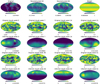 |
Fig. 7 Reconstruction of a cloudy exo-Earth when observed face-on, with θorb = 0° and ζ = 90°. Top row: original surface albedo map, together with the two reconstructions using different denoisers, as well as the relative weight for each element on the surface. The next pairs of rows display the original cloud coverage (rows 2 and 4), togetherwith the inferred cloud albedo (rows 3 and 5). |
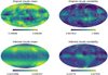 |
Fig. 8 Mean cloud cover on Earth in 2004 (top left) and maps of its variability (top right). Bottom panels: same recovered maps for a simulated Earth, when observed face-on, with θorb = 0° and ζ = 90°. |
6 Conclusions
We presented a mapping technique for exo-Earths using neural networks as regularizers6. The standard iterative scheme for the solution of linear problems with regularization is unrolled as a neural network and trained in an end-to-end fashion. The best regularizer is found to be a convolutional neural network acting on the surface of the planet. Given the absence of observed maps of exo-Earths, we used albedo surfaces generated procedurally to mimick our planet. The mapping technique is general and can be re-trained in case better options for albedo surfaces are found in the future.
We apply the method to cloudless planets, showing that the surface of such planets can be very well recovered with our methodology. The position of the continents and their extension shows a clear improvement with respect to more standard regularizations like Tikhonov. Additionally, the results are extremely resilient to the presence of noise on the light curve. We also show how cloudy planets can also be roughly mapped with the same method using only monochromatic observations. The inferred albedo maps contain information about a combination of the surface albedo and persistent clouds, which cannot be disentangled. This degeneracy can potentially be broken if polychromatic observations are used if clouds and surface albedos have a different behavior with wavelength (Cowan et al. 2009).
Finally, although detailed cloud mapping for each observing epoch cannot be accurately retrieved, we show that we can obtain a good estimation of the mean persistent cloud distribution and, more importantly, their map of variability. If applied to rocky planets in the habitable zone of their stars, this cloud variability map, together with the measured bulk atmospheric composition and equilibrium temperature of the planet, will be able to constrain the presence of a water cycle in the planetary atmosphere or on the surface. Thus, our method implies the potential to empirically infer the presence of significant amounts of liquid water on the planet’s surface.
Acknowledgements
We acknowledge financial support from the Spanish Ministerio de Ciencia, Innovación y Universidades through project PGC2018-102108-B-I00 and FEDER funds. This research has made use of NASA’s Astrophysics Data System Bibliographic Services. We acknowledge the community effort devoted to the development of the following open-source packages that were used in this work: numpy (numpy.org, Harris et al. 2020), matplotlib (matplotlib.org, Hunter 2007), PyTorch (pytorch.org, Paszke et al. 2019) and zarr (github.com/zarr-developers/zarr-python).
References
- Aizawa, M., Kawahara, H., & Fan, S. 2020, ApJ, 896, 22 [CrossRef] [Google Scholar]
- Beck, A., & Teboulle, M. 2009, SIAM J. Imag. Sci., 2, 183 [CrossRef] [Google Scholar]
- Berdyugina, S. V., & Kuhn, J. R. 2019, AJ, 158, 246 [CrossRef] [Google Scholar]
- Candès, E. J., Romberg, J. K., & Tao, T. 2006, Commun. Pure Appl. Math., 59, 1207 [CrossRef] [MathSciNet] [Google Scholar]
- Cowan, N. B., Agol, E., Meadows, V. S., et al. 2009, ApJ, 700, 915 [NASA ADS] [CrossRef] [Google Scholar]
- Des Marais, D. J., Harwit, M. O., Jucks, K. W., et al. 2002, Astrobiology, 2, 153 [NASA ADS] [CrossRef] [PubMed] [Google Scholar]
- Farr, B., Farr, W. M., Cowan, N. B., Haggard, H. M., & Robinson, T. 2018, AJ, 156, 146 [CrossRef] [Google Scholar]
- Ford, E. B., Seager, S., & Turner, E. L. 2001, Nature, 412, 885 [NASA ADS] [CrossRef] [PubMed] [Google Scholar]
- Fujii, Y., & Kawahara, H. 2012, ApJ, 755, 101 [NASA ADS] [CrossRef] [Google Scholar]
- Goodfellow, I., Bengio, Y., & Courville, A. 2016, Deep Learning (Cambridge: MIT Press) [Google Scholar]
- Gregor, K., & LeCun, Y. 2010, Proc. International Conference on Machine learning (ICML’10), 399 [Google Scholar]
- Hardegree-Ullman, K. K., Cushing, M. C., Muirhead, P. S., & Christiansen, J. L. 2019, AJ, 158, 75 [NASA ADS] [CrossRef] [Google Scholar]
- Harris, C. R., Millman, K. J., van der Walt, S. J., et al. 2020, Nature, 585, 357 [CrossRef] [PubMed] [Google Scholar]
- Hunter, J. D. 2007, Comput. Sci. Eng., 9, 90 [NASA ADS] [CrossRef] [Google Scholar]
- Kawahara, H. 2020, ApJ, 894, 58 [CrossRef] [Google Scholar]
- Kawahara, H., & Fujii, Y. 2010, ApJ, 720, 1333 [CrossRef] [Google Scholar]
- Kawahara, H., & Fujii, Y. 2011, ApJ, 739, L62 [CrossRef] [Google Scholar]
- Kawahara, H., & Masuda, K. 2020, ApJ, 900, 48 [CrossRef] [Google Scholar]
- Kingma, D. P., & Ba, J. 2014, CoRR, abs/1412.6980 [Google Scholar]
- Krachmalnicoff, N., & Tomasi, M. 2019, A&A, 628, A129 [CrossRef] [EDP Sciences] [Google Scholar]
- Léger, A., Mariotti, J. M., Mennesson, B., et al. 1996, Icarus, 123, 249 [NASA ADS] [CrossRef] [Google Scholar]
- Luger, R., & Barnes, R. 2015, Astrobiology, 15, 119 [NASA ADS] [CrossRef] [Google Scholar]
- Luger, R., Agol, E., Foreman-Mackey, D., et al. 2019a, AJ, 157, 64 [NASA ADS] [CrossRef] [Google Scholar]
- Luger, R., Bedell, M., Vanderspek, R., & Burke, C. J. 2019b, AAS J., submitted [Google Scholar]
- Meadows, V. S., Reinhard, C. T., Arney, G. N., et al. 2018, Astrobiology, 18, 630 [CrossRef] [Google Scholar]
- Pallé, E., Ford, E. B., Seager, S., Montañés-Rodríguez, P., & Vazquez, M. 2008, ApJ, 676, 1319 [NASA ADS] [CrossRef] [Google Scholar]
- Pallé, E., Zapatero Osorio, M. R., Barrena, R., Montañés-Rodríguez, P., & Martín, E. L. 2009, Nature, 459, 814 [NASA ADS] [CrossRef] [PubMed] [Google Scholar]
- Pallé, E., Zapatero Osorio, M. R., & García Muñoz, A. 2011, ApJ, 728, 19 [NASA ADS] [CrossRef] [Google Scholar]
- Parikh, N., & Boyd, S. 2013, Proximal Algorithms, Foundations and Trends in Optimization (Boston: Now Publishers) [Google Scholar]
- Paszke, A., Gross, S., Massa, F., et al. 2019, in Advances in Neural Information Processing Systems 32, eds. H. Wallach, H. Larochelle, A. Beygelzimer, et al. (New York: Curran Associates, Inc.), 8024 [Google Scholar]
- Perlin, K. 1985, Proceedings of the 12th Annual Conference on Computer Graphics and Interactive Techniques, SIGGRAPH ’85 (New York, NY, USA: Association for Computing Machinery), 287 [CrossRef] [Google Scholar]
- Perraudin, N., Defferrard, M., Kacprzak, T., & Sgier, R. 2019, Astron. Comput., 27, 130 [NASA ADS] [CrossRef] [Google Scholar]
- Planck Collaboration I. 2020, A&A, 641, A1 [CrossRef] [EDP Sciences] [Google Scholar]
- Rossow, W. B., & Bates, J. J. 2019, Bull. Am. Meteorol. Soc., 100, 2423 [CrossRef] [Google Scholar]
- Snellen, I. A. G., de Kok, R. J., le Poole, R., Brogi, M., & Birkby, J. 2013, ApJ, 764, 182 [NASA ADS] [CrossRef] [Google Scholar]
- Tarter, J. C., Backus, P. R., Mancinelli, R. L., et al. 2007, Astrobiology, 7, 30 [NASA ADS] [CrossRef] [PubMed] [Google Scholar]
- Venkatakrishnan, S. V., Bouman, C. A., & Wohlberg, B. 2013, 2013 IEEE Global Conference on Signal and Information Processing, 945 [CrossRef] [Google Scholar]
- Wang, L., Sun,C., Fu, Y., Kim, M. H., & Huang, H. 2019, 2019 IEEE/CVF Conference on Computer Vision and Pattern Recognition (CVPR), 8024 [CrossRef] [Google Scholar]
- Zhang, J., & Ghanem, B. 2018, in Proceedings of the IEEE conference on computer vision and pattern recognition, 1828 [Google Scholar]
The ℓ1 norm of a vector is given by  .
.
All Figures
|
Fig. 1 Schematic illustration of the orbital configuration. The orbital plane is defined by the angle θorb, while the planet spins forming an obliquity angle ζ with respectto the orbital plane normal. |
| In the text | |
|
Fig. 2 Architecture of the deep neural network that carries out the unrolled iterative reconstruction for N steps. Each green phase plate defines the application of Eqs. (25) and (27). The internal structure of the F operator is shown in the inset. These operators are made of a train of convolutional layers with ReLU activation functions that generate Nf channels. The last layer is followed by a ReLU activation function and another linear layer. |
| In the text | |
|
Fig. 3 Samples of mock planetary (upper row) and cloud (middle row) albedo surfaces that are part of the training set. The combination of the two is shown in the lower row. |
| In the text | |
|
Fig. 4 Neural and Tikhonov reconstructions of four different mock cloudless planets observed at the same five epochs as those in the training set. In this case, all of them share Prot = 24 h, Porb = 365 days, θorb = 0°, and ζ = 90°. Shown are the reconstructions carried out with 1D and 2D convolutional networks. |
| In the text | |
|
Fig. 5 Noise sensitivity of the reconstruction of a mock planet. The geometric parameters are the same as those in Fig. 4 and the signal-to-noise ratio of the light curve is shown in each case. |
| In the text | |
|
Fig. 6 Reconstruction of the cloudless Earth at different S/N. The parameter σ refers to thestandard deviation of the noise added to the light curve. The coastlines are shown for reference. |
| In the text | |
|
Fig. 7 Reconstruction of a cloudy exo-Earth when observed face-on, with θorb = 0° and ζ = 90°. Top row: original surface albedo map, together with the two reconstructions using different denoisers, as well as the relative weight for each element on the surface. The next pairs of rows display the original cloud coverage (rows 2 and 4), togetherwith the inferred cloud albedo (rows 3 and 5). |
| In the text | |
|
Fig. 8 Mean cloud cover on Earth in 2004 (top left) and maps of its variability (top right). Bottom panels: same recovered maps for a simulated Earth, when observed face-on, with θorb = 0° and ζ = 90°. |
| In the text | |
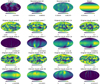 |
Fig. 9 Same as Fig. 7, but for edge-on observation with θorb = 90° and ζ = 23°. |
| In the text | |
Current usage metrics show cumulative count of Article Views (full-text article views including HTML views, PDF and ePub downloads, according to the available data) and Abstracts Views on Vision4Press platform.
Data correspond to usage on the plateform after 2015. The current usage metrics is available 48-96 hours after online publication and is updated daily on week days.
Initial download of the metrics may take a while.