| Issue |
A&A
Volume 664, August 2022
|
|
|---|---|---|
| Article Number | A59 | |
| Number of page(s) | 21 | |
| Section | Planets and planetary systems | |
| DOI | https://doi.org/10.1051/0004-6361/202142932 | |
| Published online | 09 August 2022 | |
Exoplanet cartography using convolutional neural networks
1
Faculty of Aerospace Engineering, Delft University of Technology,
Kluyverweg 1,
2629
HS Delft, The Netherlands
2
Delft Institute of Applied Mathematics, Delft University of Technology,
Mekelweg 4,
2628
CD Delft, The Netherlands
e-mail: p.m.visser@tudelft.nl
Received:
16
December
2021
Accepted:
25
April
2022
Context. In the near future, dedicated telescopes will observe Earth-like exoplanets in reflected parent starlight, allowing their physical characterization. Because of the huge distances, every exoplanet will remain an unresolved, single pixel, but temporal variations in the pixel’s spectral flux contain information about the planet’s surface and atmosphere.
Aims. We tested convolutional neural networks for retrieving a planet’s rotation axis, surface, and cloud map from simulated single-pixel observations of flux and polarization light curves. We investigated the influence of assuming that the reflection by the planets is Lambertian in the retrieval while in reality their reflection is bidirectional, and the influence of including polarization.
Methods. We simulated observations along a planet’s orbit using a radiative transfer algorithm that includes polarization and bidirectional reflection by vegetation, deserts, oceans, water clouds, and Rayleigh scattering in six spectral bands from 400 to 800 nm, at various levels of photon noise. The surface types and cloud patterns of the facets covering a model planet are based on probability distributions. Our networks were trained with simulated observations of millions of planets before retrieving maps of test planets.
Results. The neural networks can constrain rotation axes with a mean squared error (MSE) as small as 0.0097, depending on the orbital inclination. On a bidirectionally reflecting planet, 92% of ocean facets and 85% of vegetation, deserts, and cloud facets are correctly retrieved, in the absence of noise. With realistic amounts of noise, it should still be possible to retrieve the main map features with a dedicated telescope. Except for face-on orbits, a network trained with Lambertian reflecting planets yields significant retrieval errors when given observations of bidirectionally reflecting planets, in particular, brightness artifacts around a planet’s pole. Including polarization improves the retrieval of the rotation axis and the accuracy of the retrieval of ocean and cloudy map facets.
Key words: planets and satellites: surfaces / planets and satellites: oceans / planets and satellites: atmospheres / techniques: photometric / techniques: polarimetric / techniques: image processing
© K. Meinke et al. 2022
 Open Access article, published by EDP Sciences, under the terms of the Creative Commons Attribution License (https://creativecommons.org/licenses/by/4.0), which permits unrestricted use, distribution, and reproduction in any medium, provided the original work is properly cited.
This article is published in open access under the Subscribe-to-Open model. Subscribe to A&A to support open access publication.
1 Introduction
Since the discovery of the first exoplanet by Mayor & Queloz (1995), more than 4000 exoplanets have been identified and cataloged.1 Statistically, nearly every star has exoplanets (Bryson et al. 2020; Dressing & Charbonneau 2015; Tuomi et al. 2014), and several of these will be rocky and in the habitable zone of their star, where the ambient conditions could allow the presence of liquid water. In particular, Earth-like landscapes with continents and shallow water regions between water oceans appear to be a promising environment for life to form and evolve. With the aim of finding potentially habitable exoplanets and traces of extraterrestrial life, scientists are thinking about designing and optimizing the next generation of space and ground-based telescopes and instruments that would be able to characterize small, rocky exoplanets in the habitable zones of their stars (see for example, the recently published “Pathways to Discovery in Astronomy and Astrophysics for the 2020s” by the National Academies of Sciences, Engineering, and Medicine 2021).
The techniques that are currently the most successful in detecting such small, rocky exoplanets are the transit method and the radial velocity method, which give little information about the planet’s characteristics besides the (minimum) mass and the orbital parameters. The latter allows one to compute the amount of incoming stellar flux and estimate, albeit very roughly, the average surface temperature and the possible presence of liquid water on the planet and hence the possible presence of liquid surface water, if the planet is of the terrestrial type.
A future technique to characterize the physical properties of small planets is the direct detection of light that these planets reflect as they orbit their parent star. This is very difficult because these planets are extremely faint compared to their parent star; the star will usually be at least 10 million times brighter than the planet (see Hunziker et al. 2020; Snellen et al. 2021, and references therein). The most promising candidates for direct observations of Earth-like exoplanets orbiting solar-type stars are space telescopes, in particular when flown in combination with a starshade. This architecture was originally proposed by Cash (2006) and it makes use of a starshade spacecraft that blocks out the star’s bright light, allowing a distant, formation flying space telescope to directly observe the reflected starlight of the orbiting planets. Two starshade missions have been selected for study: the Starshade Rendezvous Probe that aims to add a starshade to the Nancy Grace Roman Space Telescope (Seager & Kasdin 2018) (to be launched before 2030), and the HabEx mission (JPL 2019) that consists of a space telescope and a dedicated starshade (to be launched in the mid-2030s). The next generation of ground-based telescopes, such as the Extremely Large Telescope (ELT)2 will also have the capability to directly image Earth-like exoplanets around nearby M-type stars, but the contrast needed to detect signals of such planets around Sun-like stars appears to be hard to achieve.
Apart from measuring the total flux of light that is reflected by an exoplanet, some telescope designs also aim to measure the degree and direction of linear polarization of this light, for example, the Nancy Grace Roman Space Telescope (Maier et al. 2021), and it is being considered for HabEx and LUVOIR (a UV-space telescope concept) (see Snellen et al. 2021, and references therein). Polarimetry for the characterization of small exoplanets, in particular the detection of oceans, was explicitly mentioned in “Pathways to Discovery in Astronomy and Astrophysics for the 2020s” (National Academies of Sciences, Engineering, and Medicine 2021).
Dedicated space and/or ground-based telescopes, with or without polarimetric capabilities, are expected to take the first images of Earth-like exoplanets sometime in the next decades. However, due to the huge distances, these exoplanets will appear as single pixels in any such image, much like the Earth itself in the iconic Pale Blue Dot picture taken from about 6 billion kilometers distance by Voyager 1.
Even with the largest telescope concepts, the photons received from a small exoplanet will have to be collected for up to hours to make sure that the planet signal rises above the noise. In Fig. 1, we show the number of photons that would be received by the Starshade Rendezvous Probe (with the Nancy Grace Roman Space Telescope) and HabEx, which have apertures of 2.4 and 4 m, respectively, for a completely white, Earth-sized planet around a solar-type star at full phase (the planet is then actually behind the star, so this is a theoretical maximum value). We furthermore assumed that the total flux in a 50 nm-wide spectral band is integrated over 3 h.
If the planet’s surface is horizontally inhomogeneous and/or if the planet has a broken cloud-deck, its total flux signal as well as its polarization signal will vary as the planet rotates about its axis and different parts of its surface are illuminated by the light of its parent star. The planet’s signal will thus depend on the longitudinal variation over the planet. Also, as the planet orbits the star, its phase will change, just like the lunar phase changes throughout a month. With an exoplanet, we will, however, not see a change in the shape of the illuminated disk, as we do for the Moon, but a change in the overall total and polarized fluxes of the unresolved pixel. As can be seen in Fig. 2, the range of phase angles that the planet will cover along its orbit depends on the inclination angle i of the orbit: if the orbit is seen edge-on (i = 90°), the phase angle α varies between almost 0° to 180°, while if the orbit is face-on (i = 0°), the phase angle is always 90°. From which part of the exoplanet an observer will receive reflected starlight at any given phase angle also depends on the orientation of the rotation axis of the planet. If the axis is tilted with respect to the planet’s orbital plane, the substellar point travels between the tropical circles. This results in a reflected light signal that depends on the surface and cloud variation with latitude.
Because the reflection properties of a planetary surface and atmospheric constituents will also depend on the wavelength, the reflected light signal of a rotating planet will thus depend on time and also on the wavelength, (Ford et al. 2001; Groot et al. 2020, and references in the latter). Measurements of the temporal and spectral variations of the signal of a single pixel exoplanet contain information about the horizontal variability of the planet. How to retrieve a surface map of an exoplanet from reflected total flux light curves has been studied by Fujii & Kawahara (2012); Kawahara & Masuda (2020); Fan et al. (2019); Farr et al. (2018); Asensio Ramos & Pall6 (2021). They have shown that it is indeed possible to constrain a planet’s rotation axis and retrieve a rough planetary surface map. In these studies, the planet’s surfaces are treated as Lambertian reflectors, which diffusely reflect starlight in all directions.
Lambertian reflectors do not include polarization. As the total flux of the reflected starlight depends on the properties of the illuminated and visible part of the planetary disk, so does the linear polarization signal of this light. While the starlight that is incident on the planet can be assumed to be unpolarized, Rayleigh scattering by the gases in the atmosphere, scattering by cloud particles and reflection by surfaces like oceans will usually polarize the reflected light, depending on the directions of the incident and reflected light, and hence depending on the phase angle and the location on the planet (for polarization signals of Earth-like planets, see Stam 2008; Groot et al. 2020; Trees & Stam 2019, and references therein).
Here, we propose a retrieval algorithm that uses light curves computed assuming bidirectional reflection, as described by Rossi et al. (2018) and Trees & Stam (2019). The radiative transfer computations fully include polarization and multiple scattering and are performed for an Earth-like atmosphere with Rayleigh scattering, water clouds that create a rainbow at certain phase angles and thus orbital locations (Fig. 2 shows such locations along the planetary orbits) and oceans that exhibit the bright glint pattern due to specular reflection. The glint significantly affects a planet’s bidirectional reflection curve as compared to Lambertian reflection.
The use of bidirectional and polarized light curves requires a new approach to planet mapping. Since bidirectional reflection is more complicated than Lambertian reflection, analytical methods would be difficult to apply so different tools are required. We used neural networks, which have several advantages: they are universal approximators (Hornik 1991) and can thus find a planet’s rotation axis and they have achieved state-of-the-art results in classification problems (Schmidhuber 2015), and surface mapping is at heart a classification problem. Our neural networks are designed to use the temporal variations of the reflected light signal of an exoplanet to retrieve planet characteristics such as the orientation of the rotation axis, the surface and the cloud coverage. Our networks were trained with a large set of simulated observations of various model planets before being provided with the validation data set, which are simulated observations of model planets that were not in the training set.
In Sect. 2, we describe the characteristics of our model planets including the surface types that we consider, and we explain the numerical method that we used to simulate the total and polarized flux curves of our model planets, and the model observations, including photon noise, in the training and the test data sets. In Sect. 3, we describe the general architectures of our neural networks, how they compare to other networks that have been applied in similar research questions, and how we train and validate the network. In Sects. 4, 5, and 6, we describe the specific neural network architectures and the results for the retrievals of planetary rotation axes, albedo maps, and surface type maps, respectively. In these sections, we also investigate the retrieval errors that result from training a neural network on Lambertian reflecting planets and applying it then on realistically bidirectionally reflecting test planets, and we discuss the benefits of including polarization. In Sect. 8, we provide our conclusions and a number of recommendations for future work.
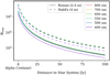 |
Fig. 1 Number of photons that would be detected by the Nancy Grace Roman and HabEX space telescopes (apertures 2.4 m and 4.0 m, respectively) from a white, Lambertian reflecting, Earth-sized planet in a 1 au orbit around a solar-type star at α = 0°, in optical spectral bands with widths of 50 nm for a 3.0 h observation. These lines can be regarded as upper bounds for the number of photons from an Earth-twin (the lines for the 500, 550, 600, 700, and 800 nm bands are very close together). The signal-to-noise ratio is proportional to |

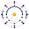 |
Fig. 2 Planetary orbits with inclination angles i ranging from 0° to 90°. The lower half of the figure is closest to the observer (we thus define i as the angle between the orbit normal and the vector to the observer). Each planetary system is defined with respect to a Cartesian coordinate system (x, y, z), with the x-axis pointing toward the observer, and the y- and z-axis as shown. Points where the planets have the same phase angle, α (defined as the angle between the vectors from the planet toward the star and the observer), form circles, because they lie on a cone with a tip-angle equal to α and also on a sphere with the radius of the (circular) orbits. The rainbow is thus a semicircle, since it is the intersection at α = 38°. The color sequence of the rainbow is reversed compared to the rainbow that forms in rain droplets (Karalidi et al. 2012). Planets are shown at the eight locations where we assume observations would be taken. |
2 Method: Radiative Transfer
2.1 Total and Polarized Fluxes
We provided our neural network with simulated observations of the total and polarized fluxes of starlight reflected by an exoplanet. These fluxes form a so-called Stokes vector (see Hansen & Travis 1974):
![$ I = \left[ {\matrix{ I \cr Q \cr U \cr V \cr } } \right], $](/articles/aa/full_html/2022/08/aa42932-21/aa42932-21-eq2.png) (1)
(1)
with I the total flux, Q and U the linearly polarized fluxes, (Q2 + U2)1/2 the total linearly polarized flux, and V the circularly polarized flux.
The reflected vector I that arrives at a distant observer pertains to the planet as a single point of light, and thus comprises the locally reflected light integrated over the illuminated and visible part of the planetary disk. Given a wavelength λ and a planetary phase angle α, vector I can be computed using (see Eq. (5) in Stam et al. 2004)
 (2)
(2)
Here, AG is the planet’s geometric albedo, which generally depends on λ through the spectral dependence of the planet’s reflective properties (for a horizontally inhomogeneous planet, this will depend on which part of the planet is facing the observer), r is the radius of the planet, and D is the distance between the planet and the observer. Furthermore, πF0 is the stellar flux incident on the planet, which we assume to be unpolarized and unidirectional. Furthermore, R is the vector describing the angular variation of the starlight reflected by the planet (this is represented by a vector instead of a matrix because we assume that the starlight is unpolarized); R depends on the characteristics of the planetary surface and atmosphere, the wavelength λ, and the illumination and viewing geometries.
Because the circularly polarized flux V of Earth-like planets is approximately 5 orders of magnitude smaller than the total flux I (see for example Groot et al. 2020), its detection is virtually impossible. We therefore ignore V in our simulations. The other vector elements are normalized such that I equals one at a phase angle of 0°, and we thus used AGI as the planet’s (flux) phase curve. Next, we describe the surface and atmosphere characteristics of our model planets.
2.2 Phase Curves for Homogeneous Planets
Similar to Earth, our model planets are covered by different surface types and have gaseous atmospheres that can contain liquid water clouds. Our radiative-transfer algorithm (Rossi et al. 2018), computes the starlight that is reflected by a locally plane-parallel and horizontally homogeneous surface-atmosphere model, where the atmosphere consists of a stack of homogeneous layers. To capture the spatial variation in surface-atmosphere models while adhering to the requirements of our radiative transfer algorithm, we describe each spherical planet with locally flat facets each of which is assigned a specific surface-atmosphere model.
We use three surface types: ocean, sandy desert, and vegetation. We do not include ice for polar caps and we limit ourselves to a static model. Although ice caps can be permanent, a realistic model would account for seasonal growing and melting depending on the obliquity of the planet’s rotation axis. Studying the retrieval of such seasonal effects is beyond the aims of this work (see the recommendations in Sect. 8).
The reflection by a given facet depends not only on the local surface-atmosphere model and wavelength λ, but also on the local zenith angle of the star, the local zenith angle of the observer, and the azimuthal angle between the directions toward the star and the observer. These angles depend on the facet’s location on the planet and on the phase angle α.
In the papers about exoplanet cartography by Fujii & Kawahara (2012); Kawahara & Masuda (2020); Fan et al. (2019); Farr et al. (2018); Asensio Ramos & Palle (2021), the model planets reflect Lambertian, that is isotropic and unpolarized. To allow for a comparison with results in those papers, we implemented Lambertian reflecting model planets as well. However, we also implemented bidirectional and polarized reflection using an efficient adding-doubling radiative transfer algorithm and the summation of local reflection vectors across the planetary disk as described by Rossi et al. (2018); Trees & Stam (2019); Groot et al. (2020).3 This allows for more accurate simulations of the reflected fluxes angular reflection patterns due to the clouds, such as rainbows, the ocean glint, and, indeed, polarization.
Our Earth-like model atmosphere consists of layers that contain an Earth-like gas-mixture and, optionally, cloud particles. For the properties of the anisotropic Rayleigh scattering gas and the clouds that consist of Mie-scattering liquid water particles, see Stam (2008). We use the reflection by the rough ocean surface as implemented by Trees & Stam (2019), assuming a wind-speed of 7 ms−1. The sandy desert and vegetation surfaces are modeled as Lambertian reflectors with wavelength dependent surface albedos (see Groot et al. 2020).
Figure 3 shows the geometric albedos AG (the phase functions AGI at α = 0°) of four model planets that are completely covered by ocean, sandy desert, vegetation, or clouds, all computed at λ = 400, 500, 550, 600, 700, and 800 nm. At 400 nm, the relatively high values for AG of the cloud-free planets are due to Rayleigh scattering by the atmospheric gas. With increasing λ, the gas optical thickness decreases allowing the surface albedo to dominate the signal. Because the ocean is very dark, the albedo of the ocean-covered planet decreases with increasing λ. At 550 nm, the chlorophyll signature of the vegetation is captured, and the strong increase of AG of the vegetation planet above 700 nm is due to the so-called red edge that is characteristics of terrestrial vegetation (see for example Seager et al. 2005). The highly reflective clouds dominate the signal of the cloudy planet at all wavelengths.
Figure 4 shows the total and polarized fluxes of the horizontally homogeneous planets with ocean, desert, vegetation, and clouds from Fig. 3, as functions of the phase angle α. The curves are shown both for the Lambertian reflecting model planets (thus without polarized fluxes) and for the bidirectionally reflecting planets, for wavelengths from 400 to 800 nm. For ease of comparison between the directional and Lambertian reflection models, the geometric albedos of each Lambertian reflecting model planet are normalized to the corresponding bidirectionally reflecting planet.
The Lambertian planets are all brighter than their corresponding bidirectionally reflecting planets between about α = 10° and 100°. At the largest phase angles, they tend to be darker, in particular the ocean covered planet. Indeed, due to the ocean glint, the bidirectionally reflecting model planet is relatively bright around α = 160°, especially at the longest wavelengths (for a more in-depth discussion of the reflected light signals of ocean planets, see Trees & Stam 2019).
The bump at α = 38° in the total flux of the (bidirectionally reflecting) cloudy planet is the rainbow, which is characteristic for liquid water clouds. We do not have a bidirectional reflection model for the desert and vegetation surfaces. Therefore, the curves for those model planets virtually coincide with those of the Lambertian planets at the longer wavelengths. This is because at those wavelengths, the atmospheric Rayleigh scattering optical thickness is very small and the surface reflection dominates the signal.
Figure 5 illustrates the differences between Lambertian and bidirectional reflection on spatially resolved ocean and cloud-covered planets at different phase angles and at wavelengths of 400 and 800 nm. On the ocean planet, the glint pattern is strongest at α = 142° and λ = 800 nm, as expected from Fig. 4. At 400 nm, the glint pattern is weakened due to Rayleigh scattering. At smaller phase angles, the Rayleigh scattering spreads out the reflected flux across the planetary disk when compared to the Lambertian reflection. A similar evening-out of the reflected fluxes can be seen for the cloudy model planet: the Lambertian reflecting model planet is much brighter across the subsolar region than the bidirectional reflecting planet. At the largest phase angles, the forward scattering behavior of the cloud particles leaves the bidirectional reflecting planet much brighter than the Lambertian reflecting planet.
These differences in the brightness distribution across the planetary disk will influence the retrieval of the map of the planet: an algorithm that assumes a Lambertian reflecting model planet, while the reflection by the actual planet is bidirectional, is thus expected to retrieve lower surface albedo’s in the subsolar region. Consequences of assumptions on the retrievals by our neural network will be discussed further in this paper.
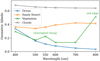 |
Fig. 3 Geometric albedos AG of model planets that are completely covered by ocean (blue), sandy desert (orange), vegetation (green), or clouds (gray). Rayleigh scattering by the gaseous atmosphere is included. |
2.3 Surface-type and Cloud Maps
The positions of the facets on the planet are determined by the Fibonacci sphere (González 2010) instead of the HEALPix scheme (Górski et al. 2005). The Fibonacci sphere has the advantage that it allows any (even) number of approximately equal-area and equilateral facets. Through testing, we determined that 1000 facets covering the whole planet strike a good balance between capturing surface and cloud patterns while ensuring the efficiency of training the network.
To create model planets with various coverage fractions of different surface types, we use the following probability distribution for fraction x (ocean), y (desert), and z (vegetation):
 (3)
(3)
Here, δ is the Dirac-delta function. The unconditional distributions for having a fraction x ocean, and for having respective fractions x and y for ocean and desert are then
 (4)
(4)
The prior probability distribution in Eq. (3) is symmetric in the three variables and, due to its singular behavior at the edges, will generate a significant number of planets with one dominant surface type. We thus trained the network to also recognize planets that are mostly covered with one of the surface types, like water worlds or desert planets.
To create a surface map on the sphere, we draw numbers q1, q2 from the uniform distribution on [0,1] and compute the fractions as follows:
 (5)
(5)
We then assigned to each facet a fictional elevation using the tetrahedral subdivision method (with an offset exponent q of 0.5) that was originally designed for video game applications (Mogensen 2010). We created surface maps by establishing the elevation cut-off levels of each surface type based on the coverage fractions x, y, and z with the ocean at the lowest elevations, vegetation at the highest, and desert at those in between.
The clouds overlay the surface and to select the facets of our model planets that are cloud covered, we draw a cloud coverage fraction from the probability distribution in Eq. (5), and then use the method described in Rossi et al. (2018) to create patchy, zonal cloud patterns. The clouds have an optical thickness of 10 at 550 nm, and the surface below them is assumed to be black. The clouds are static with respect to the surface across all epochs. A sample model planet with a surface coverage resembling Earth, thus with (x, y, z) ≈ (71%, 13%, 16%), is shown in Fig. 6.
Once we have the planet’s surface and cloud map, we compute the starlight that is reflected by each facet and, by summing the contributions of the individual facets, by the planet as a whole (see Rossi et al. 2018).
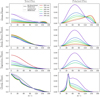 |
Fig. 4 Total flux (left column) and polarized flux (right column) phase functions of horizontally homogeneous model planets covered by ocean (first row), sandy desert (second row), vegetation (third row), or clouds (fourth row), from 400 to 800 nm. The total fluxes have been computed for Lambertian reflecting (dotted lines) and bidirectionally reflecting planets (solid lines), and the polarized fluxes only for bidirectionally reflecting planets. The curves are normalized such that a white Lambertian reflecting planet at α = 0° has a total flux of one. Near α = 180°, the approximation that the surface and atmosphere are locally plane-parallel breaks down (because of the very low fluxes, this is not visible in the curves). |
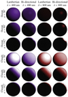 |
Fig. 5 Images of homogeneous, Lambertian and bidirectionally reflecting planets for λ = 400 and 800 nm, with the star to the top-right of each planet. A white facet corresponds to a brightness of ≥ 0.62 (normalized to a white, Lambertian reflecting facet). The overall brightest facet (2.7) is in the ocean glint for α = 142° and λ = 800 nm. At the same α and λ, the cloudy facets reach a maximum brightness of 1.1. |
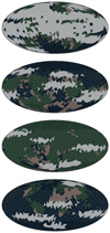 |
Fig. 6 Examples of model-planetmaps used to train the neural network, including a model Earth (bottom) with (x, y, z) ≈ (71%, 13%, 16%) in Eq. (5), and a selected cloud pattern. The flux curves of the model Earth in an edge-on orbit (i = 90°) are shown in Fig. 7. The RGB color values of each surface type are given by the albedos at the wavelengths of 700, 550, and 500 nm (see Fig. 3), respectively. |
2.4 Orbits and Rotation Axes of the Model Planets
Exoplanets move in planes that are generally observed at an angle. The inclination angle i of this orbital plane is defined as the angle between the normal on the plane and the direction toward the observer. As the planet orbits its star, α ranges from (90° − i) to (90° + i). Figure 2 illustrates planetary orbits for the values of i that we used to simulate the observations of the model planets for training and testing the network: i ranges from 0° to 90° with steps of 15°. Since we consider directly detected exo-planets, the inclination angles of their orbits could be obtained from the observations and will be provided to the network.
Rather than continuous measurements throughout a complete orbit, we assume that each model planet is observed at eight locations along its orbit, see Fig. 2. For our application, we assume that an exoplanet will be observed spatially resolved from the stellar flux, as the latter will be several orders of magnitude larger and exhibit its own temporal variations. We thus exclude small and large phase angles, where the angular distance between the planet and the star is smallest, from our simulated observations, and only include locations where 38° ≤ α ≤ 142°. For real observations, the limiting phase angle range, or the inner working angle (IWA), depends on the telescope and for example on the use of a coronagraph or a star shade, and on the characteristics of the planetary system such as the angular distance between the planet and the star. With our choice, we are on the safe side.
The lower limit of 38° ensures the visibility of the rainbow of starlight that has been scattered by liquid water cloud particles, which could be used for the characterization of clouds (for example Karalidi et al. 2011). The orbits with i < 52° do not include the rainbow location and we distribute the observation epochs evenly along those orbits, in steps of 45° around the star (see Fig. 2) to allow the observer to sample all parts of the surface. For the orbits with i ≥ 52°, we chose two observation locations at α = 38° and two at α = 142°, and the other four locations are distributed evenly along the remaining orbit. The location of each observational epoch with the corresponding value of α is listed in Table 1. Since changing the orbital eccentricity and radius alters only the magnitude and timing of the phase curves, we used circular orbits with r = 1 and F0 = 1.
An exoplanet’s rotational period and axis of rotation modulate the observed light curves and must therefore be retrieved to map an exoplanet’s surface (Kawahara 2016). We used a set of rotation axes that are homogeneously distributed across a unit sphere’s surface defined in the Cartesian coordinate system as (x, y, z) (see Fig. 2), as this prevents the neural networks from learning a bias. Because the neural networks cannot resolve the degeneracy described in Sect. 4.1, the degenerate counterpart of each rotation axis is also included in the set. To achieve this, the first 32 points from a 64-point Fibonacci spiral (see González 2010) as well as their degenerate counterparts (found by multiplying element-wise by (−1, −1,1)) create a set of 64 axes.
At each of the eight observation locations, the model planet is observed eight times as it rotates about its axis, for a total of 64 observations per orbit (we used a constant phase angle at each location, neglecting the orbital motion). During each observation, the planet is assumed to have a fixed orientation. We thus do not include rotation during the integration period (see also recommendation vi in Sect. 8). This approach reduces memory requirements for storing the phase curves, simplifies the network architecture, and increases neuron gradients, leading to more efficient training of the neural network.
Figure 7 shows the total and polarized fluxes of the Earthlike planet shown in Fig. 6 in an edge-on orbit (i = 90°) and with a rotation axis angle of 90°. Curves are shown both for a Lambertian and a bidirectionally reflecting model planet. Since the Earth-like planet is largely covered with ocean and clouds, the Lambertian and bidirectional curves differ significantly in magnitude, particularly when α = 38°, and when α = 142° (see Table 1). This was to be expected from the reflection patterns of the spatially resolved planets shown in Fig. 5.
Phase angle α vs. observational epoch and orbital inclination.
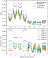 |
Fig. 7 Total (top) and polarized (bottom) flux curves for our model Earth (bottom of Fig. 6) in an edge-on orbit with an axial tilt angle of 90° (see Table 1 for the planet’s position and phase angle during each observational epoch). The polarized flux is calculated only for the bidirectionally reflecting planets, since Lambertian reflection is unpo-larized. |
2.5 Photon Noise
Because the light fluxes reflected by exoplanets will be very low, the measurable signals will have relatively strong noise levels. Most exocartography research uses Gaussian noise (for example Asensio Ramos & Pall6 2021), which can be compared to instrumental noise. In that case, however, the noise level is not adjusted to the magnitude of the flux, which can give negative values when the flux is low. Instead we used Poisson noise (also called photon noise). To calculate the noise in the total and polarized fluxes, we write the observed fluxes Io, Qo, and Uo as functions of the linearly polarized fluxes Ix, with x the angle of the optical axis of the linear polarizer through which the flux was measured (see Eq. (1.6) of Hansen & Travis 1974):
 (6)
(6)
where Ix can be derived from the numerically simulated noise-free fluxes I, Q, and U using Eq. (1.5) from Hansen & Travis (1974) (and ignoring circularly polarized flux V):
 (7)
(7)
For each noise-free flux Ix, we then computed the corresponding number of photons by multiplication with Nmax, the number of photons that would be received from a white Lambertian planet at full phase (α = 0°) without noise. Then the noisy Ix are obtained by drawing from Poisson distributions, and the observed, noisy Io, Qo, and Uo are computed using Eq. (6). The result of adding two Poisson-distributed variables with averages N = μ1 and N = μ2 is a Poisson-distributed variable with N = μ1 + μ2, so Io is also described by a Poisson distribution. When subtracting two independent Poisson-distributed variables, such as for computing Qo and Uo, one obtains a so-called Skellam distribution with mean μ1 − μ2 and variance μ1 + μ2. The distributions we used are shown in Fig. 8 for μ1 = μ2.
The effect of noise on flux curves can be seen in Fig. 9, where we show simulated total and polarized flux curves for eight rotational phases (thus at a single orbital position) assuming different photon numbers and thus different noise levels. Because polarized fluxes are generally much smaller than total fluxes (see Fig. 7), they are more sensitive to photon noise. This is particularly obvious when comparing the curves for Nmax = 103 in the two graphs of Fig. 9: while for the total flux this curve almost coincides with the Nmax = ∞ (“no noise”) curve, for the polarized flux the difference is large except at the highest flux level (Nmax = 105). Indeed, for the polarized flux to be reliably observed, we would need Nmax ≈ 2 · 104.
The number of reflected photons received by a telescope from a white Lambertian planet at α = 0° can be derived starting with Eq. (2) and using  for the reflection by the Lambertian planet (see for example Stam et al. 2006; van de Hulst 1957):
 (8)
(8)
Here,  is star’s photon emission rate across the spectral band under consideration, tinteg.. is the integration time, D is the distance between the telescope and the star system, and rtel., r, and d are the respective radii of the telescope’s primary mirror, the planet and the planetary orbit.
In the following, we assume that the planet is Earth-sized and orbits its solar-type star at a distance of 1 au. The integration time tinteg.. is 3 h (24/8 h/observations), and the spectral bandwidth is 50 nm. The stellar flux across each spectral band is computed assuming black-body radiation and a stellar radius and effective temperature of, respectively, 695 700 km and 5772 K, similar to solar values. Figure 1 shows that the number of photons Nmax reflected by a white, Lambertian reflecting planet in the Alpha Centauri system would range from 105 to 106. As we show in Sect. 6.3, Nmax should be 104 or more for accurate retrievals. According to Eq. (8), this should be achievable for systems up to distances of 20 lightyears with the Nancy Grace Roman Space telescope (in combination with a star shade) and 30 lightyears with the HabEx telescope.
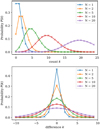 |
Fig. 8 Distribution functions for photon noise. The Poisson distributions with mean N (top) give the probability for k photons being received from a light source (such as a reflecting planet). The Skellam distributions (bottom) give the probability for the difference of two independent Poisson-distributed variables, describing the polarized fluxes Q and U. |
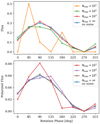 |
Fig. 9 Total (top) and polarized (bottom) flux curves at various noise levels. The number of photons that represents a total flux equal to 1.0 (a white Lambertian planet at α = 0°) is Nmax; the range of Nmax used for the polarized flux differs from that used for the total flux, because the former is generally smaller than the latter (cf. Fig. 7) and thus more sensitive to noise. The curves labeled “no noise” (Nmax = ∞) are sine functions with similar amplitudes as the curves in Fig. 7. |
3 Method: Neural Networks
3.1 Training Our Neural Networks
Our neural networks are trained by feeding them data of model planets and by comparing the networks’ output to each model planet’s true rotation axis orientation and surface map. The training data consists of numerically simulated observations of model planets with various surface and cloud maps, inclinations and rotation axis angles. These input values are multiplied by neuron weights that are adjusted by an optimization algorithm minimizing the loss, defined by the difference between the desired output and the network’s output. This process is repeated in epochs until the optimization algorithm no longer increases the network’s accuracy. The latter is established by evaluating the loss of the network when applied to validation planets, that is model planets that were not included in the training data set.
The large parameter space requires a large training data set. To reduce computation and memory requirements, we defined a set of possibilities for each of the parameters. The set size of each of the four parameters is listed in Table 2, resulting in a total of 44.8 billion unique combinations. We rapidly created 4 million model planets by randomly drawing combinations from the sets. For these planets we then computed flux curves that is the input to the network. One tenth of the planets and light curves are used for validation, to evaluate the accuracy of the neural networks.
Number of combinations for which we created model planets.
3.2 Periodic Convolutions
Recently, 1D convolutions have been used to process time-series in neural networks, achieving state-of-the-art results in fields such as biomedical data classification and early diagnosis, and anomaly detection in power electronics and electrical motor fault detection (Kiranyaz et al. 2021). Our neural network architecture uses such 1D convolutions, adjusted to take advantage of the periodic nature of the light curves. Since the model planet’s prime meridian (the line of 0° longitude) is arbitrary, the relationship between the rotational phases of, for example, 315° and 0° should be equivalent to that between 45° and 90°. To prevent that such combinations are interpreted as being distinct by the neural network, the first N − 1 rotational phases are appended to the end of each light curve before the 1 × N convolutional kernel slides over the light curve, as shown in Fig. 10 for a kernel size N of 4. An additional advantage is that the convolution does not change the dimensions of the light curve. There is thus no need for zero-padding, a common method for preserving data dimensions by adding a border of zeros around the actual data, which has the disadvantage of increasing susceptibility to spatial bias, as shown by Alsallakh et al. (2021).
To down-sample the data dimensions, a stride greater than 1 can be used. However, the kernel size should be a multiple of the stride to avoid some rotational phases being sampled more than others. We used a kernel size of 1 × 4 and a stride of 2 in the final architecture and found that the loss of the neural network decreases by 10% when using these periodic convolutions rather than conventional 1D convolutions.
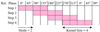 |
Fig. 10 Periodic convolution with a stride of 2 and kernel size N of 4. Since the rotational phases are pseudo-periodic, the first N − 1 values are appended to the end of the light curves before the size N kernel slides over to preserve dimensions. |
3.3 Spherical Convolutions
Originally developed for image recognition (Lecun et al. 1989), 2D convolutions can also be used for 2D image generation, for example when generating faces (Karras et al. 2020) or for semantic segmentation, where the output of the neural network is an image with each pixel belonging to a specific class (Wang et al. 2018). Asensio Ramos & Pall6 (2021) demonstrated that convolutions on the surface of a sphere can be used to regularize retrieved exoplanet maps. They use the spherical convolution algorithm developed by Krachmalnicoff & Tomasi (2019) combined with ReLU activation functions to regularize a retrieved planet map on a HEALPix pixelization scheme (Górski et al. 2005).
Since we did not use HEALPix but a Fibonacci sphere, we have adapted the spherical convolution algorithm by Krachmalnicoff & Tomasi (2019). A spherical convolution takes advantage of the optimization that has been achieved for 1D convolutions by expanding the 1D list of facets on the sphere’s surface such that each facet is followed by its N surrounding facets. Then a kernel with size and stride equal to N + 1 convolves each facet with its surrounding facets. To achieve this for a Fibonacci sphere, we first identified each facet’s surrounding facets. These are then ordered in clockwise direction by calculating the clockwise angle from the z-direction to each surrounding facet’s center. More rings can be added by taking the surrounding facets of the inner ring. A problem that arises here is that the rings around the facets have different sizes, while the 1D kernel can only have one size. To solve this problem, Krachmalnicoff & Tomasi (2019) use zero-padding, which can cause unwanted artifacts (Alsallakh et al. 2021). To avoid these artifacts, we instead used the periodicity of the rings and add the first value to the end of the series. Then we computed the mean integer length of the rings surrounding each facet, and if the number of facets in a given ring differs from the mean value, facets are either repeated or taken out in an evenly spaced manner. This can yield gaps in the rings as shown in Fig. 11, while in other places there can be double counts, causing spatial bias with minimal effects on the final maps.
4 Results: Retrieval of the Rotation Axis
The first step for retrieving planet maps using reflected fluxes is to estimate the orientation of the planet’s rotation axis. Fujii & Kawahara (2012) find the axis orientation by maximizing the overlap between the measured signals and dominant left-singular vectors. Kawahara (2016) also showed that retrieval of the axis is possible from measurements of the frequency modulation of the planetary signal over a complete orbit. Because we take eight discrete observational periods of a planet along its orbit instead of (near) continuous monitoring, we decided to use a convolutional neural network approach with as output of the network the three Cartesian coordinates of the planet’s rotation axis.
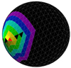 |
Fig. 11 Example of a spherical convolution with five rings. The method developed by Krachmalnicoff & Tomasi (2019) (originally for HEALPix) is adapted to the Fibonacci sphere with the improvement that instead of zero-padding, the periodic nature of rings is used. Some facets inside the rings are black because they are not included in the kernel, since the number of facets in each respective ring must match for all kernel locations on the sphere. |
4.1 Degeneracy in the Signal for the Edge-on Case
The retrieval of the rotation axis is problematic when the orbital inclination angle i is close to 90°, because then every configuration has a mirror configuration with the same light curve upon reflection in the orbital plane, as the orbit and the sense of rotation remain the same. However, this leaves the planet map mirrored with respect to the equator and the x and y components of the rotation axis change sign. In the reference system shown in Fig. 2, this would be expressed as an element-wise multiplication by (−1, −1,1). Because the two configurations are inherently different, while the observable light curves are identical, the neural network should not be able to decide on the actual configuration. We identified the degeneracy by trial-and-error and confirmed by testing that the light curves are the same for several different mirror pairs.
4.2 Architecture
We drew inspiration for our neural network architecture, shown in Fig. 12, from other convolutional signal processing neural networks (see, for example, Badshah et al. 2017). We split the network into a “feature recognition” part with convolutional layers followed by a “feature combination” part with dense linear layers. The network must be retrained for each new orbital inclination angle i.
The input dimensions to the neural network are either 8 ☓ 8 ☓ 6 without polarization (8 orbital locations, 8 rotational phases, 6 wavelengths) or 8 ☓ 8 ☓ 12 with polarization (Stokes parameters I and Q are included, which doubles the final dimension; parameters U and V have negligible magnitudes and are not included in the retrievals). The network’s feature recognition part consists of two periodic convolutional layers, each with 16 filters. The first layer, with a kernel size of 3, increases the dimensions of the input to 8 ☓ 8 ☓ 16, as shown in Fig. 12. The final dimension increases to 16 since each of the filters, which convolve the six wavelengths and eight rotational phases, has its own output. To halve the size of the data, the second periodic convolution skips half of the rotational phase steps (stride = 2) with a kernel size of 4, leading to an 8 ☓ 4 ☓ 16 output, as shown in Fig. 10. The output of the last convolutional layer is then flattened and passed onto the network’s feature combination part.
The data is then fed through five dense, fully connected layers with linear activation functions and a bias. These layers have 512, 512, 256, 32, and three nodes, respectively. The first four layers are followed by PReLU activation functions to introduce nonlinearity (He et al. 2015):
 (9)
(9)
where the slope coefficient ai causes nonlinearity due to the change in gradient at yi = 0 and is actively learned and manually inspected (see Fig. 13). To prevent over-fitting, the first three layers are followed by dropout regularization layers with a dropout rate of 15%. These dropout layers randomly set 15% of the layer’s output to 0, preventing the neural network from over-fitting to peculiarities of the training data. The network has a total of 667, 907 or 667, 619 trainable parameters, depending on whether polarization is included or not, respectively. The parameters that we trained are the weights of the convolutional kernels, linear nodes and slope coefficients of the PReLU layers.
4.3 Training the Axis Retrieval Network
When the neural network is trained on all planets with a given inclination angle i, the available number of light curves is 4000000/7 ≈ 570000. In order to mitigate the degeneracy (Sect. 4.1), the network can only be trained on all planets with a rotation axis with y ≥ 0, in which case the number of curves is halved. We used 90% of the curves for training and 10% for validation. To prevent over-fitting, we stopped with training when the validation losses have not decreased for two consecutive epochs.
The neural network is created and trained using the Keras Python package.4 Since retrieving the rotation axis is a regression problem, we chose the mean squared error (MSE) as the loss that the network should minimize. We found that for small batch sizes (16 to 64 planets fed to the neural network together), the training loss can increase after roughly ten epochs. This appears to indicate that the optimization algorithm (Kingma & Ba 2014) overshoots the local minimum and adjusts to peculiarities in the small batch, rather than finding the global optimum. This problem was solved by increasing the batch size to 256.
Figure 13 shows the slope coefficients a (see Eq. (9)) after training for the edge-on case. The coefficients of PReLU layers 2, 3, and 4 are distributed around zero. Because they approximate a classical ReLU function with a = 0, we tested replacing them with ReLU layers, but this did not lead to better results as the validation losses of this modified network were larger; apparently the nonzero a values in these PReLU layers do add value. PReLU layer 1 is not centered around zero but has a mean a of −0.32, with a standard deviation that is roughly one order of magnitude larger than that for the other layers. The negative coefficients of the majority of the nodes in layer 1 mean that the PReLU function is not one-to-one.
4.4 Numerical artifacts
When the network is trained with light curves with very little noise, it can distinguish between the two degenerate cases addressed in Sect. 4.1 and correctly estimate the x and y coordinates of the planet’s rotation axis. Because this information should actually not be present in the light curves, this shows that the network uses numerical artifacts in the retrieval. For example, the network might have learned to recognize the facet scheme, which is not symmetric under the reflection in the plane.
By increasing the noise levels, such numerical artifacts are suppressed. We have determined by trial and error that a noise level at photon numbers Nmax ≈ 104 ensures that the network is unable to distinguish the degenerate cases, as it should be.
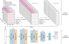 |
Fig. 12 Network architecture to retrieve rotation axes. The feature recognition part uses periodic convolutions and the feature combinations part consists of densely connected layers with PReLU activation functions and dropout layers to prevent over-fitting (the number of nodes is indicated above the lower layers). When using polarization, the input shape is 8 ☓ 8 ☓ 12, otherwise 8 ☓ 8 ☓ 6. The periodic convolutions maintain the 1st and 2nd data dimensions since the first N − 1 values along the rotation axis are appended to the end before convolution. The number of filters determines the 3rd dimension of the output. The number of trainable parameters is 667907 (with polarization) and 667619 (without polarization). |
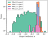 |
Fig. 13 PReLU slope coefficients after training (plotted with a log scale). See Fig. 12 for the position of each layer in the neural network. These coefficients were retrieved from a neural network trained on planets in an edge-on orbit with bidirectional light curves and including polarization. |
4.5 Retrieval Accuracy for Near Edge-on Observations
The left panel in Fig. 14 shows the retrieval accuracy of the neural network as a function of the orbital inclination angle i. The loss increases with i up to MSE = 0.22 for i = 90°, except for the network that was trained with Lambertian data but that was presented directional validation. Here, the degeneracy in the geometry happens: the network cannot determine the signs of the x and ycomponents of the rotation axes. In that case the retrieved values are near zero and therefore
 (10)
(10)
The degeneracy for the near edge-on observation can be mitigated by constraining the rotation axes to y ≥ 0 and by training the neural network on these planets only. The neural network is able to approximate the rotation axis in this half of the search space, as shown in Fig. 15. With decreasing inclination angle, the two cases y > 0 and y < 0 are increasingly distinguishable, and the use of a constraint becomes invalid, as by then giving away the correct sign of y, one obviously artificially reduces the MSE.
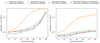 |
Fig. 14 Rotation axis retrieval accuracy as a function of orbital inclination angle i without (left) and with the constraint y ≥ 0 (right). Blue: training with Lambertian reflection and retrieval with Lambertian reflection; Orange: training with bidirectional reflection and retrieval with Lambertian reflection; Green: training with bidirectional reflection and retrieval with bidirectional reflection, both without polarization; Red: the same, but both with polarization. |
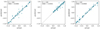 |
Fig. 15 Accuracy of the retrieval of the rotation axis direction for N = 100 model planets in edge-on orbits: the x-coordinate (left), y-coordinate (middle), and z-coordinate (right). The degeneracy has been mitigated with the constraint y ≥ 0. |
4.6 Retrieval Accuracy at other Inclination Angles
The network is trained three times, for three different reflection models. First, we trained it with light curves computed assuming Lambertian reflection. The second and third training sessions are with light curves computed using bidirectional reflection with and without polarization. All losses discussed in this section are validation losses, and thus the network’s losses when it is applied to the validation planets that it was not trained with.
4.7 Validation with Model Earth
In order to validate that the neural network is able to retrieve maps and rotation axes of planets that are not included in the training data, we used calculated data of the cloudy model planet Earth shown in Fig. 6. The fluxes were computed using bidirectional reflection with polarization for a face-on orbit (i = 0°) with rotation axis coordinates (0.918,0.281, −0.281), such that the tilt is 23.4°. Noise corresponding to Nmax = 104 photons was added to the fluxes and they were normalized to a maximum value of 1. The network trained on planets with rotation axes with y ≥ 0 predicts a rotation axis of (0.904,0.170, −0.331) for the light curves, corresponding to an MSE of 0.0050, similar to the MSE obtained from the validation for face-on orbits. We conclude that the neural network has not “memorized” the maps or rotation axes in the training data and constrains the rotation axis as intended.
5 Results: Retrieval of Albedo Maps
5.1 Absolute Light Curves
In this section, we attempt to replicate the results of other authors, retrieving planetary albedo maps based on absolute light curves computed using Lambertian reflection (see for example Fujii & Kawahara 2012; Kawahara & Masuda 2020; Fan et al. 2019; Farr et al. 2018; Asensio Ramos & Palle 2021). Since information about facets that never face the observer is not present in the light curves, the neural network cannot retrieve the albedos of those facets. The number of output albedo values is thus between 500 (the axis is parallel to the line of sight and only half of the surface becomes visible) and 1000 (the axis is perpendicular to the line of the sight and the whole surface becomes visible). Every facet that becomes visible also becomes illuminated while being visible.
Since the problem is linear in nature, the first architecture that is tried is a single layer of nodes (see Table 3), meaning that each facet output is a linear combination of the 64 flux values (8 orbit locations ☓ 8 rotation phases). Since no facet is biased toward a high or lower albedo, it is found that including biases in the nodes decreases the retrieval accuracy.
The neural network is trained using Lambertian, absolute flux curves for an orbital inclination of 60° and a rotation axis of (0.93, −0.20, −0.30) (this geometry is found to be best in Sect. 5.2). The wavelength chosen for the retrievals is 550 nm, since at this wavelength it is easiest to distinguish the four surface types from each other (see Fig. 3). Furthermore, 10% of the data is used as validation data, the batch size of the training is set to 32 (found by trial and error to be optimal), the network is trained until the loss does not decrease for 10 consecutive epochs and the loss function used is the mean squared error (MSE) since this is a regression problem. These training parameters are used for all architectures discussed in this section.
The validation loss of the single layer after 413 training epochs is 0.0186. By trial and error, it is found that adding another layer of 64 nodes decreases the MSE to 0.0164 while also roughly halving the number of training epochs to 249. Adding more dense layers than this does not further decrease the validation loss of the network. However, the accuracy can be improved by including a periodic convolution (described in Sect. 3.2) with a kernel size of 1 ☓ 3 before the two densely connected layers. The MSE of this model when applied to the validation data is equal to 0.0146. Two example retrievals are shown in Fig. 16 for a model planet Earth in the best and worst configurations of inclination and rotation axis shown in Fig. 17.
Tested architectures for retrieving facet albedos.
5.2 Retrieval Accuracies for Different Geometries
In this section, the effect of the orbital inclination angle and the rotation axis orientation on the albedo map retrievals is investigated. Only half of the possible 64 rotation axes are discussed since all axes with x ≤ 0 can be reflected in the yz plane to create a new axis with the same observations in reverse order, resulting in the same retrieval accuracy (see Fig. 2 for the definition of the ( x, y, z) coordinate system).
To this end, the final model from Table 3 is retrained for all 32 axes with x ≥ 0 for each of the seven inclinations (0°, 15°, 30°, 45°, 60°, 75° and 90°). The resulting MSEs of the validation data are plotted in Fig. 17. The number of facets that are retrieved varies for each rotation axis, since not all facets become visible.
We found that a rotation axis angle (angle between the rotation axis and orbital normal vector) near 90° provides the best retrieval accuracy for edge-on and near-edge-on orbits (i = 75° and i = 90°). For edge-on orbits (in the xy plane), the orbital movement modulates the signal across the y (vertical) axis of the planet’s surface. When the rotation axis has a large component in the orbital plane, this provides modulation in the opposite (z) direction. Conversely, when the axis is normal to the orbital plane the modulation due to the rotation of the planet is in the same direction as the modulation due to the orbital movement. Edge-on orbits with rotation axes normal to orbital plane thus have the worst accuracy of all combinations. The worst geometry that is studied is for an edge-on orbit and a rotation axis of (0.34, −0.11, −0.94), with an MSE of 0.022.
For face-on and near-face-on orbits, the orbital movement of the planet modulates the signal in both the y and z directions. The best retrieval accuracies are then found for axes near the normal of the orbital plane that also modulate in both directions. Axial tilts near to 90° modulate in only one direction and thus show slightly worse results. The best geometry is found for an inclination of 60° and an axis of (0.93, −0.20, −0.30), as in this case the orbit and rotation axis both modulate across two perpendicular directions. The rotation axis angle is 78°, so the rotation axis lies close to the orbital plane, roughly in the direction of the observer. The MSE for this case is 0.015 and this geometry is chosen for many of the remaining example retrievals in this paper.
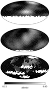 |
Fig. 16 Examples of albedo map retrievals for the best (top) and worst (middle) geometries from Fig. 17 using absolute light curves for λ = 550 nm. In these cases, 681 and 917 facets are visible, respectively. The map outside the visible region is white. The original map (bottom) is the model Earth (at λ = 550 nm). The MSE for these two retrievals is 0.0286 and 0.0129, respectively, which is similar to the MSE of the validation data for these geometries (see Fig. 17). |
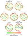 |
Fig. 17 Accuracy of albedo retrievals using the last architecture from Table 3 for various combinations of rotation axis and inclination. The axes are shown from the observer’s perspective. Only the 32 axes with x > 0 (on the front-side) are shown since the other 32 axes are mirrors with the rotation epochs in reverse order. The highest loss is found for i = 90° and an axis of (0.34, –0.11, –0.94), and the smallest loss for i = 60° and the axis of (0.93, –0.20, –0.30). |
5.3 Relative (Normalized) Light Curves
Since the radius of an exoplanet is difficult to constrain from direct detections (a small, bright planet can have the same flux as a large, dark one), we used flux curves that are normalized to 1.0 for our retrieval algorithms for directly observed exoplan-ets. To this end, we used a modified architecture as shown in Fig. 18 in which the outputs of the periodic convolution are used to estimate the overall brightness of the albedo maps by three densely connected layers with 32 nodes each. Two single nodes (which each output a single value) are then multiplied and added to the albedo map to scale the map to the estimated brightness. The densely connected layers have ReLU activation functions, which are a special case of PReLU (Eq. (9) with a = 0). Based on our experience with this architecture, PReLU layers where a is actively trained instead of ReLU layers do not provide better results and increase the number of epochs needed to reach a similar validation loss.
When using the network designed for absolute flux curves (Table 3) and training it with normalized flux curves, the MSE increases from 0.0146 to 0.0197. Using the scaling discussed above decreases the MSE from 0.0197 to 0.0162. This shows that the network can effectively estimate the map’s brightness.
Mean squared error (MSE) of the albedo retrievals.
5.4 Effects of Noise
In this section, we study the effect of noise on the albedo map retrievals. We trained the architecture from Fig. 18 with normalized, Lambertian light curves with different levels of photon noise added (see Sect. 2.5). The MSE of the validation data and the retrieved model Earth maps are shown in Table 4 and in Fig. 19. For all noise levels the retrieval of the model Earth is significantly better than that of the validation data. This could be because the model Earth is largely covered by vegetation and ocean, which have similar albedo’s for the studied wavelength of 550 nm when compared with a combination of clouds and ocean, for example. Homogeneous planets may be easier to retrieve since there are less hard-to-predict details with large penalties for the loss function.
For the case without noise (Nmax = ∞), the clouds, the Sahara and North America can be clearly distinguished. These features disappear at a noise level corresponding to Nmax ≤ 103 photons. The results shown here are comparable to results from Fujii & Kawahara (2012); Farr et al. (2018); Fan et al. (2019); Kawahara & Masuda (2020); Asensio Ramos & Pallé (2021), although a precise comparison is difficult due to differences in geometry, noise models, number of observations and the specific map.
6 Results: Retrieval of Surface-Type Maps
Since albedo maps do not fully describe the properties of a planet and do not identify unique non-Lambertian reflecting patterns due to oceans and clouds, we here retrieve for each facet that covers the planet, a surface type instead of an albedo, as in Sect. 5. The four possible surface types for each facet are: ocean, vegetation, sandy desert, and clouds (while strictly speaking clouds are not on the surface, the network assumes them to be). For each facet, our neural network predicts a probability for each surface type. When creating maps or checking the classification accuracy, each facet is assigned the surface type with the highest probability.
6.1 Architecture
To create surface type maps, the output dimensions of the neural network should equal the number of visible facets (between 500 and 1000) times the number of possible surface types (4). To recognize patterns in the light curves, we used a similar periodic convolution as shown in Fig. 12. Two periodic convolutions (see Sect. 3.2) with 16 kernels of size 1 × 3 and 1 × 4 were applied to the light curves. No down-sampling was done as the resolution along the rotation phase should be high to create accurate maps; the stride is thus 1. This means that we used a vector of size 1024 after flattening the output of the periodic convolutions. This was followed by a dense layer for each surface type. Each dense layer has as many nodes as there are output facets.
Finally, we used spherical convolutions to regularize the surface map. With a ResNet approach (He et al. 2016) the dense layer output is fed into the convolutions (four filters, one ring) and the output is added to the previous output. This is repeated five times to achieve the final output of the neural network. Before training, the spherical convolution kernels were initialized with zeros, to avoid interference with the learning of earlier layers.
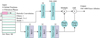 |
Fig. 18 Architecture used to retrieve planetary albedo maps from normalized phase curves. Several logic layers with ReLU activation functions are used to scale the output map by adding and multiplying by two single values. The scaling part of the network decreases the loss from 0.0197 to 0.0162 (for the ideal geometry as shown in Fig. 17). The output of the neural network is between 500 and 1000 values, depending on the number of facets that is visible for the specific geometry. Neurons in the bottom layers have biases but neurons in the top layers do not. |
6.2 Training the Surface-Type Network
The neural network was trained for one combination of inclination and rotation axis at a time, so the training data consists of roughly 4000000/7/64 ≈ 9 000 light curves, of which 10% were set aside for validation. The neural network was trained using the Adam optimization algorithm (Kingma & Ba 2014), until the validation loss did not decrease for five consecutive epochs. We found that a batch size (number of training curves fed into the neural network simultaneously) of 32 works best, since larger batch sizes can cause the network to overshoot the local minima. This could be due to the gradient magnitudes in combination with the standard learning rate in Keras. We also found that training the neural network using the MSE as the loss function gives the highest retrieval accuracies when compared to the categorical cross entropy that is usually used for classification problems (Zhang & Sabuncu 2018). This might be due to the ill-defined nature of the exocartography inversion problem or to a suboptimal network architecture.
6.3 Retrieval Accuracy
In this section, the retrieval accuracies of the neural network architecture shown in Fig. 20 are investigated. The retrieval accuracy of each surface type is plotted as a function of the noise level in Fig. 21. The inclination and rotation axis chosen were the best combination as shown in Fig. 17. Since the inclination angle is 60°, the rainbow feature at α = 38° is visible at two of the eight orbital positions and the ocean glint is also prominent at the two orbital positions for which α = 142°.
The network performs poorly when trained on Lambertian light curves while applied to directional light curves. This will be further discussed in Sect. 7.2. The surface type that is correctly classified most often is ocean, due to its unique glint feature as well as its characteristic darkness. We verified that the high accuracy is (at least) partially due to the ocean glint since the Lambertian trained network applied to Lambertian light curves does not perform as well as the directional trained network applied to directional light curves. A similar effect is also seen for cloudy facets, which also have unique, bidirectional reflection (see Fig. 4). The accuracy of the classification of vegetation and desert surface types, which are modeled as Lam-bertian reflectors, does not increase when bidirectional curves instead of Lambertian curves are used. We found that excluding the light curves with a wavelength of 550 nm (the green bump) does not impact the retrieval accuracy of the surface maps in the absence of noise.
The retrieved maps of the Earth-like planet are shown in Fig. 22 for different noise levels. These maps have more detail than the albedo maps shown in Fig. 19, which validates our approach of retrieving surface types rather than albedos. In the absence of noise (Nmax = ∞), all continents can clearly be distinguished. At a noise level for photon numbers Nmax ≤ 103, the Americas disappear. Lastly, for Nmax = 10, only the main surface types (vegetation and ocean) are retrieved. At this high noise level, the retrieved map depends strongly on probabilistic noise contributions.
7 Discussion
Our method of retrieving exoplanet surface maps is based on the assumption that the planet has an atmosphere with clouds and three surface types: ocean, desert and Earth-like vegetation. These are modeled with bidirectional reflection for clouds and a rough ocean with glint. The planet has a fast rotation compared to the orbital period, as its surface is static. Here, we first discuss the results of using neural networks, then the results from our inclusion of bidirectional reflection and polarization in the signal, and list possible steps for an observational campaign and recommendations for future work.
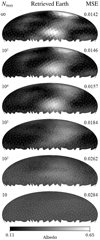 |
Fig. 19 Albedo retrievals of an Earth-like planet for different noise levels (Nmax = ∞ is noise-free), using the optimal configuration from Fig. 17. The architecture from Fig. 18 for total flux curves computed using Lambertian reflecting model planets is used. The actual Earth albedo map is shown in Fig. 16. The MSE is computed by comparing the retrieved map with the map of the model Earth. |
7.1 Optimizing the Neural Network Architectures
The rotation axis retrieval is nonlinear and therefore a neural network with nonlinear activation functions was found to be most accurate. On the other hand, the neural network for creating surface-type maps was found to work best when only linear layers were used, contrary to our initial assumptions. The linear neural network is equivalent to a least squares method (with regularization) which defines the ideal solution for a data set. It remains to be seen whether neural networks have advantages over least-squares solutions for the map retrieval with a constrained rotation axis.
Our model assumes a static map, and we thus did not include seasonal variations, such as dynamical ice caps, hurricane clouds, and volcanic eruptions. Although nonstatic maps can be retrieved with a least-squares method, this is at the cost of spatial resolution (Kawahara & Masuda 2020). Neural networks could be trained to make connections between planet characteristics, such as a relation between an obliquity of the planet’s rotation axis and the varying size of a polar ice cap, or between cloud cover and oceans. They thus appear to be suitable for the retrieval of dynamic maps, and we expect them to prove their usefulness in future exocartography.
7.2 Consequences of the Lambertian Assumption
Since all other authors, to our knowledge, use Lambertian reflection for their retrievals, it is interesting to evaluate the validity of this Lambertian assumption for training a network when the actual data will be of planets that reflect non-Lambertian, that is bidirectionally. When retrieving the rotation axis, the network trained with Lambertian curves and applied to Lambertian model planets performs best of all combinations in Fig. 14: the MSE is 0.0074 for face-on orbits. However, when this network that was trained with Lambertian model planets is applied to the more realistic bidirectional light curves, the losses increase by roughly one order of magnitude for large inclination angles. Thus evaluating the network’s performance while using only Lambertian light curves leads to a false confidence in the retrieval algorithm’s accuracy. When such a retrieval algorithm is used to retrieve the rotation axes of bidirectionally reflecting planets in a face-on orbit, however, the MSE is 0.0117, only 18% larger than the MSE of 0.0099 for the network that was trained on bidirectional curves. This confirms that in an edge-on orbit, where the phase angle is constant along the orbit, the reflection appears to be mostly Lambertian because of the lack of angular features.
The MSE of the retrievals by the networks trained with bidirectional models increases with increasing inclination angle. Including polarization in the retrievals overall increases the retrieval accuracy. The beneficial effects of including polarization are smallest for i = 0° and 15°. This can be explained since the reflected flux for these small inclinations appears to be mostly Lambertian. The largest decrease in MSE when including polarization occurs for i = 60°, where including polarization decreases the loss by 26%.
To test the Lambertian assumption for albedo map retrievals, we used the architecture from Fig. 18, which provides comparable results to those by other authors by training on Lambertian light curves and testing on directional light curves (light curves computed using directional reflection). As can be seen in Fig. 23, strong concentric artifacts about the pole appear for all inclinations besides for a face-on orbit. Each of the planets in the figure is a homogeneous planet and should be retrieved as such. Since the planets have the same flux at all rotation phases, the artifacts are purely due to the overestimation of the flux at low phase angles and underestimation of the flux at high phase angles when using the Lambertian assumption (see Fig. 4). Since most exo-planets are not in a face-on orbit, these errors demonstrate a need for new retrieval algorithms that use directional light curves to map planet surfaces.
For surface-type map retrievals, the Lambertian trained neural network yields large errors when applied to bidirectional light curves, as can be seen in Fig. 21. As an example, Fig. 24 shows the map as retrieved from bidirectional light curves of the model Earth (see Fig. 6) by a neural network that was trained on Lambertian light curves. Amongst others, the network predicts a large fraction of desert facets where there should be dark ocean facets.
Since so far we have only studied the ideal geometry from Fig. 17, we also used other inclinations to investigate if that improves the retrieval of the Lambertian trained network, like with the rotation axis and albedo map retrievals for a face-on orbit. Figure 25 shows the retrieval accuracy for Lambertian and bidirectional trained networks as functions of the inclination angle, using a rotation axis tilt close to 0°. As seen in Fig. 25, the Lambertian trained network is only reliable for orbits that are face-on or close to face-on: only for i ≤ 10° all surface types have a classification accuracy larger than 60%, and even then, the accuracy of the directional network is considerably higher and thus preferred.
The only surface type for which the classification accuracy of the Lambertian trained network is higher than 65% for all inclination angles is vegetation. Indeed, the Lambertian network can use the red edge feature in the albedo (see Fig. 3) to recognize vegetation. Since the atmospheric influence on the signal is very small at the large wavelengths of the red edge, and because vegetation is modeled as a Lambertian reflector, vegetation facets appear very similar in directional and Lambertian light curves (see Fig 4).
 |
Fig. 20 Architecture for classifying facets on a planet as one of four surface types. Several periodic convolutions recognize patterns in the curves similar to the rotation axis retrieval network (Fig. 12). To maintain a high level of resolution of rotation phases, no down-sampling is used in the convolutions. Four dense layers with 500 to 1000 nodes estimate the probability of each surface type for all visible facets. We applied five spherical convolutions in series and add the outputs to achieve the final result. We used four filters in the spherical convolutions to match the dimensions. |
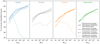 |
Fig. 21 Percentages of correctly retrieved facets in the validation data for different noise levels and different combinations of training data (Lambertian or bidirectional reflection) and validation data (Lambertian or birdirectional reflection). Ocean, clouds, desert and vegetation facets show maximal percentages of 92%, 85%, 85%, and 85%, respectively. The architecture in Fig. 20 was trained for the best combination of orbital inclination and rotation axis shown in Fig. 17. |
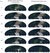 |
Fig. 22 Retrieved maps of the model Earth (bottom of Fig. 6) for different levels of photon noise, using directional light curves with (left) and without polarization (right). The architecture from Fig. 20 was used and trained for the optimal configuration of Fig. 17. For Nmax = ∞ photons, there is no noise. |
7.3 Benefits of Polarization
The effects of including polarization on the surface-type map retrievals can be seen in Table 5 which shows the confusion matrices for the bidirectional neural networks with and without polarization. Confusion matrices visualize the performance of classification schemes by showing for each actual class the fractions of the possible classes that are retrieved, thus, the fraction of ocean facets that is retrieved as ocean, desert, vegetation, and cloud facets, for example.
A comparison of the confusion matrices shows that the retrieval accuracy of the desert and vegetation-covered surface facets is insensitive to including the polarization signal to the model observations and the retrieval algorithm. This is to be expected since both surface types are modeled as Lambertian, nonpolarizing surfaces. Indeed, the retrieval accuracy of ocean and cloud facets is increased by 2% and 1%, respectively, due to the unique polarization signatures of the ocean glint and the rainbow. Including polarimetry on a future exoplanet characterization telescope would thus increase the ability to map oceans and clouds on exoplanets.
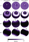 |
Fig. 23 Albedo maps of bidirectionally reflecting planets at λ = 400 nm for homogeneous desert, cloud, and ocean planets retrieved by the network architecture of Fig. 18 that was trained on Lambertian reflecting planets, for different orbital inclination angles i. The rotation axis for each planet (indicated with a white or black cross) was chosen from the set shown in Fig. 17 to minimize the difference to the normal of the orbital plane. The tilt angles of the axes are 15°, 5°, 11° and 23° in order of ascending inclination. |
 |
Fig. 24 Map of the model Earth as retrieved from bidirectional light curves by the network that was trained with Lambertian reflecting curves. The orbital inclination and rotation axis of the planet are the optimal configuration shown in Fig. 17. The actual map is shown in Fig. 6. |
7.4 Steps in Observation Campaign
We imagine that the actual observation campaign consist of the following steps. (i) Determine the orbital elements of the Kepler orbit and the period from the (relative) positions of the planet at the observation points. Feng et al. (2019) describe a comprehensive method to obtain these positions. (ii) Determine the diurnal period from light curves at (one or more) observation points and the phase shift between the points (see for example Visser & van de Bult 2015). Close-in planets can be tidally locked or in a spin-orbit resonance. These need to be treated as special cases that we do not consider in this paper. (iii) Update the parameters, and corrected for the diurnal phase shift due to the light-travel (Rømer) delay, at the different observation points. (iv) Retrieve the rotation axis as explained in Sect. 4. (v) Retrieve the surface map. This is demonstrated in Sect. 6.
 |
Fig. 25 Accuracy of the retrieval algorithms that trained on Lambertian (dashed) and bidirectionally (solid) reflecting planets, when applied to light curves of bidirectionally reflecting planets, as functions of the orbital inclination angle i. The rotation axes for each inclination angle are chosen to minimize the difference to the normal on the orbital plane (see Fig. 23 for examples). |
7.5 Recommendations
We have a number of recommendations for further research on the application of neural networks to exoplanet cartography: (i) Include more surface types in the training data, like ices (such as those found on Earth, Mars, and icy moons), differently colored deserts (such as the martian red desert), and wetlands. (ii) Implement dynamical surface maps to capture seasonal changes, for example in the size of polar ice caps, snow cover, and vegetation color, and train a network to recognize such surface types from their seasonal changes. (iii) Include different model atmospheres and different cloud compositions, such as sulfuric acid clouds as seen on Venus, that exhibit angular features, such as the rainbow, at different phase angles than water clouds (see Hansen & Travis 1974, for examples in single scattering phase functions). (iv) Include other noise sources than photon noise, such as instrumental noise and physical background noise sources. (v) Simulate with orbital and rotational periods that are closer together in frequency or in a resonance (like Mercury’s 3 : 2 spin-orbit resonance). (vi) Account for signal smearing caused by the planet’s rotation during one observational integration period. (vii) Optimize the number of sample points. Increasing the number of observational epochs may require new network architectures as the number of trainable parameters may become too large for efficient training. (viii) Test different weighting schemes for the loss function of the neural network, in particular for surface type retrieval. This would allow training to focus on facets with smaller or larger expected contributions to the phase curves. (ix) Test the retrieval algorithms with light curves of Earth observed from afar, for example by using an instrument like LOUPE (Klindžić et al. 2021) on the Moon or on a distant spacecraft. (x) Investigate how to adapt the network to identify a surface type with an unknown albedo spectrum, such as that of vegetation that uses photosynthesislike processes at other wavelengths than the terrestrial vegetation and/or that has a red edge feature at different wavelengths. One of the key advantages of neural networks is that they are flexible and show promise for implementing many of the mentioned recommendations using the same architectures presented in this paper, or improvements thereof.
8 Conclusions
We used neural networks to retrieve surface and cloud maps of spatially unresolved Earth-like exoplanets, using temporal and spectral variations in the flux and polarization of the star light that is reflected by such planets.
We were able to retrieve the rotation axes of our model planets using a neural network with 1D convolutions. The mean squared error (MSE) is as small as 0.0097 and depends on the orbital inclination angle. In the special case of an exact edge-on orbit, the signals are insensitive to mirror reflection of the axis in the orbital plane. Up to this reflection symmetry, the rotation axis can be determined.
We have tested a new approach for planet mapping by predicting surface types rather than surface albedos. A neural network with 1D convolutions and spherical convolutions applied in a ResNet fashion can create detailed planet maps that correctly predict up to 92% of ocean facets and 85% of cloud, vegetation and desert facets on a planet. When applied to a model Earth, the retrieved map shows that the Sahara, Europe, Asia, the Americas and cloud patterns can all be retrieved. When photon noise is the dominant noise source, our results show that it should be possible to retrieve a map with such Earth-like patterns from future observations by the HabEx telescope in combination with a star shade for planets at distances of up to 75 ly.
We showed that the retrieval of the rotation axis and surface map is usually poor if the network assumes Lambertian reflection for a bidirectionally reflecting planet, except for planets in face-on orbits, where the lack of phase angle variation hides the bidirectionality of the actual reflection. In particular, retrieving maps of planets with oceanic reflection and atmospheric scattering while assuming Lambertian reflection results in erroneous concentric bright patterns about the planet’s poles due to an over-estimation and an underestimation of the planet’s brightness at small and large phase angles, respectively. The MSE of the rotation axis retrievals is reduced by a factor 10 if the network does take bidirectional reflection into account.
We also showed that while photon noise affects a planet’s polarized signal more than its total flux signal, adding polarization to the neural network training decreases the MSE of the rotation axis retrievals by about 15% and increases the retrieval accuracy of ocean and and cloud-covered facets by 2% and 1%, respectively, due to their unique polarization signatures.
In conclusion, neural networks appear to be promising tools for retrieving exoplanet maps from total flux and polarization phase curves. Eight orbital locations and eight rotational phases appear to suffice for Earth-like planets when using the architectures we have discussed.
References
- Alsallakh, B., Kokhlikyan, N., Miglani, V., Yuan, J., & Reblitz-Richardson, O. 2021, in Mind the Pad - CNNs Can Develop Blind Spots, International Conference on Learning Representations [Google Scholar]
- Asensio Ramos, A., & Pallé, E. 2021, A&A, 646, A4 [NASA ADS] [CrossRef] [EDP Sciences] [Google Scholar]
- Badshah, A., Ahmad, J., Rahim, N., & Baik, S. 2017, in Speech Emotion Recognition from Spectrograms with Deep Convolutional Neural Network, 1 [Google Scholar]
- Bryson, S., Coughlin, J., Batalha, N. M., et al. 2020, ApJ, 159, 279 [CrossRef] [Google Scholar]
- Cash, W. 2006, Nature, 442, 51 [NASA ADS] [CrossRef] [Google Scholar]
- Dressing, C. D., & Charbonneau, D. 2015, ApJ, 807, 45 [Google Scholar]
- Fan, S., Li, C., Li, J.-Z., et al. 2019, ApJ, 882, L1 [NASA ADS] [CrossRef] [Google Scholar]
- Farr, B., Farr, W. M., Cowan, N. B., Haggard, H. M., & Robinson, T. 2018, AJ, 156, 146 [NASA ADS] [CrossRef] [Google Scholar]
- Feng, F., Lisogorskyi, M., Jones, H. R. A., et al. 2019, ApJS, 244, 39 [NASA ADS] [CrossRef] [Google Scholar]
- Ford, E. B., Seager, S., & Turner, E. L. 2001, Nature, 412, 885 [NASA ADS] [CrossRef] [Google Scholar]
- Fujii, Y., & Kawahara, H. 2012, ApJ, 755, 101 [NASA ADS] [CrossRef] [Google Scholar]
- González, A. 2010, Math. Geosci., 42, 49 [CrossRef] [Google Scholar]
- Górski, K. M., Hivon, E., Banday, A. J., et al. 2005, ApJ, 622, 759 [Google Scholar]
- Groot, A., Rossi, L., Trees, V. J. H., Cheung, J. C. Y., & Stam, D. M. 2020, A&A, 640, A121 [NASA ADS] [CrossRef] [EDP Sciences] [Google Scholar]
- Hansen, J. E., & Travis, L. D. 1974, Space Sci. Rev., 16, 527 [Google Scholar]
- He, K., Zhang, X., Ren, S., & Sun, J. 2015, IEEE International Conference on Computer Vision (ICCV 2015), 1502 [Google Scholar]
- He, K., Zhang, X., Ren, S., & Sun, J. 2016, in IEEE Conference on Computer Vision and Pattern Recognition (CVPR), 770 [Google Scholar]
- Hornik, K. 1991, Neural Netw., 4, 251 [CrossRef] [Google Scholar]
- Hunziker, S., Schmid, H. M., Mouillet, D., et al. 2020, A&A, 634, A69 [NASA ADS] [CrossRef] [EDP Sciences] [Google Scholar]
- JPL. 2019, HabEx - Habitable Exoplanet Observatory Final Report, Tech. rep., NASA [Google Scholar]
- Karalidi, T., Stam, D. M., & Hovenier, J. W. 2011, A&A, 530, A69 [NASA ADS] [CrossRef] [EDP Sciences] [Google Scholar]
- Karalidi, T., Stam, D. M., & Hovenier, J. W. 2012, A&A, 548, A90 [NASA ADS] [CrossRef] [EDP Sciences] [Google Scholar]
- Karras, T., Laine, S., Aittala, M., et al. 2020, in Analyzing and Improving the Image Quality of StyleGAN, 8107 [Google Scholar]
- Kawahara, H. 2016, ApJ, 822, 112 [NASA ADS] [CrossRef] [Google Scholar]
- Kawahara, H., & Masuda, K. 2020, ApJ, 900, 48 [NASA ADS] [CrossRef] [Google Scholar]
- Kingma, D. P., & Ba, J. 2014, 3rd International Conference for Learning Representations (San Diego) [Google Scholar]
- Kiranyaz, S., Avci, O., Abdeljaber, O., et al. 2021, Mech. Syst. Signal Process., 151, 107398 [NASA ADS] [CrossRef] [Google Scholar]
- Klindžic, D., Stam, D. M., Snik, F., et al. 2021, Phil. Trans. R. Soc. London Ser. A, 379, 20190577 [Google Scholar]
- Krachmalnicoff, N., & Tomasi, M. 2019, A&A, 628, A129 [NASA ADS] [CrossRef] [EDP Sciences] [Google Scholar]
- Lecun, Y., Boser, B., Denker, J., et al. 1989, Neural Inform. Process. Syst., 2, 396 [Google Scholar]
- Maier, E. R., Zellem, R. T., Colavita, M., et al. 2021, in AAS Abstracts, 53, AAS Meeting Abstracts, 327.03 [Google Scholar]
- Mayor, M., & Queloz, D. 1995, Nature, 378, 355 [Google Scholar]
- Mogensen, T. Æ. 2010, in Perspectives of Systems Informatics, eds. A. Pnueli, I. Virbitskaite, & A. Voronkov (Berlin, Heidelberg: Springer Berlin Heidelberg), 306 [CrossRef] [Google Scholar]
- National Academies of Sciences, Engineering, and Medicine. 2021, Pathways to Discovery in Astronomy and Astrophysics for the 2020s (Washington, DC: The National Academies Press) [Google Scholar]
- Rossi, L., Berzosa-Molina, J., & Stam, D. M. 2018, A&A, 616, A147 [NASA ADS] [CrossRef] [EDP Sciences] [Google Scholar]
- Schmidhuber, J. 2015, Neural Netw., 61, 85 [CrossRef] [Google Scholar]
- Seager, S. & Kasdin, N. 2018, Starshade Rendezvous Probe Study Report, Nasa astrophysics probe study, JPL, Goddard Space Flight Center, MIT, Princeton University, Northrup Grumman [Google Scholar]
- Seager, S., Turner, E. L., Schafer, J., & Ford, E. B. 2005, Astrobiology, 5, 372 [Google Scholar]
- Snellen, I. A. G., Snik, F., Kenworthy, M., et al. 2021, Exp. Astron. [Google Scholar]
- Stam, D. M. 2008, A&A, 482, 989 [NASA ADS] [CrossRef] [EDP Sciences] [Google Scholar]
- Stam, D. M., Hovenier, J. W., & Waters, L. B. F. M. 2004, A&A, 428, 663 [NASA ADS] [CrossRef] [EDP Sciences] [Google Scholar]
- Stam, D. M., de Rooij, W. A., Cornet, G., & Hovenier, J. W. 2006, A&A, 452, 669 [NASA ADS] [CrossRef] [EDP Sciences] [Google Scholar]
- Trees, V. J. H., & Stam, D. M. 2019, A&A, 626, A129 [NASA ADS] [CrossRef] [EDP Sciences] [Google Scholar]
- Tuomi, M., Jones, H. R. A., Barnes, J. R., Anglada-Escudé, G., & Jenkins, J. S. 2014, MNRAS, 441, 1545 [Google Scholar]
- van de Hulst, H. C. 1957, Light Scattering by Small Particles (New York & London: John Wiley and Sons & Chapman and Hall) [Google Scholar]
- Visser, P. M., & van de Bult, F. J. 2015, A&A, 579, A21 [NASA ADS] [CrossRef] [EDP Sciences] [Google Scholar]
- Wang, P., Chen, P., Yuan, Y., et al. 2018, in IEEE Winter Conference on Applications of Computer Vision (WACV), 1451 [CrossRef] [Google Scholar]
- Zhang, Z., & Sabuncu, M. 2018, in Advances in Neural Information Processing Systems, eds. S. Bengio, H. Wallach, H. Larochelle, K. Grauman, N. Cesa-Bianchi, & R. Garnett, 31 (Curran Associates, Inc.) [Google Scholar]
All Tables
All Figures
|
Fig. 1 Number of photons that would be detected by the Nancy Grace Roman and HabEX space telescopes (apertures 2.4 m and 4.0 m, respectively) from a white, Lambertian reflecting, Earth-sized planet in a 1 au orbit around a solar-type star at α = 0°, in optical spectral bands with widths of 50 nm for a 3.0 h observation. These lines can be regarded as upper bounds for the number of photons from an Earth-twin (the lines for the 500, 550, 600, 700, and 800 nm bands are very close together). The signal-to-noise ratio is proportional to |
| In the text | |
|
Fig. 2 Planetary orbits with inclination angles i ranging from 0° to 90°. The lower half of the figure is closest to the observer (we thus define i as the angle between the orbit normal and the vector to the observer). Each planetary system is defined with respect to a Cartesian coordinate system (x, y, z), with the x-axis pointing toward the observer, and the y- and z-axis as shown. Points where the planets have the same phase angle, α (defined as the angle between the vectors from the planet toward the star and the observer), form circles, because they lie on a cone with a tip-angle equal to α and also on a sphere with the radius of the (circular) orbits. The rainbow is thus a semicircle, since it is the intersection at α = 38°. The color sequence of the rainbow is reversed compared to the rainbow that forms in rain droplets (Karalidi et al. 2012). Planets are shown at the eight locations where we assume observations would be taken. |
| In the text | |
|
Fig. 3 Geometric albedos AG of model planets that are completely covered by ocean (blue), sandy desert (orange), vegetation (green), or clouds (gray). Rayleigh scattering by the gaseous atmosphere is included. |
| In the text | |
|
Fig. 4 Total flux (left column) and polarized flux (right column) phase functions of horizontally homogeneous model planets covered by ocean (first row), sandy desert (second row), vegetation (third row), or clouds (fourth row), from 400 to 800 nm. The total fluxes have been computed for Lambertian reflecting (dotted lines) and bidirectionally reflecting planets (solid lines), and the polarized fluxes only for bidirectionally reflecting planets. The curves are normalized such that a white Lambertian reflecting planet at α = 0° has a total flux of one. Near α = 180°, the approximation that the surface and atmosphere are locally plane-parallel breaks down (because of the very low fluxes, this is not visible in the curves). |
| In the text | |
|
Fig. 5 Images of homogeneous, Lambertian and bidirectionally reflecting planets for λ = 400 and 800 nm, with the star to the top-right of each planet. A white facet corresponds to a brightness of ≥ 0.62 (normalized to a white, Lambertian reflecting facet). The overall brightest facet (2.7) is in the ocean glint for α = 142° and λ = 800 nm. At the same α and λ, the cloudy facets reach a maximum brightness of 1.1. |
| In the text | |
|
Fig. 6 Examples of model-planetmaps used to train the neural network, including a model Earth (bottom) with (x, y, z) ≈ (71%, 13%, 16%) in Eq. (5), and a selected cloud pattern. The flux curves of the model Earth in an edge-on orbit (i = 90°) are shown in Fig. 7. The RGB color values of each surface type are given by the albedos at the wavelengths of 700, 550, and 500 nm (see Fig. 3), respectively. |
| In the text | |
|
Fig. 7 Total (top) and polarized (bottom) flux curves for our model Earth (bottom of Fig. 6) in an edge-on orbit with an axial tilt angle of 90° (see Table 1 for the planet’s position and phase angle during each observational epoch). The polarized flux is calculated only for the bidirectionally reflecting planets, since Lambertian reflection is unpo-larized. |
| In the text | |
|
Fig. 8 Distribution functions for photon noise. The Poisson distributions with mean N (top) give the probability for k photons being received from a light source (such as a reflecting planet). The Skellam distributions (bottom) give the probability for the difference of two independent Poisson-distributed variables, describing the polarized fluxes Q and U. |
| In the text | |
|
Fig. 9 Total (top) and polarized (bottom) flux curves at various noise levels. The number of photons that represents a total flux equal to 1.0 (a white Lambertian planet at α = 0°) is Nmax; the range of Nmax used for the polarized flux differs from that used for the total flux, because the former is generally smaller than the latter (cf. Fig. 7) and thus more sensitive to noise. The curves labeled “no noise” (Nmax = ∞) are sine functions with similar amplitudes as the curves in Fig. 7. |
| In the text | |
|
Fig. 10 Periodic convolution with a stride of 2 and kernel size N of 4. Since the rotational phases are pseudo-periodic, the first N − 1 values are appended to the end of the light curves before the size N kernel slides over to preserve dimensions. |
| In the text | |
|
Fig. 11 Example of a spherical convolution with five rings. The method developed by Krachmalnicoff & Tomasi (2019) (originally for HEALPix) is adapted to the Fibonacci sphere with the improvement that instead of zero-padding, the periodic nature of rings is used. Some facets inside the rings are black because they are not included in the kernel, since the number of facets in each respective ring must match for all kernel locations on the sphere. |
| In the text | |
|
Fig. 12 Network architecture to retrieve rotation axes. The feature recognition part uses periodic convolutions and the feature combinations part consists of densely connected layers with PReLU activation functions and dropout layers to prevent over-fitting (the number of nodes is indicated above the lower layers). When using polarization, the input shape is 8 ☓ 8 ☓ 12, otherwise 8 ☓ 8 ☓ 6. The periodic convolutions maintain the 1st and 2nd data dimensions since the first N − 1 values along the rotation axis are appended to the end before convolution. The number of filters determines the 3rd dimension of the output. The number of trainable parameters is 667907 (with polarization) and 667619 (without polarization). |
| In the text | |
|
Fig. 13 PReLU slope coefficients after training (plotted with a log scale). See Fig. 12 for the position of each layer in the neural network. These coefficients were retrieved from a neural network trained on planets in an edge-on orbit with bidirectional light curves and including polarization. |
| In the text | |
|
Fig. 14 Rotation axis retrieval accuracy as a function of orbital inclination angle i without (left) and with the constraint y ≥ 0 (right). Blue: training with Lambertian reflection and retrieval with Lambertian reflection; Orange: training with bidirectional reflection and retrieval with Lambertian reflection; Green: training with bidirectional reflection and retrieval with bidirectional reflection, both without polarization; Red: the same, but both with polarization. |
| In the text | |
|
Fig. 15 Accuracy of the retrieval of the rotation axis direction for N = 100 model planets in edge-on orbits: the x-coordinate (left), y-coordinate (middle), and z-coordinate (right). The degeneracy has been mitigated with the constraint y ≥ 0. |
| In the text | |
|
Fig. 16 Examples of albedo map retrievals for the best (top) and worst (middle) geometries from Fig. 17 using absolute light curves for λ = 550 nm. In these cases, 681 and 917 facets are visible, respectively. The map outside the visible region is white. The original map (bottom) is the model Earth (at λ = 550 nm). The MSE for these two retrievals is 0.0286 and 0.0129, respectively, which is similar to the MSE of the validation data for these geometries (see Fig. 17). |
| In the text | |
|
Fig. 17 Accuracy of albedo retrievals using the last architecture from Table 3 for various combinations of rotation axis and inclination. The axes are shown from the observer’s perspective. Only the 32 axes with x > 0 (on the front-side) are shown since the other 32 axes are mirrors with the rotation epochs in reverse order. The highest loss is found for i = 90° and an axis of (0.34, –0.11, –0.94), and the smallest loss for i = 60° and the axis of (0.93, –0.20, –0.30). |
| In the text | |
|
Fig. 18 Architecture used to retrieve planetary albedo maps from normalized phase curves. Several logic layers with ReLU activation functions are used to scale the output map by adding and multiplying by two single values. The scaling part of the network decreases the loss from 0.0197 to 0.0162 (for the ideal geometry as shown in Fig. 17). The output of the neural network is between 500 and 1000 values, depending on the number of facets that is visible for the specific geometry. Neurons in the bottom layers have biases but neurons in the top layers do not. |
| In the text | |
|
Fig. 19 Albedo retrievals of an Earth-like planet for different noise levels (Nmax = ∞ is noise-free), using the optimal configuration from Fig. 17. The architecture from Fig. 18 for total flux curves computed using Lambertian reflecting model planets is used. The actual Earth albedo map is shown in Fig. 16. The MSE is computed by comparing the retrieved map with the map of the model Earth. |
| In the text | |
|
Fig. 20 Architecture for classifying facets on a planet as one of four surface types. Several periodic convolutions recognize patterns in the curves similar to the rotation axis retrieval network (Fig. 12). To maintain a high level of resolution of rotation phases, no down-sampling is used in the convolutions. Four dense layers with 500 to 1000 nodes estimate the probability of each surface type for all visible facets. We applied five spherical convolutions in series and add the outputs to achieve the final result. We used four filters in the spherical convolutions to match the dimensions. |
| In the text | |
|
Fig. 21 Percentages of correctly retrieved facets in the validation data for different noise levels and different combinations of training data (Lambertian or bidirectional reflection) and validation data (Lambertian or birdirectional reflection). Ocean, clouds, desert and vegetation facets show maximal percentages of 92%, 85%, 85%, and 85%, respectively. The architecture in Fig. 20 was trained for the best combination of orbital inclination and rotation axis shown in Fig. 17. |
| In the text | |
|
Fig. 22 Retrieved maps of the model Earth (bottom of Fig. 6) for different levels of photon noise, using directional light curves with (left) and without polarization (right). The architecture from Fig. 20 was used and trained for the optimal configuration of Fig. 17. For Nmax = ∞ photons, there is no noise. |
| In the text | |
|
Fig. 23 Albedo maps of bidirectionally reflecting planets at λ = 400 nm for homogeneous desert, cloud, and ocean planets retrieved by the network architecture of Fig. 18 that was trained on Lambertian reflecting planets, for different orbital inclination angles i. The rotation axis for each planet (indicated with a white or black cross) was chosen from the set shown in Fig. 17 to minimize the difference to the normal of the orbital plane. The tilt angles of the axes are 15°, 5°, 11° and 23° in order of ascending inclination. |
| In the text | |
|
Fig. 24 Map of the model Earth as retrieved from bidirectional light curves by the network that was trained with Lambertian reflecting curves. The orbital inclination and rotation axis of the planet are the optimal configuration shown in Fig. 17. The actual map is shown in Fig. 6. |
| In the text | |
|
Fig. 25 Accuracy of the retrieval algorithms that trained on Lambertian (dashed) and bidirectionally (solid) reflecting planets, when applied to light curves of bidirectionally reflecting planets, as functions of the orbital inclination angle i. The rotation axes for each inclination angle are chosen to minimize the difference to the normal on the orbital plane (see Fig. 23 for examples). |
| In the text | |
Current usage metrics show cumulative count of Article Views (full-text article views including HTML views, PDF and ePub downloads, according to the available data) and Abstracts Views on Vision4Press platform.
Data correspond to usage on the plateform after 2015. The current usage metrics is available 48-96 hours after online publication and is updated daily on week days.
Initial download of the metrics may take a while.