| Issue |
A&A
Volume 646, February 2021
|
|
|---|---|---|
| Article Number | L3 | |
| Number of page(s) | 8 | |
| Section | Letters to the Editor | |
| DOI | https://doi.org/10.1051/0004-6361/202040013 | |
| Published online | 04 February 2021 | |
Letter to the Editor
Space and laboratory discovery of HC3S+⋆
1
Grupo de Astrofísica Molecular, Instituto de Física Fundamental (IFF-CSIC), C/ Serrano 121, 28006 Madrid, Spain
e-mail: This email address is being protected from spambots. You need JavaScript enabled to view it.
2
Department of Applied Chemistry, Science Building II, National Chiao Tung University, 1001 Ta-Hsueh Rd., Hsinchu 30010, Taiwan
3
Observatorio Astronómico Nacional (IGN), C/ Alfonso XII, 3, 28014 Madrid, Spain
4
Centro de Desarrollos Tecnológicos, Observatorio de Yebes (IGN), 19141 Yebes, Guadalajara, Spain
Received:
27
November
2020
Accepted:
9
January
2021
Abstract
We report the detection in TMC-1 of the protonated form of C3S. The discovery of the cation HC3S+ was carried through the observation of four harmonically related lines in the Q band using the Yebes 40 m radiotelescope, and is supported by accurate ab initio calculations and laboratory measurements of its rotational spectrum. We derive a column density N(HC3S+) = (2.0 ± 0.5)×1011 cm−2, which translates to an abundance ratio C3S/HC3S+ of 65 ± 20. This ratio is comparable to the CS/HCS+ ratio (35 ± 8) and is a factor of about ten larger than the C3O/HC3O+ ratio previously found in the same source. However, the abundance ratio HC3O+/HC3S+ is 1.0 ± 0.5, while C3O/C3S is just ∼0.11. We also searched for protonated C2S in TMC-1, based on ab initio calculations of its spectroscopic parameters, and derive a 3σ upper limit of N(HC2S+) ≤ 9 × 1011 cm−2 and a C2S/HC2S+ ≥ 60. The observational results are compared with a state-of-the-art gas-phase chemical model and conclude that HC3S+ is mostly formed through several pathways: proton transfer to C3S, reaction of S+ with c-C3H2, and reaction between neutral atomic sulfur and the ion C3H3+.
Key words: astrochemistry / line: identification / ISM: molecules / ISM: individual objects: TMC-1 / molecular data
Based on observations carried out with the Yebes 40 m telescope (projects 19A003, 20A014, and 20D015). The 40 m radiotelescope at Yebes Observatory is operated by the Spanish Geographic Institute (IGN, Ministerio de Transportes, Movilidad y Agenda Urbana).
© ESO 2021
1. Introduction
The cold dark core TMC-1 presents an interesting carbon-rich chemistry that leads to the formation of long neutral carbon-chain radicals and their anions (see Cernicharo et al. 2020a and references therein). The carbon chains C2S and C3S are particularly abundant in this cloud (Saito et al. 1987; Yamamoto et al. 1987), as they also are in the carbon-rich circumstellar envelope IRC +10216 (Cernicharo et al. 1987). TMC-1 is also peculiar for the presence of protonated species of abundant carbon chains, such as HC3NH+ (Kawaguchi et al. 1994), HC3O+ (Cernicharo et al. 2020a), and HC5NH+ (Marcelino et al. 2020). The abundance ratio between a protonated molecule and its neutral counterpart, [MH+]/[M], is sensitive to the degree of ionisation, and therefore also to various physical parameters of the cloud, as well as to the formation and destruction rates of the cation (Agúndez et al. 2015). It is interesting to note that both chemical models and observations suggest a trend in which the abundance ratio [MH+]/[M] increases with increasing proton affinity of M (Agúndez et al. 2015). Thus, protonated species of abundant molecules with high proton affinities are good candidates for detection. This is the case for HC3S+, the sulphur analogue of HC3O+, given that C3S has a very high proton affinity of 933 kJ mol−1 (Hunter & Lias 1998), and is around seven times more abundant than C3O.
In this Letter, we report the detection of four harmonically related lines that belong to a molecule with a 1Σ ground electronic state towards the cold dark core TMC-1. From the derived rotational and distortion constants we conclude, based on detailed ab initio calculations, that the best possible carrier is HC3S+, the protonated form of C3S. We succeeded in producing this cation in the laboratory and measured its microwave spectrum, which fully confirms our assignment. Previous laboratory studies of this species were performed by Thorwirth et al. (2020) who measured its vibrational spectrum through infrared observations at low spectral resolution. We present a detailed observational study of protonated S-bearing carbon chains in this cloud and discuss these results in the context of a state-of-the-art gas-phase chemical model.
2. Observations
New receivers built within the Nanocosmos project1 and installed at the Yebes 40 m radiotelescope were used for observations of TMC-1. The Q-band receiver consists of two HEMT cold amplifiers covering the 31.0–50.3 GHz band with horizontal and vertical polarizations. Receiver temperatures vary from 22 K at 32 GHz to 42 K at 50 GHz. The spectrometers are 2 × 8 × 2.5 GHz FFTs with a spectral resolution of 38.15 kHz providing the whole coverage of the Q-band in both polarisations. The main beam efficiency varies from 0.6 at 32 GHz to 0.43 at 50 GHz. A detailed description of the system is given by Tercero et al. (2021).
The line survey of TMC-1 ( and
and  ) in the Q-band was performed in several sessions. Previous results on the detection of C3N− and C5N− (Cernicharo et al. 2020b), HC5NH+ (Marcelino et al. 2020), HC4NC (Cernicharo et al. 2020c), and HC3O+ (Cernicharo et al. 2020a) were based on two runs performed in November 2019 and February 2020. In these runs, two different frequency coverages were observed, 31.08–49.52 GHz and 31.98–50.42 GHz, which allow us to check that no spurious ghosts are produced in the down-conversion chain in which the signal coming from the receiver is down-converted to 1–19.5 GHz, and then split into eight bands of 2.5 GHz, each of which are analyzed by the FFTs. Additional data were taken in October and December 2020 to improve the line survey at some frequencies, and to further check the consistency of all observed spectral features.
The observing procedure was frequency-switching with a frequency throw of 10 MHz for the two first runs and of 8 MHz for those of October and December 2020. The intensity scale, antenna temperature ( ), was calibrated using two absorbers at different temperatures and the atmospheric transmission model ATM (Cernicharo 1985; Pardo et al. 2001). Calibration uncertainties have been adopted to be 10%. The nominal spectral resolution of 38.15 kHz was used for the final spectra. The sensitivity varies along the Q-band between 0.5 and 2.5 mK, which considerably improves previous line surveys in the 31–50 GHz frequency range (Kaifu et al. 2004). All data were analysed using the GILDAS package2.
3. Results
Line identification in our survey of TMC-1 was performed using the MADEX catalogue (Cernicharo et al. 2012), the Cologne Database of Molecular Spectroscopy catalogue (CDMS; Müller et al. 2005), and the JPL catalogue (Pickett et al. 1998). Among the unidentified lines in our survey we found four lines in nearly perfect harmonic relation 6:7:8:9. The lines are shown in Fig. 1 and the derived line parameters are given in Table 1. The rotational and distortion constants derived from a fit to these lines are B = 2735.4630 ± 0.0012 MHz and D = 0.171 ± 0.009 kHz (see column Exp. (TMC-1) in Table 2). The rotational constant is slightly below that of C3S (B = 2890.4 MHz) and slightly higher than that of HC3S (B = 2688.4 MHz; Hirahara et al. 1994) and of HC3P (B = 2656.4 MHz; Bizzocchi et al. 2001). In our previous discovery of HC3O+ in this source, we performed calculations for several protonated species of abundant neutral molecules in order to search for them in our survey. HC3S+ was one of the best candidates for detection in TMC-1. Ab initio calculations by Thorwirth et al. (2020) indicate a rotational constant for this species of 2734.5 MHz, which is very close to the value we have derived for the new molecule. We made additional calculations at a different level of theory (see Sect. 4) and found that the best prediction for B and D of HC3S+ (see Table 2) match those of the new species perfectly. Laboratory measurements (see Sect. 5) confirm that the four observed lines belong to HC3S+.
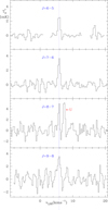 |
Fig. 1. Observed lines of the new molecule found in the 31–50 GHz domain towards TMC-1. The abscissa corresponds to the local standard of rest velocity in km s−1. Frequencies and intensities for the observed lines are given in Table 1. The ordinate is the antenna temperature corrected for atmospheric and telescope losses in mK. Spectral resolution is 38.15 kHz. Blanked channels in the top panel correspond to negative features produced in the folding of the frequency-switching observations. |
Observed line parameters for HC3S+ in the laboratory and in TMC-1.
From the line parameters in Table 1, adopting a dipole moment of 1.73 D (see Sect. 4), and assuming a uniform source with a radius of 40″ (Fossé et al. 2001), we derive a column density of N(HC3S+) = (2.0 ± 0.4)×1011 cm−2 and a rotational temperature of 10 ± 2 K. This value is compatible with the upper limit of 3 × 1011 cm−2 obtained by Cernicharo et al. (2020a) from a search based on ab initio calculations. The sensitivity improvement added by the new data has permitted its detection in TMC-1.
Protonated C2S was predicted to be abundant in cold dense clouds by Agúndez et al. (2015) based on its high proton affinity and large abundance of C2S. We therefore carried out ab initio calculations for HC2S+, which has a 3Σ ground electronic state (see also Puzzarini 2008), to search for the lines NN → N − 1N − 1 (J = N), which could be in good harmonic relation. Our estimates for B and D are 6048 MHz and 0.12 kHz, respectively. These lines should exhibit a weak hyperfine splitting of ∼0.8 MHz. Two of these lines (33–22 and 44–33) fall within our Q-band survey. However, we have not found two harmonically related features (3:4) that could be attributed to them. The explored ranges for the 33–22 and 44–33 transitions are ±40 MHz around 36 288 and 48 384 MHz, respectively. The sensitivity of our data in these ranges is ∼0.5 and ∼1 mK, respectively. The other components of each triplet (J = N ± 1) will show a more complex pattern due to the spin–spin and spin–rotation interaction. We adopted the λ parameter from C2S, which is isoelectronic with HC2S+, but the predictions have a large uncertainty and therefore a radioastronomical search is not straightforward for these transitions. Using the dipole moment derived in our ab initio calculations (2.67 D), and assuming a rotational temperature similar to that of CCS (5 K), we derive a 3σ upper limit for its column density ≤ 9×1011 cm−2. For Tr = 10 K, the 3σ upper limit is 3 × 1011 cm−2. Nevertheless, the lines searched here are not best suited for a detection of HC2S+ as they are expected to be much higher in energy that those of the J = N + 1 series, which, as mentioned above, require a good estimate of the spin–spin interaction constant, λ, to obtain reliable frequencies with which to carry out a search for this molecule.
We also derived column densities for S-bearing molecules related to HC3S+ using our Q−band line survey of TMC-1. The line parameters are given in Table A.1. For CS and HCS+ we only observed the J = 1 − 0 transition and therefore we adopted a rotational temperature of 10 K. A similar approach was taken by Vastel et al. (2018) in their study of L1544. The column density of CS, whose J = 1 − 0 line has a significant optical depth, was derived from that of C34S adopting the 32S/34S abundance ratio of 25 ± 5 determined from C3S and C3 34S. The derived column densities for all species studied in this paper are given in Table 3. The derived column densities for CCS and C3S are in good agreement with those derived by Saito et al. (1987) and Yamamoto et al. (1987). A detailed analysis of the effect of the assumed rotational temperature on diatomic or linear polyatomic molecules is provided in Appendix A.
4. Quantum chemical calculations for HC3S+
In order to obtain precise geometries and spectroscopic molecular parameters that help in the assignment of the observed lines we carried out high-level ab initio calculations for HC3S+ using the Molpro 2018.1 (Werner et al. 2018) and Gaussian09 (Frisch et al. 2013) program packages. We followed the same strategy used previously for HC3O+ (Cernicharo et al. 2020a), whereby we scaled our calculations with a molecular system that is isoelectronic to the target molecule. In the present case, we chose HC3P (see also Thorwirth et al. 2020), whose rotational parameters have been experimentally determined by Bizzocchi et al. (2001), as a reference system to scale the HC3S+ calculations. The geometry optimisation calculations were carried out at CCSD(T)-F12/cc-pCVTZ-F12 level of theory (Raghavachari et al. 1989; Adler et al. 2007; Knizia et al. 2009; Hill et al. 2010; Hill & Peterson 2010), which has proven to be a suitable method with which to accurately reproduce the molecular geometry of analogue molecules (Cernicharo et al. 2019, 2020a). We first calculated Be for HC3P and then computed B0 using the zero-point vibrational contribution calculated at MP2/cc-pVTZ level of theory. The agreement with the experimental value is very good, with a relative error of 0.02 % (see Table 2). The B0 value for HC3S+ was calculated using the Be value and the zero-point vibrational correction, obtained at CCSD(T)-F12/cc-pCVTZ-F12 and MP2/cc-pVTZ levels of theory, respectively. This value was then corrected using a scaling factor obtained from the ratio between the experimental and theoretical values derived for HC3P. The final value of B0 obtained for HC3S+ agrees very well with that obtained from observations and in the laboratory, with a relative error of around 0.01%. In addition, the centrifugal distortion value obtained using the same procedure at MP2/cc-pVTZ level of theory is compatible with that obtained from the fit of the lines. The computed dipole moment is 1.73 D. The results of our calculations are in agreement with those obtained by Thorwirth et al. (2020), which were made using the same procedure but at a different level of theory.
Theoretical and experimental values for the spectroscopic parameters of HC3S+ (all in MHz).
5. Laboratory detection of HC3S+
The rotational spectrum of HC3S+ was measured using a Balle-Flygare-type Fourier transform microwave (FTMW) spectrometer combined with a pulsed discharge nozzle (Endo et al. 1994; Cabezas et al. 2016), which was previously used to characterise other highly reactive molecules. The transient species, HC3S+, was produced in a supersonic expansion by a pulsed electric discharge of a gas mixture of C2H2 (0.2%), H2 (5%), and CS2 (0.2%) diluted in Ne and applying a voltage of 1100 V through the throat of the nozzle source. The rotational constants derived from the astronomical observations were used to predict the frequencies of the rotational transitions J = 3 − 2, 4–3, and 5–4 of HC3S+. A scan of ±2 MHz was achieved around these frequencies and three lines were observed at 16412.7583, 21883.6632, and 27354.5443 MHz with an uncertainty of 3 kHz (see Fig. 2 and Table 1), just 1–5 kHz away from the predicted frequencies using the derived rotational and distortion constants from the TMC-1 observations. The following experimental results confirm that these lines belong to a transient species: (i) they disappear in the absence of electric discharge, and (ii) the lines disappear when CS2 is removed from the gas mixture. No more lines at lower or higher frequencies (J = 2 − 1 and 6–5) could be observed due to the spectrum weakness and the poorer performance of the spectrometer at those frequencies.
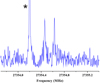 |
Fig. 2. FTMW spectra of HC3S+ showing the J = 5 − 4 rotational transition at 27.3 GHz. The spectrum was achieved by 10 000 shots of accumulation at a repetition rate of 10 Hz. The coaxial arrangement of the adiabatic expansion and the resonator axis produces an instrumental Doppler doubling. The resonance frequency is calculated as the average of the two Doppler components. The feature marked with an asterisk is an artifact. |
The fitted rotational and distortion constants derived from the laboratory data alone are given in column Exp. (labo) of Table 2. A merged fit to the laboratory and astronomical frequencies provides a rotational constant B = 2735.46311 ± 0.00023 MHz and a distortion constant D = 0.1720 ± 0.0029 kHz. The standard deviation of the fit is 5.8 kHz and the correlation coefficient between B and D is 0.82. These are the recommended constants to predict the rotational spectrum of HC3S+. The predicted frequencies, Einstein coefficients, upper energy levels, and line strengths for rotational transitions with J ≤ 30 are given in Table B.1. The observed minus calculated frequencies from this merged fit are given in Table 1.
6. Chemical model
From Table 3 we derive the following neutral-to-protonated column density ratios: CS/HCS+ = 35 ± 6, C2S/HC2S+ ≥ 60, and C3S/HC3S+ = 65 ± 20. In order to interpret these ratios we carried out chemical model calculations similar to those presented by Agúndez et al. (2015), who discussed the chemistry of protonated molecules in cold dense clouds. We have adopted the KIDA kida.uva.2014 chemical network (Wakelam et al. 2015). The abundances of sulfur-bearing molecules are strongly dependent on the depletion of sulfur, which is still a matter of debate (Vidal et al. 2017; Vastel et al. 2018). Here we have adopted the so-called set of low-metal elemental abundances (see Agúndez & Wakelam 2013), in which S/H = 8 × 10⁻⁸. The resulting fractional abundances and abundance ratios are shown in Fig. 3 as a function of time. If we focus on the so-called early time (105–106 yr), at which calculated abundances agree better with observations (e.g. Agúndez & Wakelam 2013), we see that the chemical model reproduces the observed fractional abundances of neutral and protonated molecules reasonably well, at the exception of C2S and HCS+, which translates to good agreement between calculated and observed [M]/[MH+] ratios for M = C3S but not for M = CS and C2S.
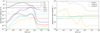 |
Fig. 3. Calculated abundances (left) and abundance ratios (right) as a function of time for a cold dense cloud. Observed values in TMC-1 (see Table 3) are indicated by horizontal dashed lines. The observed HC2S+ abundance and C2S/HC2S+ ratio are an upper and a lower limit, respectively, and are indicated by vertical arrows. Dotted lines represent the calculated abundances of C2S and HC2S+ (left panel) and its ratio (right panel) when the reaction O + C2S is neglected. |
Column densities derived for S-bearing species in TMC-1.
As discussed by Agúndez et al. (2015), in a simplified chemical scheme, a protonated molecule is formed through proton transfer from a proton donor (typically HCO+, H3O+, and  ) and destroyed by dissociative recombination with electrons. In that case, the neutral-to-protonated abundance ratio at steady state is simply given by the ratio of rate constants of the reaction of dissociative recombination and of proton transfer multiplied by the abundance ratio between electrons and the proton donor. This simple scheme should hold unless there are important alternative ion-molecule reactions of formation of the ion other than proton transfer to the neutral.
For HC3S+ the chemical model indicates that the main formation reactions are proton transfer to C3S from HCO+ and H3O+, although the reactions S+ + C3H2 (cyclic or linear) and S + C3 (cyclic or linear) are also efficient at the same level. The reactions of S+ with both cyclic and linear C3H2 have been calculated to be barrierless when leading to HC3S+ (Redondo et al. 1999). However, the cyclic isomer of C3H2 is 28 times more abundant than the linear one in TMC-1 (Fossé et al. 2001), and thus the reaction S+ + c-C3H2 will contribute significantly more than S+ + H2C3 to the formation of HC3S+. The fact that the calculated C3S/HC3S+ ratio is in agreement with the observed value supports the hypothesis that HC3S+ is formed by the aforementioned reactions.
In the case of HCS+, the chemical model underestimates its formation, which is carried out by proton transfer to CS from H3O+ and HCO+ and by the reaction between CS+ and H2. Including grain-surface chemical reactions, Vidal et al. (2017) calculate a CS/HCS+ ratio in better agreement with observations, especially at late times. The reason for the low abundance of HCS+ in our gas-phase model may be related to the underproduction of H2S (see e.g. Agúndez & Wakelam 2013), which is enhanced when including grain-surface chemistry, and which can increase the abundance of HCS+ through reactions like H2S + C+ and H2S+ + C.
While the calculated abundance of HC2S+ is in agreement with the observed upper limit, the calculated C2S/HC2S+ ratio is too low because the chemical model severely underestimates the abundance of C2S. This is because the chemical network kida.uva.2014 includes an efficient destruction channel for C2S through reaction with O atoms, based on estimations by Loison et al. (2012). If this reaction is neglected, the calculated abundance of C2S is shifted up and becomes very close to the observed value, while the abundance of HC2S+ also increases, remaining consistent with the observed upper limit (see dotted lines in Fig. 3). Accurate calculations of the rate constant of the O + C2S reaction at low temperatures are needed to shed light on the chemistry of C2S in cold dense clouds.
7. Conclusions
We report the first identification in space of protonated C3S. Four harmonically related lines observed toward TMC-1 using the Yebes 40 m radiotelescope have been unambiguously assigned to this ion thanks to accurate ab initio quantum chemical calculations and laboratory measurements of the rotational spectrum of this species. The derived C3S/HC3S+ ratio of 55 ± 20 is well reproduced by a gas-phase chemical model in which HC3S+ is mostly formed through protonation of C3S and the reactions S+ + C3H2 and S + C3 .
.
Acknowledgments
We thank Ministerio de Ciencia e Innovación of Spain (MICIU) for funding support through projects AYA2016-75066-C2-1-P, PID2019-106110GB-I00, PID2019-107115GB-C21 / AEI / 10.13039/501100011033, and PID2019-106235GB-I00. We also thank ERC for funding through grant ERC-2013-Syg-610256-NANOCOSMOS. M.A. thanks MICIU for grant RyC-2014-16277. Y.E. thanks Ministry of Science and Technology of Taiwan through grant MOST108-2113-M-009-25.
References
- Adler, T. B., Knizia, G., & Werner, H.-J. 2007, J. Chem. Phys., 127, 221106 [Google Scholar]
- Agúndez, M., & Wakelam, V. 2013, Chem. Rev., 113, 8710 [Google Scholar]
- Agúndez, M., Cernicharo, J., de Vicente, P., et al. 2015, A&A, 579, L10 [NASA ADS] [CrossRef] [EDP Sciences] [Google Scholar]
- Bizzocchi, L., Thorwirth, S., & Müller, H. S. P. 2001, J. Mol. Spectrosc., 205, 110 [Google Scholar]
- Cabezas, C., Guillemin, J.-C., & Endo, Y. 2016, J. Chem. Phys., 145, 184304 [Google Scholar]
- Cernicharo, J. 1985, Internal IRAM Report (Granada: IRAM) [Google Scholar]
- Cernicharo, J. 2012, in ECLA 2011: Proc. of the European Conference on Laboratory Astrophysics, eds. C. Stehl, C. Joblin, & L. d’Hendecourt (Cambridge: Cambridge Univ. Press), EAS Publ. Ser., 251, https://nanocosmos.iff.csic.es/?page_id=1619 [Google Scholar]
- Cernicharo, J., Guélin, M., Hein, H., & Kahane, C. 1987, A&A, 181, L9 [Google Scholar]
- Cernicharo, J., Cabezas, C., Pardo, J. R., et al. 2019, A&A, 630, L2 [NASA ADS] [CrossRef] [EDP Sciences] [Google Scholar]
- Cernicharo, J., Marcelino, N., Agúndez, M., et al. 2020a, A&A, 642, L17 [NASA ADS] [CrossRef] [EDP Sciences] [Google Scholar]
- Cernicharo, J., Marcelino, N., Pardo, J. R., et al. 2020b, A&A, 641, L9 [NASA ADS] [CrossRef] [EDP Sciences] [Google Scholar]
- Cernicharo, J., Marcelino, N., Agúndez, M., et al. 2020c, A&A, 642, L8 [NASA ADS] [CrossRef] [EDP Sciences] [Google Scholar]
- Denis-Alpizar, O., Stoecklin, T., Guilloteau, S., & Dutrey, A. 2018, MNRAS, 478, 1811 [Google Scholar]
- Endo, Y., Kohguchi, H., & Ohshima, Y. 1994, Faraday Discuss., 97, 341 [Google Scholar]
- Fossé, D., Cernicharo, J., Gerin, M., & Cox, P. 2001, ApJ, 552, 168 [Google Scholar]
- Frisch, M. J., Trucks, G. W., Schlegel, H. B., et al. 2013, Gaussian 09, Revision D.01 [Google Scholar]
- Goldsmith, P. F., & Langer, W. D. 1999, ApJ, 517, 209 [Google Scholar]
- Gordy, W., & Cook, R. L. 1984, Microwave Molecular Spectra, Chapter V (New York: Wiley) [Google Scholar]
- Hill, J. G., & Peterson, K. A. 2010, Phys. Chem. Chem. Phys., 12, 10460 [Google Scholar]
- Hill, J. G., Mazumder, S., & Peterson, K. A. 2010, J. Chem. Phys., 132, 054108 [Google Scholar]
- Hirahara, Y., Ohshima, Y., & Endo, Y. 1994, J. Chem. Phys., 101, 7342 [Google Scholar]
- Hunter, E. P. L., & Lias, S. G. 1998, J. Phys. Chem. Ref. Data, 27, 413 [Google Scholar]
- Kaifu, N., Ohishi, M., Kawaguchi, K., et al. 2004, PASJ, 56, 69 [Google Scholar]
- Kawaguchi, K., Kasai, Y., Ishikawa, S.-I., et al. 1994, ApJ, 420, L95 [Google Scholar]
- Knizia, G., Adler, T. B., & Werner, H.-J. 2009, J. Chem. Phys., 130, 054104 [Google Scholar]
- Loison, J.-C., Halvick, P., Bergeat, A., et al. 2012, MNRAS, 421, 1476 [Google Scholar]
- Marcelino, N., Agúndez, M., Tercero, B., et al. 2020, A&A, 643, L6 [NASA ADS] [CrossRef] [EDP Sciences] [Google Scholar]
- Müller, H. S. P., Schlöder, F., Stutzki, J., & Winnewisser, G. 2005, J. Mol. Struct., 742, 215 [Google Scholar]
- Pardo, J. R., Cernicharo, J., & Serabyn, E. 2001, IEEE Trans. Antennas Propag., 49, 12 [Google Scholar]
- Pickett, H. M., Poynter, R. L., Cohen, E. A., et al. 1998, J. Quant. Spectrosc. Radiat. Trans., 60, 883 [Google Scholar]
- Puzzarini, C. 2008, Chem. Phys., 346, 45 [Google Scholar]
- Raghavachari, K., Trucks, G. W., Pople, J. A., & Head-Gordon, M. 1989, Chem. Phys. Lett., 157, 479 [Google Scholar]
- Redondo, P., Calleja, E., Barrientos, C., & Largo, A. 1999, J. Phys. Chem. A, 103, 9125 [Google Scholar]
- Saito, S., Kawaguchi, K., Yamamoto, S., et al. 1987, ApJ, 317, L1156 [Google Scholar]
- Tercero, F., López-Pérez, J. A., Gallego, J. D., et al. 2021, A&A, 645, A37 [EDP Sciences] [Google Scholar]
- Thorwirth, S., Harding, M. E., Asvany, O., et al. 2020, Mol. Phys., 118, e1776409 [Google Scholar]
- Vastel, C., Quénard, D., Le Gal, R., et al. 2018, MNRAS, 478, 5514 [Google Scholar]
- Vidal, T. H. G., Loison, J.-C., Jaziri, A. Y., et al. 2017, MNRAS, 469, 435 [Google Scholar]
- Yamamoto, S., Saito, S., Kawaguchi, K., et al. 1987, ApJ, 317, L119 [Google Scholar]
- Wakelam, V., Loison, J.-C., Herbst, E., et al. 2015, ApJS, 217, 20 [Google Scholar]
- Werner, H. J., Knowles, P. J., Knizia, G., et al. 2018, MOLPRO, version 2018.1 [Google Scholar]
Appendix A: Column densities under LTE for linear molecules
The determination of column densities from the observed line paramaters of the rotational transitions of a molecule requires knowledge of the collisional rates of the molecular species under study. These values are not always available and rotational diagrams are used to derived rotational temperatures, Tr, and column densities (Goldsmith & Langer 1999). Often only one line has been observed and therefore an assumption has to be made as to the rotational temperature. The line parameters of the species studied in this paper are given in Table A.1.
Observed line parameters in TMC-1 for CS, HCS+, C2S and C3S.
In this section we analyse how the derived column density depends on the adopted Tr for a range of frequencies and upper energy levels. Let us assume an optically thin line (τ ≪ 1) with frequency νul and arising from an upper level with energy Eu. If the medium has uniform excitation conditions, and the molecular levels are populated under a uniform rotational temperature Tr, then, the observed brightness temperature (TB) is given by:
 (A.1)
(A.1)
where Tbg is the temperature of the cosmic radiation background, and τ(v) the opacity of the line at frequency ν, which is given by
 (A.2)
(A.2)
where Nl, Nu, gl, and gu are the column densities and statistical weights of the lower and upper levels, Aul is the Einstein coefficient of the transition, and ϕ(ν) is the normalised line profile, which for a Gaussian line is given by
 (A.3)
(A.3)
where  ), with Δν being the line full width at half intensity (in km s−1). Using the following relations in which Sul is the line strength and μ is the permanent dipole moment of the molecule,
 (A.4)
(A.4)
 (A.5)
(A.5)
 (A.6)
(A.6)
we derive
 (A.7)
(A.7)
where N is the column density of the molecule, Qrot is the rotational partition function, h is the Planck constant, and kB is the Boltzmann constant. For linear molecules, the rotational partition function (Gordy & Cook 1984) is given by:
 (A.8)
(A.8)
where B is the rotational constant of the molecule. This approximation is rather accurate, even for low values of Tr if Tr/B≫1. Hence, the brightness temperature at the line centre (ν = νul) is given by
 (A.9)
(A.9)
and the column density can be derived from the observed brightness temperature of the observed transition from the following expression:
 (A.10)
where C is a constant that depends on the molecular parameters and is given by
 (A.11)
in these expressions Δv is in km s−1, and corresponds to the line full width at half power intensity (see expression (A.3)), B is in GHz and μ in D.
The function f depends on Eu, νul, and Tr as
 (A.12)
and it shows a smooth behaviour with Tr for most cases of interest in the frequency range of our survey. Figure A.1 shows the value of the function f for different values of the energy of the upper level and for a frequency of 42.674 GHz (the frequency of the J = 1 − 0 transition of HCS+). The case Eu = 2 K corresponds, specifically, to the J = 1 − 0 transition of HCS+. For this particular case the value of f for Tr = 5 K is 6.59 while for Tr = 10 K it is 7.56. Hence, assuming Tr = 10 K represents a change in the column density of +15% with respect the case with Tr = 5 K. The bottom panel of Fig. A.1 shows the function f normalised to its value at Tr = 10 K. Hence, the different plots, which correspond to different energies of the upper level (always for a frequency of 42.674 GHz), show the relative error on the estimated column density assuming Tr = 10 K with respect other values of the rotational temperature.
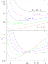 |
Fig. A.1. Dependency of the derived column density on the assumed rotational temperature for a line at 42.674 GHz (HCS+J = 1 − 0; upper panel). The upper energy level is varied between 2 and 10 K. Lower panel: same function but normalised to its value for Tr = 10 K. |
For most molecules detected in the survey we observe transitions with low Ju and therefore with moderate upper energy levels. The error on the derived column density from the observed line parameters of just one transition of a linear molecule is below 20% for Eu ≤ 6 K and for Tr between 5 and 10 K. This applies particularly to CS and HCS+ and other linear species in our survey. For transitions involving levels with Eu ≫ Tr the error on the estimated column density can be considerably larger. From Fig. A.1 we can see that a change from Tr = 6 to 10 K introduces an error of ∼1.5 for a transition with Eu = 10 K. The error can reach a factor three if Eu = 15 K. For these cases a realistic estimation of the rotational temperature is needed based on the observation of several rotational transitions of the molecule under study.
An additional source of uncertainty in the column density when only one line is observed is the assumption of local thermodynamical equilibrium (LTE) under a uniform rotational temperature for all rotational levels. For the physical conditions of TMC-1, TK = 10 K and n(H2) = 4 × 104 cm−3 (Cernicharo et al. 1987; Fossé et al. 2001), the J = 1 − 0 line of most molecules will have an excitation temperature close to the kinetic one. However, the excitation of rotational levels with higher values of J will be certainly below the kinetic temperature. To quantify this effect we used the Large Velocity Gradient (LVG) approximation for CS. We assumed a line width of 0.6 km −1 and a column density of 1012 cm−2 (optically thin case). We adopted the collisional rates CS/p-H2 provided by Denis-Alpizar et al. (2018). We obtain Tex(J = 1 − 0) = 7.3 K and Tex(J = 2 − 1) = 3.9 K. If the collisional rates CS/o-H2 from the same authors are adopted, then the derived excitation temperatures for these transitions are 8.9 and 4.9 K, respectively. From the observed line parameters of the J = 1 − 0 transition of C34S and 13C34S given in Table A.1, we derive N(C34S) = 6.5 × 1012 cm−2, and N(13C34S) = 5.5 × 1010 cm−2. These values are a factor 2.2 and 2.6 lower than those provided in Table 3, respectively, which have been obtained assuming a uniform rotational temperature of 10 K. Hence, the main source of uncertainty in the derived column densities could be related to the assumption of a uniform rotational temperature for all rotational levels of a linear molecule (LTE conditions), rather than to the adopted rotational temperature.
Appendix B: Observed line parameters and frequency predictions up to J = 30
The observed line parameters for the sulfur-bearing molecules discussed in this paper are given in Table A.1. For HC3S+ they are given in Table 1. Frequency predictions for HC3S+ up to J = 30 are given in Table B.1
Predicted line frequencies for HC3S+.
All Tables
Theoretical and experimental values for the spectroscopic parameters of HC3S+ (all in MHz).
All Figures
|
Fig. 1. Observed lines of the new molecule found in the 31–50 GHz domain towards TMC-1. The abscissa corresponds to the local standard of rest velocity in km s−1. Frequencies and intensities for the observed lines are given in Table 1. The ordinate is the antenna temperature corrected for atmospheric and telescope losses in mK. Spectral resolution is 38.15 kHz. Blanked channels in the top panel correspond to negative features produced in the folding of the frequency-switching observations. |
| In the text | |
|
Fig. 2. FTMW spectra of HC3S+ showing the J = 5 − 4 rotational transition at 27.3 GHz. The spectrum was achieved by 10 000 shots of accumulation at a repetition rate of 10 Hz. The coaxial arrangement of the adiabatic expansion and the resonator axis produces an instrumental Doppler doubling. The resonance frequency is calculated as the average of the two Doppler components. The feature marked with an asterisk is an artifact. |
| In the text | |
|
Fig. 3. Calculated abundances (left) and abundance ratios (right) as a function of time for a cold dense cloud. Observed values in TMC-1 (see Table 3) are indicated by horizontal dashed lines. The observed HC2S+ abundance and C2S/HC2S+ ratio are an upper and a lower limit, respectively, and are indicated by vertical arrows. Dotted lines represent the calculated abundances of C2S and HC2S+ (left panel) and its ratio (right panel) when the reaction O + C2S is neglected. |
| In the text | |
|
Fig. A.1. Dependency of the derived column density on the assumed rotational temperature for a line at 42.674 GHz (HCS+J = 1 − 0; upper panel). The upper energy level is varied between 2 and 10 K. Lower panel: same function but normalised to its value for Tr = 10 K. |
| In the text | |
Current usage metrics show cumulative count of Article Views (full-text article views including HTML views, PDF and ePub downloads, according to the available data) and Abstracts Views on Vision4Press platform.
Data correspond to usage on the plateform after 2015. The current usage metrics is available 48-96 hours after online publication and is updated daily on week days.
Initial download of the metrics may take a while.