| Issue |
A&A
Volume 646, February 2021
|
|
|---|---|---|
| Article Number | A117 | |
| Number of page(s) | 8 | |
| Section | Stellar structure and evolution | |
| DOI | https://doi.org/10.1051/0004-6361/202039774 | |
| Published online | 17 February 2021 | |
Strongly pulsed thermal X-rays from a single extended hot spot on PSR J2021+4026
1
INAF, Istituto di Astrofisica Spaziale e Fisica Cosmica Milano, Via A. Corti 12, 20133 Milano, Italy
e-mail: This email address is being protected from spambots. You need JavaScript enabled to view it.
2
Dipartimento di Matematica e Fisica, Università di Roma Tre, Via della Vasca Navale 84, 00146 Roma, Italy
3
Dipartimento di Fisica e Astronomia, Università di Padova, Via F. Marzolo 8, 35131 Padova, Italy
4
MSSL-UCL, Holmbury St. Mary, Dorking, Surrey RH5 6NT, UK
Received:
27
October
2020
Accepted:
8
December
2020
Abstract
The radio-quiet pulsar PSR J2021+4026 is mostly known because it is the only rotation-powered pulsar that shows variability in its γ-ray emission. Using XMM-Newton archival data, we first confirmed that its flux is steady in the X-ray band, and then we showed that both the spectral and timing X-ray properties, that is to say the narrow pulse profile, the high pulsed fraction of 80–90%, and its dependence on the energy, can be better reproduced using a magnetized atmosphere model instead of simply a blackbody model. With a maximum likelihood analysis in the energy-phase space, we inferred that the pulsar has, in correspondence of one magnetic pole, a hot spot with a temperature of T ∼ 1 MK and colatitude extension of θ ∼ 20°. For the pulsar distance of 1.5 kpc, this corresponds to a cap of R ∼ 5 − 6 km, which is greater than the standard dimension of the dipolar polar caps. The large pulsed fraction further argues against emission from the entire star surface, as it would be expected in the case of secular cooling. An unpulsed (≲40% pulsed fraction), nonthermal component, probably originating in a wind nebula, is also detected. The pulsar geometry derived with our spectral fits in the X-ray is relatively well constrained (χ = 90° and ξ = 20°–25°) and consistent with what is deduced from γ-ray observations, provided that only one of the two hemispheres is active. The evidence for an extended hot spot in PSR J2021+4026, which was also found in other pulsars of a similar age but not in older objects, suggests a possible age dependence of the emitting size of thermal X-rays.
Key words: pulsars: general / pulsars: individual: PSR J2021+4026 / stars: neutron / X-rays: stars
© ESO 2021
1. Introduction
Many isolated neutron stars with characteristic ages τ = P/2 Ṗ in the 104–107 year range show thermal X-ray emission that cannot result from their internal cooling. This is deduced from the small size of their emission regions and/or from their temperatures, which are inconsistent with those predicted by neutron star cooling theories (see e.g., Potekhin et al. 2020, and references therein). Such thermal emission is instead attributed to the external heating of small regions of the star surface, typically the polar caps. In fact, a fraction of the charges that flow in the magnetosphere are accelerated backward toward the star surface, thus heating it in localized regions and producing observable “hot spots” (Arons & Scharlemann 1979; Harding & Muslimov 2001, 2002; Cheng et al. 1986a,b; Chiang & Romani 1994). The study of this emission is often complicated by the presence of other spectral components: nonthermal X-rays from the magnetosphere or from spatially unresolved nebulae and thermal emission caused by the cooling of the rest of the surface, as in middle aged pulsars (τ ∼ 104 − 105 years), such as the “three Musketeers” (De Luca et al. 2005). When a pulsar is sufficiently old (τ ≳ 106 years) and the surface has cooled down enough, the externally-heated polar cap emission can be the only observable thermal component, as in PSR J0108−1431 (Arumugasamy & Mitra 2019), PSR B0943+10 (Rigoselli et al. 2019), and PSR B1929+10 (Misanovic et al. 2008). The X-ray emission from hot spots can appear significantly pulsed if the pulsar geometry and our line of sight (LOS) are favorable. Information on angles χ and ξ that the rotation axis makes with our LOS and with the magnetic axis, respectively, have traditionally been derived from the properties of radio emission. More recently, constraints on the pulsar geometry have also been obtained by modeling the light curves at γ-ray (Romani & Watters 2010) and, in a few cases, X-ray energies (e.g., Miller et al. 2019; Riley et al. 2019). Independent estimates of the geometrical angles will come from X-ray polarimetry (see e.g., Taverna et al. 2014, 2020) thanks to the forthcoming missions IXPE (Weisskopf et al. 2013) and eXTP (Zhang et al. 2019). These are, in fact, the only possibilities when radio emission is not seen, as in the radio-quiet rotation-powered pulsars (about 5% of those with 104 < τ < 107 years) and in other classes of objects such as the X-ray-dim isolated neutron stars (XDINSs, Kaplan et al. 2008; Turolla 2009) and the central compact objects (CCOs, De Luca 2017).
Among radio-quiet pulsars, PSR J2021+4026 is of particular interest because it is the only one that exhibited flux variations at γ-rays energies. In October 2011, Fermi-LAT observed a sudden flux drop at E > 100 MeV, occurring over a timescale of less than one week (Allafort et al. 2013). This was accompanied by a significant increase in the spin-down rate (see the timing parameters in Table 1). The frequency derivative discontinuity resembles a glitch; however, the behavior seen in PSR J2021+4026 differs from that of normal glitches (Espinoza et al. 2011; Pletsch et al. 2012) because these are usually not associated with a flux change. Furthermore, glitches are typically followed by a rapid recovery in the timing parameters, while this was not detected for PSR J2021+4026 until 2014 December (Zhao et al. 2017). More recently, in 2018 February, PSR J2021+4026 entered into a low γ-ray state again, with a Ṗ behavior similar to the one that followed the 2011 event (Takata et al. 2020).
Observed and derived parameters for PSR J2021+4026
PSR J2021+4026 has been associated to the shell-like γ-Cygni supernova remnant (SNR), SNR G78.2+2.1 (Green 2009). Its radio and X-ray shells have a size of ∼1° (Leahy et al. 2013) and a shock velocity of ∼800 km s−1 (Uchiyama et al. 2002). These values, together with the SNR distance of 1.5 ± 0.5 kpc (Landecker et al. 1980), imply an adiabatic age of 6.6 kyr, which is in agreement with the age deduced from the optical observations (Mavromatakis 2003). Thus, the age of SNR G78.2+2.1 is about one order of magnitude smaller than the spin-down age of PSR J2021+4026 (τc ∼ 75 kyr). However, this discrepancy is not uncommon in middle-aged neutron stars (see e.g., the pulsars PSR J0538+2817, Ng et al. 2007, and PSR J0855−4644, Allen et al. 2015; the XDINS RX J1856.5−3754, Mignani et al. 2013; and the “low-B” magnetar SGR 0418+5729, Turolla et al. 2011). The mismatch between the true and characteristic age can be explained if the star magnetic field substantially decayed or if the spin period at birth was close to the present one.
In the X-ray band, PSR J2021+4026 was frequently observed by Chandra and XMM-Newton. Its X-ray spectrum shows a mixture of nonthermal and thermal emission: The nonthermal component, which is apparently nonpulsed, is probably due to the pulsar wind nebula (PWN) that is spatially resolved by Chandra (Hui et al. 2015); the thermal component is instead strongly pulsed (90–100%) with a nearly sinusoidal profile. Wang et al. (2018) analyze two long XMM-Newton observations; one was obtained after the 2011 drop in the γ-ray flux and the other was obtained in the post-relaxation state in 2015. They could not find any significant change in the X-ray flux, spectrum, or pulse profile, but they noticed that the sensitivity of the current data is not sufficient to detect the small flux change (∼4%) expected from the observed Ṗ variation.
The thermal component in the spectrum of PSR J2021+4026, when fitted with a blackbody model, yields an emitting region with a size consistent with the dimensions of the polar cap in the dipole approximation,  m (Hui et al. 2015; Wang et al. 2018). Given the viewing angle of χ ∼ 90° inferred by the γ-ray data (Trepl et al. 2010), the two polar caps are visible. If both contributed to the X-ray emission, then the pulse profile would be far less pulsed (≲25%) and, for several values of ξ, it would have two peaks (e.g., Beloborodov 2002). Hui et al. (2015) conclude that the strongly pulsed and single-peaked profile implies that only one of the two polar caps is active in X-rays.
Here we present a reanalysis of the XMM-Newton data aimed to quantitatively reproduce the timing and the spectral features of PSR J2021+4026, which fit its phase-resolved spectrum with magnetized atmosphere models. In our spectral models, which were specifically computed for this pulsar, the emitting region does not have to be point-like and the cap’s semi-opening angle θcap can take any value from 0° to 90°. The temperature and the magnetic field at each latitude are consistently evaluated considering a dipolar magnetic field.
The paper is organized as follows. In Sect. 2 we briefly describe our computation of the magnetized atmosphere models, and we illustrate the approach we used to compute the phase-dependent spectrum emitted by the pulsar. We then describe the data analysis (Sect. 3) and apply our model to the observed phase-averaged and phase-resolved spectra (Sect. 4.1), and to the pulse profiles (Sect. 4.2). The results are discussed in Sect. 5.
2. Modeling the X-ray pulse profiles and spectra
Our computation of the phase-dependent spectrum emitted by a neutron star, as seen by a distant observer, is done in the following four steps by: (i) defining the stellar parameters (mass and radius, temperature and magnetic field, and geometry of the pulsar); (ii) evaluating the local spectrum emitted by each patch of the surface; (iii) collecting the contributions of all surface elements that are in view at different rotation phases, accounting for general relativistic effects, such as redshift and light bending; and (iv) convolving the observed flux at infinity with the instrumental response matrix in order to perform a spectral and timing analysis.
We adopted realistic values of mass M = 1.36 M⊙ and radius R = 13 km, which are consistent with the most recent equation of states (EOSs, see e.g., Lattimer & Prakash 2016 and references therein) and give a gravitational redshift factor of z ∼ 0.2. We computed the model atmosphere at ten different values of the colatitude (equally spaced in μ = cos θ so that they have the same area), assuming a dipole magnetic field and the ensuing temperature distribution (Greenstein & Hartke 1983). We considered models with two values for the magnetic field and temperature at the poles: [Tp = 1 MK, Bp = 4 × 10¹² G] and [Tp = 0.5 MK, Bp = 3 × 10¹² G]. The geometrical angles, χ and ξ, that the LOS and the dipole axis make with the rotation axis, respectively, were sampled by means of a 19 × 19 equally-spaced grid ranging from 0° to 90° each.
The atmospheric structure and radiative transfer were computed using the code developed by Lloyd (2003, see also Lloyd et al. 2003; Zane & Turolla 2006; González Caniulef et al. 2016), which applies the complete linearization technique to the case of a semi-infinite, plane-parallel atmosphere in radiative equilibrium. Radiation transfer calculations were performed accounting for strong magnetic fields, solving the radiative transfer equation for photons polarized both in the ordinary (O) and in the extraordinary (X) modes, with an electric field oscillating either parallel or perpendicular to the plane made by the photon propagation direction and the local magnetic field, respectively (Ginzburg 1970; Mészáros 1992). Opacities were evaluated while accounting for magnetic effects. Although the code can be generalized to mixed hydrogen-helium compositions and extended to the case of partial ionization, for the sake of simplicity here, we solely focus on a pure-hydrogen, fully ionized atmospheric slab. Each run requires the intensity B of the local magnetic field and the angle θB it forms with the local slab normal, the effective temperature T, and the surface gravity g as input. For this reason, we divided the atmospheric layer into a number of plane-parallel patches, infinitely extended in the transverse direction and emitting a total flux σT4. The code returns, in output, the intensities IO and IX of the emerging O- and X-mode photons as functions of the energy E and the two polar angles θk and ϕk, which identify the photon direction k with respect to the local normal. These angles can be written as functions of the two viewing angles χ and ξ and of the so-called impact angle η, which provides the inclination of the magnetic axis with respect to the LOS at each rotational phase γ = Ωt:
 (1)
(1)
(see e.g., Taverna et al. 2015; González Caniulef et al. 2016).
The radiation transfer equation was solved for 20 photon energies uniformly distributed on a logarithmic scale from 0.1 to 10 keV, for ten values of α = cos θB, 15 values of μk = cos θk, and five values of ϕk, which are all linearly spaced. The southern hemisphere was built by exploiting the symmetry properties of the opacities: μk = −μk, ϕk = π − ϕk.
Once the emerging flux at each patch was known, the spectrum at infinity was computed by collecting all the contributions that are in view at a certain rotational phase γ, accounting for general relativistic effects. Since we are interested in radiation emerging from polar caps which are not necessarily point-like, we considered semi-opening angles θcap of 5° (which can still be treated as point-like), 10, 20, 30, 45, 65, and 90° (the whole hemisphere). The observed flux was stored in a seven-dimensional array F∞ (E, γ, Bp, Tp, θcap, ξ, χ), which associates the (discrete) values of the energy- and phase-dependent intensity at each set of parameters.
The final step of the computation consisted in convolving the array F∞ with the instrumental response in order to properly compare the model with the observed data. This is described in the next section.
3. Observations and data analysis
We analyzed the two longest XMM-Newton observations of PSR J2021+4026, which were obtained in 2012 April (Obs. ID 0670590101) and in 2015 December (Obs. ID 0763850101) in the low γ-ray and in the post-relaxation states, respectively (see Table 2). The MOS1/2 cameras were operated in full-window mode with a medium and thick optical filter, while the pn camera was in small-window mode with a medium filter. Only the pn time resolution (5.7 ms with respect to 2.6 s of the MOS cameras) is adequate to reveal the pulsations of the source.
Exposure times and source counts for PSR J2021+4026 in the three EPIC cameras.
The data reduction was performed using the EPPROC and EMPROC pipelines of version 15 of the Science Analysis System (SAS). We selected single- and multiple-pixel events (PATTERN≤4 and ≤12) for both the pn and MOS1/2. We then removed time intervals of a high background using the SAS program ESPFILT with standard parameters. The resulting net exposure times and counts are summarized in Table 2.
Throughout the entire timing analysis, we folded the data at the periods derived from the known pulsar ephemeris appropriate for each observing epoch (Table 1), after correcting the time of arrivals to the Solar System barycenter with the tool BARYCEN.
3.1. Maximum likelihood spectral extraction
To extract the source counts and spectra, we used a maximum likelihood (ML) technique, as implemented by Rigoselli & Mereghetti (2018) and Rigoselli et al. (2019). In short, this consists in estimating the most probable number of source and background counts that reproduce the observed data, assuming that source events are spatially distributed according to the instrumental point-spread function (PSF), while the background events are uniformly distributed. The expectation value of total counts in the image pixel (i, j) is
 (2)
(2)
where b gives the background in counts per unit area (cts asec−2), s is the total number of source counts, and PSFij is the normalized point-spread function corresponding to that pixel. We take the PSF dependence on photon energy and the position on the detector into account, as derived from in-flight calibrations (Ghizzardi 2002). The ML method has the advantage of exploiting all the source events that are located in the region of interest and being compatible with the PSF. Furthermore, the background is determined locally, and not in a different region of the detector.
The above ML method, which is referred to as “2D-ML” from this point on, can be generalized to also take the pulse phase information of the events for periodic sources into account (“3D-ML”, Hermsen et al. 2013). If the events are binned in spatial and phase coordinates, a tridimensional space is defined, where the expectation value of the bin (i, j, k) is
 (3)
(3)
Now su and sp represent the source counts for the unpulsed and pulsed components, respectively, while fk is the normalized pulse profile at phase φk. In this work, to describe the pulse shape, we considered a sine function
 (4)
(4)
and a Gaussian function
![Mathematical equation: $$ \begin{aligned} f_k=\frac{1}{\sqrt{2\pi \sigma _\varphi ^2}}\exp {\left[-\frac{(\varphi _k-\varphi _0)^2}{2\sigma _\varphi ^2} \right]}, \end{aligned} $$](/articles/aa/full_html/2021/02/aa39774-20/aa39774-20-eq9.gif) (5)
(5)
where φ0 is the absolute phase and σφ is the characteristic Gaussian width.
The maximum likelihood ratio (MLR), which is defined as the difference between the likelihood of the assumed model with its best parameters and that of the null hypothesis, is used to evaluate the significance of the results. In the case of 2D-ML, the MLR compares the likelihood of having a point source with respect to having only a background; whereas in the case of 3D-ML, it is obtained as a comparison between the likelihood of having a pulsating source with respect to the likelihood of having a source with constant emission. The significance in σ of the detection is the square root of the MLR.
Source spectra can be extracted by applying the ML to the images in different energy bins and using the appropriate PSF for each one. If we use Eq. (2) with the whole dataset, we get the phase-averaged spectrum, while if we divide the data into phase bins, we get the phase-resolved spectra. We note that all the spectra derived in this way contain the contributions of both the pulsed and unpulsed emission. Conversely, using the 3D-ML (Eq. (3)), we can obtain distinct spectra for the pulsed and unpulsed emission. In this context, the pulsed fraction (PF) is defined as the ratio between the pulsed and the total counts, as a function of the energy:
 (6)
(6)
We applied the ML analysis in a circular region centered at RA =  , Dec =
  with a radius of 40″, in order to account for the different fields of view of each observation and camera. We first extracted the pulse profile dividing the data set into ten phase bins. Then, considering that the folded light curves are symmetric around phase 0.5 and also that the atmosphere model has the same symmetry, we summed the corresponding spectra two by two to obtain the five phase ranges highlighted in the inset of Fig. 1.
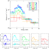 |
Fig. 1. Phase-resolved spectrum of PSR J2021+4026 fitted with a power law (Γ = 1.0) and the atmosphere model discussed in Sect. 2 (Tp = 1 MK, Bp = 4 × 10¹² G, θcap = 20°, χ = 90°, ξ = 25°). Main panel: spectra corresponding to the five phase bins displayed in the inset. Bottom panels: five spectra and their residuals, in units of σ, with respect to the best fit (same color code as before). The lines indicate the two spectral components: The thermal one changes with phase, while the power law is constant. |
3.2. Spectral fitting
We performed the spectral fits using XSPEC (version 12.11.0) and the photoelectric absorption model TBABS, with cross sections and abundances from Wilms et al. (2000). The spectra of the three cameras were fitted simultaneously, including a normalization factor to account for possible cross-calibration uncertainties. All the spectra were grouped to achieve at least 100 (phase-averaged spectra) or 50 counts (phase-resolved as well as unpulsed and pulsed spectra) in each energy bin. We give all the errors at a 1σ confidence level.
Phase-resolved spectroscopy is usually performed by independently fitting the spectra corresponding to different phase intervals and examining how the derived best-fit parameters change as a function of the phase. In our analysis we followed a different approach based on global fits in the energy-phase space. In fact, by proper integration of the array F∞ described in Sect. 2 over E and γ, we can obtain the model flux in each energy and phase bin. This model is fitted simultaneously to the phase-resolved spectra to derive a single set of the best-fit parameters Bp, Tp, θcap, ξ, χ.
4. Results
We first applied the ML to the two single observations and we found no significant variations between the two epochs: The count rate measured by the pn camera is 0.0122 ± 0.0006 cts s−1 in 2012 and 0.0125 ± 0.0006 cts s−1 in 2015, which is a difference of 2.4 ± 6.8%. We can thus set a 3σ upper limit of 22.8% on the long-term variability. The count rate measured by the MOS cameras are different in the two observations (see Table 2), but this is due to the different setting of the instruments in the two epochs. Therefore, in the following, we present the results obtained by summing the data of the two observations1.
4.1. 2D-ML spectral analysis
We first modeled the phase-averaged spectrum of PSR J2021+4026 using a power law plus a blackbody, and we found that this model fits the data well, with a reduced  for 32 degrees of freedom (d.o.f.) and a null-hypothesis probability (nhp) of 0.78. The best-fitting photon index Γ = 1.2 ± 0.2, observed temperature kT∞ = 0.221 ± 0.015 keV, and emitting radius
  m (evaluated for d = 1.5 kpc) are in excellent agreement with what was found in previous works (Hui et al. 2015; Wang et al. 2018). For this model, the column absorption is
  cm−2.
cm−2.
We then fit the spectrum with some of the magnetized hydrogen atmosphere models available in XSPEC. In particular, the NSMAXG models (Ho et al. 2008, 2014) allow one to specify if the magnetic field and the temperature are constant on the surface, or if they follow the profile expected for a dipole field. As summarized in the first part of Table 3, all of these models give a good fit if they are combined with an absorbed power law with Γ ∼ 1.1 and NH ∼ 9 × 1021 cm−2. The effective temperature is about 0.66 MK or 1 MK, depending on whether the impact angle η (see Eq. (1)) is 0° or 90°, respectively. The corresponding emitting radii Rem of  km or
km or  km indicate that the thermal emission comes from a very large region or even from the whole surface; in fact, if we fix Rem = R = 13 km, we still obtain a good fit.
Spectral results.
To further investigate the possible emission from the whole surface, we added a second thermal component with a temperature Tcool and an emitting radius fixed to that of the star to the best-fitting spectrum. We let Tcool free to vary, but the resulting best-fitting value was not constrained. In the case of blackbody models, we found Tcool < 84 eV with  for 31 d.o.f. (corresponding to an F-test probability of 0.02 compared to the single-blackbody model). We repeated the analysis with the NSMAXG models and found Tcool < 63 eV, with
  for 31 d.o.f. (F-test probability of 0.85). These results indicate that the addition of a thermal component from the whole surface is not statistically required and we derived a 3σ upper limit of its luminosity in the range (5 − 16) × 1032 erg s−1 (depending on the thermal model used).
Finally, we used our magnetized atmosphere models presented in Sect. 2 and we found that only the model with Teff = 1 MK gives an acceptable  (0.96 for 33 d.o.f. with respect to 3.8 of the model with Teff = 0.5 MK). All the explored χ and ξ angles gave equally good results for best fit emitting regions with θcap ∼ 20°, which corresponds to a radius of about 5−6 km. The addition of an absorbed power law with Γ = 1.0 ± 0.2 and NH = (8.5 ± 0.4) × 1021 cm−2 is also required in these cases.
To constrain the pulsar geometry, we had to rely on the phase-resolved spectroscopy: We fit the five phase-resolved spectra of PSR J2021+4026 with our models for all the geometries and we got good fits ( ) for a restricted set of angles: 100° ≲χ + ξ ≲ 120°. Moreover, as previous works have already noticed, it is impossible to reproduce the observed data if X-rays are emitted by both hemispheres. The best fit is obtained when χ = 90° and ξ = 25°, with approximately the same spectral parameters found in the phase-averaged spectral analysis, see Table 3. We remark that with our fitting method, the normalization of the atmosphere models is linked for all the phases and it leads to Rem = 5.1 ± 0.2 km or Rem = 5.5 ± 0.2 km, depending on which of the two hemispheres is active. These results were obtained including a power law with a constant flux at all phases, which is consistent with the assumption that the nonthermal component is entirely unpulsed.
4.2. 3D-ML timing and spectral analysis
The 3D-ML analysis allows us to simultaneously exploit, in a very effective way, the combined timing and spectral information. The pulsations of PSR J2021+4026 are detected with the highest significance in the 0.7 − 3 keV energy range. In applying the 3D-ML analysis in this range with ten phase bins, we found that the pulse profile is better described by a Gaussian (MLRgauss = 245) than by a sine function (MLRsine = 227), as it is shown in the left panel of Fig. 2. The use of a Gaussian thus gives an improvement of the MLR of 18, corresponding to a significance greater than 4σ.
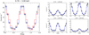 |
Fig. 2. Phase-folded light curves of PSR J2021+4026 as observed by EPIC-pn in the range of 0.7 − 3 keV (left panel) and 0.7 − 1 − 1.45 − 2 − 3 keV (right panel). The data (black dots) were obtained with the 2D-ML in ten phase bins. The red (sine, Eq. (4)) and blue (Gaussian, Eq. (5)) lines were obtained with the 3D-ML. |
The Gaussian has a phase width σφ = 0.15 ± 0.01, and PF = 0.77 ± 0.05 (defined as in Eq. (6)). In the softer energy range (0.4 − 0.7 keV), we found hints for pulsations with PF = 0.48 ± 0.26 at a 1.5σ level, while above 3 keV no pulsations are detected.In fact, the source has s = 288 ± 28 counts above 3 keV, corresponding to a detection at more than 10σ, but only  of these counts are pulsed, yielding a 3σ upper limit PF < 0.34. Then, we divided the central energy range into four bins (0.7 − 1 − 1.45 − 2 − 3 keV) and we applied the 3D-ML analysis to each pulse profile with a Gaussian σφ fixed at 0.15. The data and the corresponding best fits are shown in the right panel of Fig. 2. The measured su(E) and sp(E) were used to derive the unpulsed and the pulsed spectra, respectively, and the PF as a function of energy (see Fig. 3).
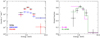 |
Fig. 3. Total, unpulsed, and pulsed spectra (left panel) and corresponding PF (right panel) of PSR J2021+4026 as observed by EPIC-pn and extracted with the 3D-ML, assuming a Gaussian function (Eq. (5)) for the pulse profile. The solid lines represent the PF computed in the case of a power law plus a blackbody (PL+BB, magenta line), and a power law plus a magnetized atmosphere (PL+ATMO, green line). |
We fit the unpulsed and pulsed spectra with our models, with the respective normalizations correctly evaluated as explained in Sect. 2. Differently from what we did in the previous section, now we can be more lenient with the assumption that the power law has a constant flux, and we can investigate its contribution to the pulsed spectrum simply by adding a power law model with free normalization to each spectrum. We found that the best-fitting geometry is χ = 90° and ξ = 20°, and that the unpulsed power law has a normalization consistent with 0, independently of which of the two hemispheres is emitting. We obtained  and 1.09 for 9 d.o.f., respectively, and spectral parameters very similar to those found with phase-resolved spectroscopy. We also tested the power-law plus blackbody model, adopting the same hypothesis that both the unpulsed and pulsed spectra could show a mixture of thermal and nonthermal emission. We found a worse best fit, with
  for 7 d.o.f. Also, in this case, the power law is entirely unpulsed, while the blackbody contributes to both the unpulsed and pulsed spectra.
Using the best-fit parameters of all the models summarized in the last part of Table 3, we computed the expected PF as a function of energy, which is shown in the right panel of Fig. 3. Above 3 keV, the observed emission is entirely due to the nonthermal photons. The best-fit normalizations of the power-law components imply a 3σ upper limit of ∼0.40 on the PF above 3 keV, independent of the specific thermal emission model.
5. Discussion
We have shown that the use of a magnetized atmosphere model instead of a blackbody provides a better explanation of the observed X-ray properties of PSR J2021+4026. In particular, the energy dependence of the PF is better reproduced by our model, as it is shown in the right panel of Fig. 3. Another weakness of the blackbody model is that it predicts a sinusoidal pulse profile, but our analysis clearly indicates a narrower pulse, which is well described by a Gaussian shape with σφ = 0.15 in phase (Fig. 2, left panel).
Both the spectral and timing properties of PSR J2021+4026 can be reproduced well using our hydrogen atmosphere model with Tp = 1 MK, Bp = 4 × 10¹² G, and θcap ∼20°, provided that, as in previous works (Hui et al. 2015; Wang et al. 2018), one of the two magnetic polar regions does not emit detectable X-rays. The deactivation of a polar cap is possible in outer gap models. In fact, due to the gravitational deflection of some of the high-energy photons emitted by the primary charges and to the local multipolar magnetic field, the charges can fill one of the gaps and quench the accelerator zone (Cheng et al. 2000). The pulsar geometry derived from our X-ray fits is relatively well constrained (χ = 90° and ξ = 20°–25°) and consistent with what was deduced from γ-ray observations (Trepl et al. 2010). The thermal emission has a bolometric luminosity of (4.6 ± 0.3) × 1031 erg s−1 (for d = 1.5 kpc). Nonthermal emission with a luminosity of L1 − 10 = (9.2 ± 0.7) × 1030 erg s−1, corresponding to 7.7 × 10⁻⁵ times the spin-down power, is also present and we set a 3σ upper limit of ∼40% on its PF. This component arises from the nonthermal particles accelerated in the outer magnetosphere or, more likely, in the PWN resolved by Chandra (Hui et al. 2015).
If PSR J2021+4026 is really the remnant of SNR G78.2+2.1, its small true age of about 7 kyr implies that its surface should still be hot enough to significantly emit in the X-ray band. To check this possibility, we added a second thermal component with temperature Tcool and fixed emitting radius equal to that of the star to the best-fitting spectrum. We let Tcool free to vary and found acceptable fits with temperatures Tcool < 63 − 84 eV (the range corresponds to the different thermal emission model used, i.e., NSMAXG or a blackbody), yielding bolometric luminosities below Lcool < (5 − 16) × 1032 erg s−1. As seen in other neutron stars with ages of ∼1–10 kyr (e.g., PSR B0833−45, Pavlov et al. 2001; PSR B1706−44, McGowan et al. 2004; PSR B2334+61, McGowan et al. 2006), this luminosity is lower than predicted by standard cooling curves (in the range 2 × 1033 − 1034 erg s−1), but it can be explained with the presence of iron envelopes and/or the activation of fast cooling processes (Potekhin et al. 2020).
The radius of the emitting region that we infer from our models, Rem ∼ 5 − 6 km, is larger than expected in the framework of external re-heating, where the hot spot should have the size of the magnetic polar cap, or even smaller (e.g., Viganò et al. 2015). We note that this discrepancy cannot be solved by different assumptions on the pulsar radius or distance. To reconcile the observed flux with an emitting area with a size comparable to the polar cap, the star radius should indeed be greater than 20 km and the pulsar closer than 0.5 kpc. This seems to be a rather unlikely possibility when also considering the large absorption of ≳8 × 1021 cm−2 required to fit the X-ray spectrum. It is important to note that the total column density in this direction is ∼1.1 × 1022 cm−2 (Ben Bekhti 2016) and the extinction maps of Green et al. (2019) show that significant reddening occurs only for stars at about 1 kpc distance. The large PF further argues against emission from the entire star surface, as it would be expected in the case of secular cooling. We note, however, that the thermal surface map of a cooling neutron star is strongly affected by the topology of the magnetic field inside the crust and can be highly inhomogeneous, especially if a strong toroidal field is present (see e.g., Geppert et al. 2006).
Finally, we note that evidence for large emitting regions, which are hotter than the remaining part of the surface, has also been found in other pulsars with ages similar to PSR J2021+4026 (Caraveo et al. 2010; Maitra et al. 2017; Arumugasamy et al. 2018; Danilenko et al. 2020). Some of them, as PSR J0007+7303, also have a high PF, reinforcing the hypothesis of a localized origin of this thermal component. This seems less evident in pulsars of ∼105 yr, and it certainly does not apply to pulsars with τ ≳ 106 yr, which have hot spots with dimensions consistent or even lower than those of the dipole polar caps (Rigoselli & Mereghetti 2018). Despite the estimate of the emitting region, the size depends on the thermal model used, the effects of geometrical projection, and the uncertainties on the distance. Furthermore, the possible age dependence of the thermal emission size is potentially of interest and worth being investigated further.
We independently summed the spectra of the three cameras; the folded light curves were added after an appropriate phase shift to align the pulse profiles.
Acknowledgments
This work has been partially supported through the INAF “Main-streams” funding grant (DP n.43/18). MR, SM and RT acknowledge financial support from the Italian Ministry for University and Research through grant 2017LJ39LM “UNIAM”. RT acknowledges financial support from the Italian Space Agency (grant 2017-12-H.0).
References
- Allafort, A., Baldini, L., Ballet, J., et al. 2013, ApJ, 777, L2 [Google Scholar]
- Allen, G. E., Chow, K., DeLaney, T., et al. 2015, ApJ, 798, 82 [Google Scholar]
- Arons, J., & Scharlemann, E. T. 1979, ApJ, 231, 854 [Google Scholar]
- Arumugasamy, P., & Mitra, D. 2019, MNRAS, 489, 4589 [Google Scholar]
- Arumugasamy, P., Kargaltsev, O., Posselt, B., Pavlov, G. G., & Hare, J. 2018, ApJ, 869, 97 [Google Scholar]
- Beloborodov, A. M. 2002, ApJ, 566, L85 [Google Scholar]
- Caraveo, P. A., De Luca, A., Marelli, M., et al. 2010, ApJ, 725, L6 [Google Scholar]
- Cheng, K. S., Ho, C., & Ruderman, M. 1986a, ApJ, 300, 500 [Google Scholar]
- Cheng, K. S., Ho, C., & Ruderman, M. 1986b, ApJ, 300, 522 [Google Scholar]
- Cheng, K. S., Ruderman, M., & Zhang, L. 2000, ApJ, 537, 964 [Google Scholar]
- Chiang, J., & Romani, R. W. 1994, ApJ, 436, 754 [Google Scholar]
- Danilenko, A., Karpova, A., Ofengeim, D., Shibanov, Y., & Zyuzin, D. 2020, MNRAS, 493, 1874 [Google Scholar]
- De Luca, A. 2017, in J. Phys. Conf. Ser., eds. G. Pavlov, J. Pons, & D. Yakovlev, 932, 012006 [Google Scholar]
- De Luca, A., Caraveo, P. A., Mereghetti, S., Negroni, M., & Bignami, G. F. 2005, ApJ, 623, 1051 [Google Scholar]
- Espinoza, C. M., Lyne, A. G., Stappers, B. W., & Kramer, M. 2011, MNRAS, 414, 1679 [Google Scholar]
- Geppert, U., Küker, M., & Page, D. 2006, A&A, 457, 937 [NASA ADS] [CrossRef] [EDP Sciences] [Google Scholar]
- Ghizzardi, S. 2002, In flight Calibration of the PSF for the PN camera, XMM-SOC-CAL-TN-0029. http://www.cosmos.esa.int/web/xmm-newton/calibration-documentation [Google Scholar]
- Ginzburg, V. L. 1970, The propagation of Electromagnetic Waves in Plasmas (Pergamon Press) [Google Scholar]
- González Caniulef, D., Zane, S., Taverna, R., Turolla, R., & Wu, K. 2016, MNRAS, 459, 3585 [Google Scholar]
- Green, D. A. 2009, VizieR Online Data Catalog: VII/253 [Google Scholar]
- Green, G. M., Schlafly, E., Zucker, C., Speagle, J. S., & Finkbeiner, D. 2019, ApJ, 887, 93 [Google Scholar]
- Greenstein, G., & Hartke, G. J. 1983, ApJ, 271, 283 [Google Scholar]
- Harding, A. K., & Muslimov, A. G. 2001, ApJ, 556, 987 [Google Scholar]
- Harding, A. K., & Muslimov, A. G. 2002, ApJ, 568, 862 [Google Scholar]
- Hermsen, W., Hessels, J. W. T., Kuiper, L., et al. 2013, Science, 339, 436 [Google Scholar]
- Ben Bekhti, N., et al. HI4PI Collaboration 2016, A&A, 594, A116 [NASA ADS] [CrossRef] [EDP Sciences] [Google Scholar]
- Ho, W. C. G. 2014, in Magnetic Fields throughout Stellar Evolution, eds. P. Petit, M. Jardine, & H. C. Spruit, IAU Symp., 302, 435 [Google Scholar]
- Ho, W. C. G., Potekhin, A. Y., & Chabrier, G. 2008, ApJS, 178, 102 [Google Scholar]
- Hui, C. Y., Seo, K. A., Lin, L. C. C., et al. 2015, ApJ, 799, 76 [Google Scholar]
- Kaplan, D. L. 2008, in MagneticFields throughout Stellar Evolution, eds. Y.-F. Yuan, X.-D. Li, & D. Lai, IAU Symp., 968, 435 [Google Scholar]
- Landecker, T. L., Roger, R. S., & Higgs, L. A. 1980, A&AS, 39, 133 [Google Scholar]
- Lattimer, J. M., & Prakash, M. 2016, Phys. Rep., 621, 127 [Google Scholar]
- Leahy, D. A., Green, K., & Ranasinghe, S. 2013, MNRAS, 436, 968 [Google Scholar]
- Lloyd, D. A. 2003, ArXiv e-prints [arXiv:astro-ph/0303561] [Google Scholar]
- Lloyd, D. A., Hernquist, L., & Heyl, J. S. 2003, ApJ, 593, 1024 [Google Scholar]
- Maitra, C., Acero, F., & Venter, C. 2017, A&A, 597, A75 [Google Scholar]
- Mavromatakis, F. 2003, A&A, 408, 237 [NASA ADS] [CrossRef] [EDP Sciences] [Google Scholar]
- McGowan, K. E., Zane, S., Cropper, M., et al. 2004, ApJ, 600, 343 [Google Scholar]
- McGowan, K. E., Zane, S., Cropper, M., Vestrand, W. T., & Ho, C. 2006, ApJ, 639, 377 [Google Scholar]
- Mészáros, P. 1992, High-energy Radiation from Magnetized Neutron Stars (University of Chicago Press) [Google Scholar]
- Mignani, R. P., Vande Putte, D., Cropper, M., et al. 2013, MNRAS, 429, 3517 [Google Scholar]
- Miller, M. C., Lamb, F. K., Dittmann, A. J., et al. 2019, ApJ, 887, L24 [Google Scholar]
- Misanovic, Z., Pavlov, G. G., & Garmire, G. P. 2008, ApJ, 685, 1129 [Google Scholar]
- Ng, C. Y., Romani, R. W., Brisken, W. F., Chatterjee, S., & Kramer, M. 2007, ApJ, 654, 487 [Google Scholar]
- Pavlov, G. G., Zavlin, V. E., Sanwal, D., Burwitz, V., & Garmire, G. P. 2001, ApJ, 552, L129 [Google Scholar]
- Pletsch, H. J., Guillemot, L., Allen, B., et al. 2012, ApJ, 755, L20 [Google Scholar]
- Potekhin, A. Y., Zyuzin, D. A., Yakovlev, D. G., Beznogov, M. V., & Shibanov, Y. A. 2020, MNRAS, 496, 5052 [Google Scholar]
- Ray, P. S., Kerr, M., Parent, D., et al. 2011, ApJS, 194, 17 [Google Scholar]
- Rigoselli, M., & Mereghetti, S. 2018, A&A, 615, A73 [NASA ADS] [CrossRef] [EDP Sciences] [Google Scholar]
- Rigoselli, M., Mereghetti, S., Turolla, R., et al. 2019, ApJ, 872, 15 [Google Scholar]
- Riley, T. E., Watts, A. L., Bogdanov, S., et al. 2019, ApJ, 887, L21 [NASA ADS] [CrossRef] [Google Scholar]
- Romani, R. W., & Watters, K. P. 2010, ApJ, 714, 810 [Google Scholar]
- Takata, J., Wang, H. H., Lin, L. C. C., et al. 2020, ApJ, 890, 16 [Google Scholar]
- Taverna, R., Muleri, F., Turolla, R., et al. 2014, MNRAS, 438, 1686 [Google Scholar]
- Taverna, R., Turolla, R., Gonzalez Caniulef, D., et al. 2015, MNRAS, 454, 3254 [Google Scholar]
- Taverna, R., Turolla, R., Suleimanov, V., Potekhin, A. Y., & Zane, S. 2020, MNRAS, 492, 5057 [Google Scholar]
- Trepl, L., Hui, C. Y., Cheng, K. S., et al. 2010, MNRAS, 405, 1339 [NASA ADS] [Google Scholar]
- Turolla, R. 2009, Astrophysics and Space Science Library, ed. W. Becker, 357, 141 [Google Scholar]
- Turolla, R., Zane, S., Pons, J. A., Esposito, P., & Rea, N. 2011, ApJ, 740, 105 [Google Scholar]
- Uchiyama, Y., Takahashi, T., Aharonian, F. A., & Mattox, J. R. 2002, ApJ, 571, 866 [Google Scholar]
- Viganò, D., Torres, D. F., Hirotani, K., & Pessah, M. E. 2015, MNRAS, 447, 2631 [Google Scholar]
- Wang, H. H., Takata, J., Hu, C. P., Lin, L. C. C., & Zhao, J. 2018, ApJ, 856, 98 [Google Scholar]
- Weisskopf, M. C., Baldini, L., Bellazini, R., et al. 2013, in UV, X-Ray, and Gamma-Ray Space Instrumentation for Astronomy XVIII, ed. O. H. Siegmund, et al., SPIE Conf. Ser., 8859, 885908 [Google Scholar]
- Wilms, J., Allen, A., & McCray, R. 2000, ApJ, 542, 914 [Google Scholar]
- Zane, S., & Turolla, R. 2006, MNRAS, 366, 727 [Google Scholar]
- Zhang, S., Santangelo, A., Feroci, M., et al. 2019, Sci. Chin. Phys. Mech. Astron., 62, 29502 [Google Scholar]
- Zhao, J., Ng, C. W., Lin, L. C. C., et al. 2017, ApJ, 842, 53 [Google Scholar]
All Tables
All Figures
|
Fig. 1. Phase-resolved spectrum of PSR J2021+4026 fitted with a power law (Γ = 1.0) and the atmosphere model discussed in Sect. 2 (Tp = 1 MK, Bp = 4 × 10¹² G, θcap = 20°, χ = 90°, ξ = 25°). Main panel: spectra corresponding to the five phase bins displayed in the inset. Bottom panels: five spectra and their residuals, in units of σ, with respect to the best fit (same color code as before). The lines indicate the two spectral components: The thermal one changes with phase, while the power law is constant. |
| In the text | |
|
Fig. 2. Phase-folded light curves of PSR J2021+4026 as observed by EPIC-pn in the range of 0.7 − 3 keV (left panel) and 0.7 − 1 − 1.45 − 2 − 3 keV (right panel). The data (black dots) were obtained with the 2D-ML in ten phase bins. The red (sine, Eq. (4)) and blue (Gaussian, Eq. (5)) lines were obtained with the 3D-ML. |
| In the text | |
|
Fig. 3. Total, unpulsed, and pulsed spectra (left panel) and corresponding PF (right panel) of PSR J2021+4026 as observed by EPIC-pn and extracted with the 3D-ML, assuming a Gaussian function (Eq. (5)) for the pulse profile. The solid lines represent the PF computed in the case of a power law plus a blackbody (PL+BB, magenta line), and a power law plus a magnetized atmosphere (PL+ATMO, green line). |
| In the text | |
Current usage metrics show cumulative count of Article Views (full-text article views including HTML views, PDF and ePub downloads, according to the available data) and Abstracts Views on Vision4Press platform.
Data correspond to usage on the plateform after 2015. The current usage metrics is available 48-96 hours after online publication and is updated daily on week days.
Initial download of the metrics may take a while.