| Issue |
A&A
Volume 646, February 2021
|
|
|---|---|---|
| Article Number | A148 | |
| Number of page(s) | 14 | |
| Section | Planets and planetary systems | |
| DOI | https://doi.org/10.1051/0004-6361/202039764 | |
| Published online | 19 February 2021 | |
Semianalytical model for planetary resonances
Application to planets around single and binary stars
1
Instituto de Física, Facultad de Ciencias, Udelar, Iguá 4225,
11400
Montevideo, Uruguay
2
Universidad Nacional de Córdoba, Observatorio Astronómico - IATE, Laprida 854,
5000
Córdoba, Argentina
e-mail: This email address is being protected from spambots. You need JavaScript enabled to view it.
Received:
26
October
2020
Accepted:
21
December
2020
Abstract
Context. Planetary resonances are a common dynamical mechanism acting on planetary systems. However, no general model for describing their properties exists, particularly for commensurabilities of any order and arbitrary eccentricity and inclination values.
Aims. We present a semianalytical model that describes the resonance strength, width, location and stability of fixed points, and periods of small-amplitude librations. The model is valid for any two gravitationally interacting massive bodies, and is thus applicable to planets around single or binary stars.
Methods. Using a theoretical framework in the Poincaré and Jacobi reference system, we developed a semianalytical method that employs a numerical evaluation of the averaged resonant disturbing function. Validations of the model are presented that compare its predictions with dynamical maps for real and fictitious systems.
Results. The model describes many dynamical features of planetary resonances very well. Notwithstanding the good agreement found in all cases, a small deviation is noted in the location of the resonance centers for circumbinary systems. As a consequence of its application to the HD 31527 system, we found that the updated best-fit solution leads to a high-eccentricity stable libration between the middle and outer planets inside the 16/3 mean-motion resonance (MMR). This is the first planetary system whose long-term dynamics appears dominated by such a high-order commensurability. In the case of circumbinary planets, the overlap of N/1 mean-motion resonances coincides very well with the size of the global chaotic region close to the binary, as well as its dependence on the mutual inclination.
Key words: planets and satellites: dynamical evolution and stability / planets and satellites: individual: HD 31527 / planet-star interactions
© ESO 2021
1 Introduction
There is a fundamental difference between asteroidal and planetary resonances: in the first case, all the dynamics is restricted to the particle, while in the second case, the two massive bodies participate and experience the dynamical effects of the resonance. In the asteroidal (or restricted) case, the planet does not react to the resonance. The asteroid or particle can evolve in a resonance interior to the planet orbit or exterior to it, or it might be coorbital with the planet without perturbing the planet. In planetary resonances we do not distinguish between interior or exterior resonances because the two massive bodies together define the dynamics. The two massive bodies librate with the same period, but it is intuitive that the dynamical effects of the resonance on each planet are inversely proportional to their masses, and when one of them has a negligible mass, the restricted asteroidal case is reproduced.
As first-order resonances play a fundamental role in the structure of planetary systems, most attention has been reserved for this type of resonance. Analytical models describe the resonances between two planets for coplanar orbits very well (Beaugé & Michtchenko 2003; Batygin & Morbidelli 2013; Deck et al. 2013), and several studies have detailed the more complex problem of three-body planetary resonances (e.g., Quillen 2011; Gallardo et al. 2016; Delisle 2017). No model can currently handle arbitrary two-body resonances between massive bodies with arbitrary orbits, however.
To approach the problem, at least three points must be defined: the system of variables, the dimensions of the problem (planar or spatial), and the way in which the resonant disturbing function is computed. An astrocentric system can be adopted, but we cannot obtain a set of canonical variables from it, therefore Poincaré or Jacobi systems should be adopted when we look for a canonical framework. The planar case is simpler and is the rule for analytical treatments. The spatial case adds complexity, and it was only studied by numerical methods (Antoniadou & Voyatzis 2013). The resonant disturbing function is obtained analytically from general classic Laplacian developments (Batygin & Morbidelli 2013) or from developments for the planar case with an improved convergence domain (Beaugé & Michtchenko 2003).
The most important difference of our model with respect to other models is that we numerically calculate the resonant disturbing function without involving expansions. In Sect. 2 we explain the details of this calculation. In order to simplify the system of equations, we also assume that during the resonant motion, both orbits have fixed longitudes of the nodes and periastron. This is well justified when the timescale of the resonant motion is much shorter than the timescale of secular evolution. This approach reduces the involved angular variables to the mean longitudes and the resulting critical angle. With this hypothesis we can numerically calculate the resonant disturbing function and obtain the properties of the resonance: strength, width, equilibrium points, and period of the small-amplitude oscillations. This approach is a generalization of the model developed by Gallardo (2020) for the restricted case, it reproduces the resonant mode very well. No information can be obtained about the long-term behavior of the system, however. Closely related to this problem is the study of the dynamics of a planet that is in resonance with a star in a binary system (Morais & Giuppone 2012). This case is also considered in our method.
In Sect. 2 we develop the semianalytical model in Poincaré elements, which is suitable for a system with a star and two planets. Then, in Sect. 3 we present the semianalytical model in Jacobi elements, which is more general and in particular suitable for a circumbinary planet. In Sect. 4 we apply the model to describe the resonance between a pair of planets, HD 31527 and HD 74156, while in Sect. 5 we apply the model in Jacobi coordinates to explain chaotic regions for planets around a binary. We conclude the paper in Sect. 6.
2 Resonance model in Poincaré coordinates
Astrocentric or baricentric coordinates are not canonical when applied to a planetary system. In this case the Poincaré coordinates are a valid alternative. According to Laskar (1991); Laskar & Robutel (1995) and Ferraz-Mello et al. (2006), the Hamiltonian for a system of a star with mass m0 and two planets m1 and m2 in Poincaré coordinates is given by
 (1)
(1)
where
 (2)
(2)
with k being the Gaussian constant, v1 and v2 the barycentric velocity vectors, μi = k2(m0 + mi), βi = m0mi∕(m0 + mi),  , Δ is the mutual distance of the planets, and where ai are the semimajor axes defined in the Poincaré system, which means astrocentric positions and barycentric velocities. The canonical variables are
 (3)
(3)
Now we consider that the planets are close to the resonance k2 ∕k1 so that k1 n1 ≃ k2n2 (where  ) and the combination k1 λ1 − k2λ2 is a slow varying variable. We note that k2 ≥ k1. We assume that during a libration period the variables ϖi, Ωi are constants, then (Gi − Li) and (Hi − Gi) become constant parameters, not variables. We therefore reduce to two degrees of freedom. This is a strong simplification that greatly reduces the complexity of the problem. However, it is an acceptable approximation because in general, the timescale on which the resonant movement occurs is much shorter than the circulation periods of nodes and pericenters. In order to isolate the slowly varying angle, we perform the canonical transformation
 (4)
(4)
The new Hamiltonian then is H(θ, λ2, I1, I2) = H0(I1, I2) − R(θ, λ2, I1, I2) with
 (5)
(5)
Now we perform a numerical averaging that eliminates λ2, and obtain a new Hamiltonian H(θ, I1;I2) with I2 = constant. In order to perform this averaging, we assume the simplification of Gallardo (2020), where the mean of R(θ, λ2, I1, I2) with respect to λ2 is calculated numerically assuming fixed values of (θ, I1, I2). This assumption implies that the orbital elements are fixed during the computation of the numerical averaging that spans over k1 orbital periods of the exterior planet, or equivalently, k2 orbital periods of the interior planet.
The numerical calculation is done as follows. We fix θ = 0°, and varying λ2 from 0 to k1 2π, we calculate the corresponding λ1 = (θ + k2λ2)∕k1. Given both mean longitudes, we calculate the rectangular coordinates and velocities for the two bodies, and using Eq. (2), we calculate R. We repeat the calculation of R for 1000k2 equispaced values of λ2 between in the interval (0, k1 2π). Computing the mean of the calculated R, we obtain R(0°), which is equivalent to a numerical integration using the rectangle rule. Now we repeat the procedure for θ = 1° and so on with a series of values θi to obtain a numerical representation R(θ) with 0° ≤ θ ≤ 360°. The last simplification that we adopt is that R(θ, I1) is evaluated at the exact resonance given by I1 = I0. Then
 (6)
(6)
Taking into account that I1 in R is evaluated at the exact resonance (I1 = I0) and recalling that I2 is constant, we have H0 depending only on the variable I1 and R depending only on the variable θ. I2 remains as a parameter. It is possible to calculate the level curves of this Hamiltonian in the space (θ, I1) where the separatrix and equilibrium points can be visualized. The equilibrium points are defined by d I1 ∕dt = dθ∕dt = 0, which implies
 (7)
(7)
The first equation leads to the trivial result n1k1 = n2k2 (exact resonance), and the second can be computed numerically to yield the values of the equilibrium points θ0. It is standard to refer to the equilibrium points in terms of the critical angle,
 (8)
(8)
which has ameaning for near coplanar orbits, but in the spatial case, several combinations of Ωi with ϖi can be present in σ. Moreover, in a high-eccentricity or inclination regime, several critical angles could be relevant for a specific resonance. Our model imposes fixed Ωi and ϖi, therefore our results describing the dynamics of the resonance are independent of these angles.
We drophere the subindex of I for simplicity, but we recallthat we refer to the variable I1. Because (θ0, I0) is an equilibrium point in canonical variables, if we consider some small displacement (Δθ = s, ΔI = S), a first-order expansion of the Hamiltonian around the equilibrium point can be written as
 (9)
(9)
where the subscripts in H mean partial derivatives evaluated at the equilibrium point. Using the canonical equations, we can obtain
 (10)
(10)
 (11)
(11)
with HIθ = HθI = 0 because variables are separated according to the approximate Hamiltonian in Eq. (6). Searching for solutions of the type S = Aexp(2πt∕T) and s = Bexp(2πt∕T), it is straightforward to prove that oscillations only occur with a libration period, T, in years given by
 (12)
(12)
with
 (13)
(13)
and Hθθ = −Rθθ, which can be calculated numerically, and both HII, Hθθ are evaluated at the stable equilibrium point.
To obtain the width of the resonance in terms of ΔI, we follow the same reasoning as in Gallardo (2020). Figure 1 shows that the resonance half-width is equal to the difference between I0 and Isep, where Isep is defined by the separatrix such that
 (14)
(14)
where θs and θu are the stable and unstable equilibrium points. When we assume that the domain of the resonance is symmetric with respect to the nominal position, I0, the total width is twice ΔI. In some cases, asymmetrieswith respect to I = I0 are present and a precise examination of the Hamiltonian level curves is required to obtain the exact width. In general, however, because ΔH = H(θs, Isep) − H(θs, I0), we can approximate
 (15)
(15)
Evaluating the derivatives at the stable equilibrium point (θs, I0) and using Eq. (14), we have
 (16)
(16)
Using Eq. (6), the left-hand side is
 (17)
(17)
while  is given by Eq. (13), then
 (18)
(18)
We recall that ΔI is in fact ΔI1. Strength is commonly defined as SR = ⟨R⟩− Rmin (Gallardo 2006), which can be associated with the coefficient multiplying cos (σ) when R is a well-behaved cosine-like function, but in general, R could be very different from a simple cosine. In these situations, SR therefore is a reliable estimate of the sensitivity of R with σ. The strength is a global property of the resonance, as are the libration center and period. It is an indicator of the dynamical relevance of the resonance, and it generates different Δa on each planet.
The width in terms of Δa1 is obtained from the definition of I1 in Eq. (4) and Δa2 is obtained from I2 = constant and is evaluated at the center of the resonance. We obtain the half-widths in au:
 (19)
(19)
 (20)
(20)
The higher the planetary mass mi, the narrower the relative width Δai∕ai. The resonance is the same dynamical mechanism that affects the two planets, but stronger effects are present in the planet with the lower mass.
It is important to stress that Δai are given interms of Poincaré elements, but for planetary systems, the computed widths Δai in Poincaré elements arevery similar to the widths in astrocentric elements. Moreover, the widths obtained by the formulae above are correct as long as Δa ≪ a. If large widths are obtained using these formulae, it is convenient to recalculate the resonance limits (Imax, Imin) by a numerical procedure that considers the separatrix obtained from the Hamiltonian given by Eq. (6). In this circumstance, it is possible to observe asymmetries between the two limits of the resonance around the exact (nominal) position of the resonance.
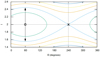 |
Fig. 1 Level curves of a fictitious Hamiltonian. O indicates a stable equilibrium point at (θs = 60°, I0 = 2) and X an unstable equilibrium point at (θu = 240°, I0 = 2). The arrows show the total resonance width, which is 2(Isep − I0), where Isep = 2.44. |
3 Resonance model in Jacobi coordinates
It is also possible to formulate the method in Jacobi coordinates, which are more general than Poincaré coordinates and are particularly well suited for the study of planets evolving in binary stellar systems. Following Lee & Peale (2003), the Hamiltonian in Jacobi coordinates is
 (21)
(21)
where
 (22)
(22)
where ai are the osculating semimajor axes in the Jacobi system, Δi2 are the mutual distances between bodies m2 and mi and r2 are the distance of the mass m2 to the barycenter of the subsystem m0 and m1. The canonical variables are defined in analogy to the Poincaré system, but now we have
 (23)
(23)
 (24)
(24)
We perform the same canonical transformation as in Eq. (4), and then the new Hamiltonian is H(θ, λ2, I1, I2) = H0(I1, I2) − R(θ, λ2, I1, I2), where
 (25)
(25)
We perform a mean on λ2 and obtain aHamiltonian H(θ, I1, I2) analogous to Eq. (6). We can calculate level curves for this Hamiltonian, and the equilibrium points are determined as well as the separatrix.
The equilibrium points verify the same conditions given by Eq. (7). The first condition gives the location of the exact resonance k1 n1 = k2n2, where the mean motions are now  and
and  . The second condition gives the values of thelibration centers θ0, and the stable libration periods are given by Eq. (12), where in this case
 (26)
(26)
and Hθθ = −Rθθ, which is calculated numerically. HII and Hθθ are evaluated at the stable equilibrium point. Following an analogous reasoning as the previous section, we obtain
 (27)
(27)
 (28)
(28)
We show an example in Fig. 2. The expressions above give us the half-widths of the resonances for the general case. For the particular case m2 ∕m1 ~ 0, which corresponds to a planet around a binary system, we obtain  , Δa1 ~ 0 and
 (29)
(29)
This recovers the resonance width for the restricted case (Gallardo 2020) in Jacobi coordinates because in the restricted case, m2 is not present in R. When a planet orbits close to a stellar binary system, the widths estimated by this method may exceed the planet semimajor axis. In this case a better result can be obtained by numerically calculating the borders of the resonance identifying the separatrix using the expression of the Hamiltonian given by Eq. (6). No method can compute the resonance widths for the cases in which the planet is located so close to the binary that close encounters occur that turn its dynamic chaotic.
To avoid erroneous results generated by unrealistic ΔR due to closeencounters, good practice is to monitor the mutual distance when the integral R(θ) is computed and to discard the calculations that are obtained when close encounters occur. A reasonable tolerance criterion could be around three mutual Hill radii, see, for example, Gallardo (2020) and the discussion in the next section.
We recall that our model assumes fixed pericenters and nodes. As they evolve over time, the resonance widths change over time. For a given set of pericenters and nodes, the widths are maximum, and for others they are minimum. This leads to the idea of resonance fragility (Gallardo 2020), a parameter that measures the variability of the widths.
Results obtained with this model are quite good in comparison with the numerical integration of the full equations of motion. They improve the results obtained with analytical methods based in truncated expansions. For the system HD 45364 that was studied by Batygin & Morbidelli (2013), for example, the dynamics is qualitatively well described by an analytical method, but it cannot reproduce the libration frequency correctly. Instead, our model correctly predicts the libration period and provides a good complement to the analytical theory. We show some applications of our model in the next sections.
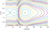 |
Fig. 2 Hamiltonian level curves for a fictitious planetary system composed of a star with m0 = 1 M⊙ and two planets both with mass 0.001 M⊙, mutual inclination of 20°, e1 = 0.5, and e2 = 0.9 located in 3:2 resonance with a1 = 1 au. The stable equilibrium points are shown with an O and the unstable point is shown with an X. We apply Eq. (28) and predict a total width of 0.048 au in a2. |
4 Application to planetary systems
The resonant model described in this paper has several different applications. While it may be employed to study isolated commensurabilities, giving information about the equilibrium solutions, libration periods, and widths, it may also be used to map a region in phase space. It may therefore aid in quantifying the proximity of the system to resonant configurations and identify regions that are susceptible to instabilities stemming from resonance overlap. In certain ways, the model allows us to obtain a qualitative description of the resonant structure of the phase plane for a fraction of the computational cost of a dynamical map (e.g., Megno, Mean Exponential Growth of Nearby Orbits, Cincotta & Simó 2000).
4.1 System HD 31527
In our first application we analyze the orbital evolution and resonant structure in the vicinity of system HD 31527. Discovered by Mayor et al. (2011) and recently revisited by Coffinet et al. (2019), this star hosts three Neptune-size planets orbiting a G0V star with mass m0 = 0.96 M⊙. Even though not all the planetary parameters are provided, it is possible to obtain a best fit of the radial velocity data based on the Data & Analysis Center for Exoplanets1 (DACE; see Buchschacher et al. 2015). Keplerian model initial conditions were computed using the formalism described in Delisle et al. (2016). We quadratically added a noise level of 0.75 m/s to the published radial velocity (RV) uncertainties to take stellar jitter and the typical instrumental noise floor seen in HARPS data into account. In addition to the signals fitted, we allowed an RV offset. Night binning reduces from 256 to 244 the RV data, although the orbital fit remained virtually unchanged.
The results are shown in Table 1, where the error bars in the semimajor axes and masses were estimated from the joint posterior distribution of the model parameters using a Markov chain Monte Carlo (MCMC) analysis (Díaz et al. 2014). Compared with previous estimates, the greatest change in the orbital fit lies in the eccentricity of the outer planet. Mayor et al. (2011) found ed ≃ 0.38, while Coffinet et al. (2019) reported ed ≃ 0.67. Because neither of these works presented estimates for mean longitudes or longitudes of pericenter, no stability check was carried out. To the best of our knowledge, no dynamical studies have been performed, and the long-term orbital evolution of the planet has yet to be determined. Following usual conventions, for our dynamical analysis we denote the inner planet (HD 31527 b) m1, the middle body (HD 31527 c) m2, and the outermost planet (HD 31527 d) m3.
The top graph of Fig. 3 shows the resonant structure in the (a2, e2) plane around the nominal position of the middle planet. The libration width of each commensurability was determined from Eqs. (27)–(28) assuming constant semimajor axes, eccentricities, and longitudes of pericenter. Mutual inclinations were taken equal to zero, and all orbital elements (with the exception of a2 and e2) were assumed equal to their nominal values. Because the resonance widths are determined by the maximum range attained by the orbit-averaged disturbing function (i.e.,  ), the librationwidth increases for initial conditions closer to the collision curves, highlighted in gray. For eccentricities beyond this curve, the maximum value of R can attain very high values that may not be correctly estimated using finite differences. This leads to a resonant structure that appears jagged, irregular, and unreliable. Moreover, very high values of R are associated with close encounters between the planets and with instabilities. In the absence of a suitable protective mechanism (i.e., mean-motion resonance), all trajectories with e2 above the collision curves would lead to a disruption of the system.
It is important to mention that throughout this work, the collision curve was determined numerically from the calculation of the unaveraged disturbing function. For each value of the semimajor axis, we searched for the minimum eccentricity for which the mutual distance between the bodies was zero for some combination of the two mean longitudes. Only within the libration region of an MMR, the correlation between the mean longitudes might allow the planets to avoid the collision point, similarly to Neptune and Pluto, that are able to evade close encounters because their configuration is resonant.
Mean-motion resonances with the inner planet are plotted in red. Their width decreases toward the right-hand side of the plot. Conversely, mean-motion commensurabilities with the outer planet are shown in blue. Significantly thinner because of their higher order, these MMR become less relevant for lower values of the semimajor axis a2.
Because the planetary masses are relatively low, most resonances are thin and the phase space below the collision curve appears dominated by secular interactions. Even the 3/1 MMR between m1 and m2 is barely visible for eccentricities of the order of e2, and its effects are therefore not expected to be significant. Curiously, the nominal location of m2 almost coincides with the 16/3 mean-motion commensurability with the outer planet. Again, however, the width of the MMR in the plot is very small, and there does not appear to be a strong indication of any significant effect on the dynamics of the system.
The bottom graph of Fig. 3 shows a similar resonant map, but now for the semimajor axis and eccentricity plane of the outer body. Only MMRs with m2 are plotted. Even though all commensurabilities are of a high order, the high eccentricity of the planet increases their reach, generating a significant widening of the libration region for values of e3 close to the nominal value. The best-fit solution lies close to the collision curve, and the top of the error bar almost reaches this limit. As in the previous frame, the nominal semimajor axis almost coincides with that of the 16/3 MMR, whose width in this plane is substantially larger than previously seen in (a2, e2). Some effect on the dynamical evolution of the system might be possible after all.
Figure 4 shows a Megno (Cincotta & Simó 2000) dynamical map, again in the (a3, e3) plane, but now focusing on a smaller region around the outer planet. A total of 300 × 300 initial conditions were integrated for 104 yr. All otherorbital elements, including the initial mean anomalies, were set to those given in Table 1. Initial conditions leading to escapes or collisions during the simulation are shown in red. Regular motion (at least within the integration span) is shown with dark colors, and increasingly chaotic trajectories are identified with lighter tones. Only the central region of the stronger MMRs proves to be a protective mechanism that is sufficiently effective to avoid disruptive perturbations and close encounters. These safe zones appear as green stalagmites above the collision curve, shown in gray.
The separatrices of several mean-motion resonances are shown with white lines, the most important of which are identified with rounded labels. To estimate the libration widths, we employed two different approximations. The dashed lines show results obtained without specifying any upper bounds in Rmax. They yield results that are analogous to those in Fig. 3. As before, the resonance widths increase monotonically for higher eccentricities, leading to an overlap of adjacent MMRs for initial conditions close to the collision curve. Because the structures beyond this point may not be reliable, they are not plotted.
In a second calculation, the libration widths were calculated limiting the value of Rmax to configurations where the distance between the planets was larger than a lower bound Δmin. With this approach we aimed to reduce the reach of the commensurability to include only those initial conditions that avoid close encounters and are therefore indicative of stable motion.
Without detailed stability criteria, the necessary value of Δmin can only be estimated qualitatively. For the restricted three-body problem, Gallardo (2020) showed that good agreement with N-body simulations was found using Δmin ~ 3RHill, where RHill is the Hill radius of the perturber. Following the same idea, in the planetary case involving bodies mi and mj, we adopted  , where
![Mathematical equation: \begin{equation*} R_{\textrm{Hill}}^{(i,j)} = \frac{a_i + a_j}{2} \biggl[ \frac{m_i+m_j}{3m_0} \biggr]^{1/3} \end{equation*}](/articles/aa/full_html/2021/02/aa39764-20/aa39764-20-eq38.png) (30)
(30)
is the so-called mutual Hill radius of the planets (Marzari & Weidenschilling 2002). This expression for Δmin is equal to the minimum distance between planets in circular orbits leading to Hill stability, as deduced originally by Marchal & Saari (1975) and Marchal & Bozis (1982), and later made commonly known by Gladman (1993). Although this choice for Δmin does not constitute a credible stability limit for multiplanet systems in eccentric orbits, we found it a simple expression leading to reasonable agreement with N-body simulations. A more rigorous analysis is left for future studies.
The libration widths incorporating Δmin as a minimum distance between the planets are shown with continuous white lines in Fig. 4. The effect of the cutoff starts being noticeable well below the collision curve and reduces the effective size of the stable resonance domain. For the 5/1, 16/3, and 11/2 MMRs the analytical results agree very well with the dynamical map, even though the predicted regions are overestimated. The modified model also predicts finite libration widths for higher-order and weaker commensurabilities; but no corresponding structure is observed in the N-body map.
The nominal position of the outer planet is shown with a large filled yellow circle. The error bars are very evident in both the semimajor axis and the eccentricity. The best fit coincides almost exactly with the 16/3 MMR, but nonresonant trajectories also lie within the error bars. However, most of these solutions are associated with highly chaotic motion, and only the 16/3 MMR appears to be regular. The white lines show that the regions leading to chaotic motion are defined by high-order commensurabilities. The correlation in the libration widths between the dynamical map and the semianalytical model is very good and proves a very useful tool for mapping the overall dynamical characteristics of the system.
To study the resonant motion and long-term stability of the system, we performed an N-body simulation of the nominal solution for ~3 × 10⁶ yr. The calculation of the maximum Lyapunov exponent (LCE) is shown in the lower right-hand frame of Fig. 5, yielding a characteristic time of about τLCE ~ 104 yr. This indicates that the best-fit system is only weakly chaotic, and the departure from a purely regular trajectory should only be noticeable for timescales longer than τLCE, in agreement with the estimated value of ⟨Y ⟩ shown in the previous figure.
The time evolution of the semimajor axis and eccentricity of the outer planet are shown in the top row of Fig. 5. In order to aid the visualization of the resonant and secular periods, only the first 105 yr of the integration are plotted. The solution appears to be completely quasi-periodic, and we found no trace of a secular trend or long-term increase in the amplitudes. Finally, the bottom left-hand graph shows the behavior of the secular angle Δϖ(3,2) = ϖ3 − ϖ2 in green, and the red curve corresponds to the resonant angle
 (31)
(31)
From these results, it appears that the middle and outer planets of the HD 31527 system lie inside the 16/3 MMR, displaying a moderate-amplitude libration around σ2 = π. To the best of our knowledge, this is the first time that an exoplanetary system is found in such a high-order and high-degree mean-motion commensurability, and whose resonant motion acts as an effective protection mechanism. The chaoticity of the surrounding regions is so strong that it is difficult to imagine a formation scenario for this system involving planetary migration, even if this process were responsible for the excitation of the eccentricity. Two stronger MMRs (5/1 and 11/2) are found close by and to either side of the present-day position; it is hard to imagine how these could have been avoided while capturing the system in the (weaker) 16/3 resonance.
The difference in longitude of pericenter between these planets oscillates around Δϖ(3,2) = π with a secular period of about Tsec ≃ 5000 yr. When the eccentricity of the middle planet approaches zero, the secular angle spikes and circles rapidly. This behavior is not related to any chaotic motion, however.
The libration period may also be estimated with the semianalytical model and yields a value of Tlib ≃ 22 yr, while a Fourier decomposition of the N-body simulation yields a value close to ~19 yr. We believe the agreement is very satisfactory, particularly considering that the analytical estimate corresponds to zero-amplitude librations, while the numerical solution has a considerable oscillation around the fixed point. This calculation additionally shows that the model may be used to obtain qualitative information on the resonant dynamics, regardless of the eccentricity or mutual inclination of the bodies.
Minimum masses and orbits for system HD 31527.
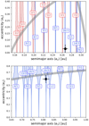 |
Fig. 3 Resonant structure determined with the semianalytical model in the (a2, e2) plane surrounding the middle planet (top) and in the (a3, e3) plane (bottom). Two-planet commensurabilities between planets m1 and m2 are shown in red, and those between the middle and outer planets are presented in blue. In both plots the nominal positions of the planets are identified by filled black circles, and the collision curves are depicted in gray. |
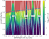 |
Fig. 4 Megno map for the HD 31527 system, as obtained from the numerical integration of a grid of 300 × 300 initial conditions in the (a3, e3) plane. All other orbital elements were set to the nominal values. Integration time was set to 104 yr, and escapes during this time span are highlighted in red. The color code shows values of (⟨Y ⟩ − 2). Dark blue corresponds to more regular orbits, and lighter tones of green indicate increasingly chaotic motion. The location of the outer planet is shown with a filled yellow circle, and the collision curve is plotted in gray. The libration widths of the most relevant MMRs determined analytically are plotted as white lines. See text for details. |
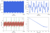 |
Fig. 5 Results of a long-term N-body simulation of the nominal solution for system HD 31527. Top rows: semimajor axis a3 and eccentricity e3 of the outer planet as a function of time for the first 105 yr of the integration. Lower left-hand plot: shows in green the difference in longitude of pericenter ϖ3 − ϖ2, and the red curve presents the behavior of the resonant angle σ2 = 3λ2 − 16λ3 + 13ϖ3. Lower right-hand graph: maximum Lyapunov exponent for the system during the complete simulation. |
4.2 System HD 74156
In the early 2000s it was suggested that most planetary systems should be dynamically packed (e.g., Barnes & Quinn 2001; Barnes & Raymond 2004), with little room for additional bodies between adjacent planets (e.g., Giuppone et al. 2013). Based on this idea, several works analyzed the phase space of known systems searching for stable regions that may host undetected planets. One of these systems was HD 74156.
Discovered by Naef et al. (2004), the system hosts two currently confirmed planets that orbit a m0 = 1.24 M⊙ star. One of the bodies lies close to the star with an orbital period of Pb ≃ 60 days, and the second body is found significantly farther out (Pc ≃ 5.5 yr). After a series of N-body simulations, Raymond & Barnes (2005) found that a Saturn-type planet could well exist between the two known bodies and that the resulting system would be stable for timescales on the order of the age of the star.
As new observations became available, Barnes et al. (2008) extended the numerical study and further constrained the mass and orbit of the hypothetical third planet to the new radial velocity data. They found that the region between the two confirmed planets contains a rich dynamical structure defined by both isolated and interacting mean-motion resonances with the two bodies. The most promising system configuration is reproduced in Table 2.
Unfortunately, subsequent orbital fits including stellar jitter (Baluev 2009) did not confirm planet d, arguing that its signal could be due to annual systematic errors from the High Resolution Spectrograph (HRS) of the Hobby-Eberly Telescope. Wittenmyer et al. (2009), Meschiari et al. (2011), and Feng et al. (2015) later updated the system with additional observations and also failed to detect the proposed middle planet.
However, the resulting dynamical structure of the three-planet system proposed by Barnes et al. (2008) proved sufficiently interesting to be a good test for our model. Even if the third planet may not exist, the hypothetical extended system constitutes a challenging benchmark for the predictive power of the model, as well as for its capacity of identifying underlying features in the dynamical maps.
As before, we numbered the planets according to their distance to the central star, as identifiedin the lower row in Table 2. The confirmed planets are thus m1 and m3, and the proposed unconfirmedbody is labeled m2. Because we study a hypothetical system, we need not be tied to specific values for the angles. We therefore modified the orbital elements given in Table 2 such that
 (32)
(32)
In other words, all planets are assumed to lie on their pericenters, and the difference in the initial apsidal orientation between adjacent bodies is taken to be Δϖ(2,1) = ϖ2 − ϖ1 = 0 and Δϖ(3,2) = ϖ3 − ϖ2 = π. This choice helps preserve the symmetry in the libration regions in the dynamical map and in some cases maximizes their width.
For the representative plane, we chose the (a2, e2) plane, more or less centered on the proposed position of the middle planet, and with limits similar to those used in Fig. 2 of Barnes et al. (2008). The left-hand plots of Fig. 6 show color plots of Δe for a grid of 900 × 900 initial conditions varying the values of the semimajor axis a2 and eccentricity e2 while maintaining all other orbital elements fixed. Each initial condition was then integrated for 103 yr, keeping track of any ejections or collisions during this time. The color code corresponds to the maximum change in eccentricity of m2 during the integration (i.e., Δe = max(e2) −min(e2)), and has proven to be a powerful indicator of secular and resonant dynamics (e.g., Dvorak et al. 2004; Ramos et al. 2015).
While the vertical light-toned plumes are generated by the action of mean-motion resonances, the dark diagonal stripe in the upper left-hand plot represents the so-called Mode I secular mode (Michtchenko & Malhotra 2004) between the inner and middle planet and represents the locus of initial conditions leading to zero-amplitude oscillation of the secular angle Δϖ(2,1) around zero. In the plot the Mode I secular mode may be seen as a diagonal curve running from (a2, e2) ≃ (0.8, 0.2) down to (a2, e2) ≃ (0.95, 0.1). An analogous but less evident stripe may also be seen in the lower left-hand plot for higher values of the semimajor axis. Because the longitude of pericenter of the outer planet was chosen such that Δϖ(3,2) = π, no indication of a Mode I with the outer planet is observed.
For the right-hand plots, we reduced the grid to a set of 300 × 300 initial conditions, but extended the integration time to 104 yr. The color code now shows the Megno values at the end of the simulation. As in the dynamical map constructed for the previous planetary system, dark blue corresponds to regular orbits, while lighter tones represent increasingly chaotic trajectories. In both sets of graphs, the semimajor axis domain was split into two sections: the region with a2 ≤ 0.95 au is shown in the top frames, and the bottom graphs show results for a2 ≥ 0.95 au. The position of the proposed planet is highlighted with filled white circles.
The maximum widths of the relevant MMRs as obtained with the model are shown with red lines (for commensurabilities with the inner planet) and blue lines (for resonances with the outer planet). They are identified in the top partof the graphs using text with the corresponding color. In most cases we note very good agreement between thepredicted resonant structure and the dynamical maps. For example, the hour-glass figure centered at a2 ≃ 0.86 au is caused by the 5/1 MMR with the inner planet. For eccentricities e2 ≲ 0.13, the stable equilibrium solution occurs for σ = λ1 − 5λ2 + 4ϖ2 = π, resulting in chaotic trajectories inside the separatrix. Conversely, for higher eccentricities, the stable solution occurs for values of the resonant angle σ = 0 and is thus coincidental with the angles used to define the representative plane. The central region of the resonance is therefore more regular and admits librational solutions.
These hour-glass structures observed for the 5/1 MMR are not new and were detected in studies of circumbinary planets by Zoppetti et al. (2018). The center of the X shape appears to coincide with the forced eccentricity of the planet (Zoppetti et al. 2019), a correlation that also appears in the plots shown here.
Another interesting feature is the large chaotic region located at a2 ≃ 0.96 au and visible in the lower plot. The resonance analysis shows that it is generated by the interaction between two distinct commensurabilities, the 6/1 between planets m1 and m2, and the 8/1 resonance between m2 and m3. A similar structure occurs at a2 ≃ 1.06 au between two 7/1 MMRs, but the overlap does not occur for near-circular orbits this time, which leads to a wedge-shaped region of regular motion at low eccentricities.
For a more general analysis of the phase plane, we recall that an ni ∕nj = k2∕k1 MMR has two independent resonant angles that we may denote by
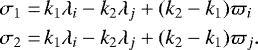 (33)
(33)
All other possible critical angles may be written as linear combinations of σ1, σ2 and the difference in longitudes of pericenter. Our model analyzes the behavior of the resonances based on the study of the combination k1 λi − k2λj, independent of the definition of σ. We can calculate the location of the equilibrium points corresponding to σ1, for example, and we can analyze how the predictions of this model correlate with the dynamical structures found in the Megno map. Nevertheless, the model can also be used to separate the mean-motion resonances into three distinct groups, according to the number of stable solutions of σ = σ1 and their equilibrium values. These are detailed below.
The first group corresponds to two-planet commensurabilities, between the middle planet m2 and one of its neighbors, in which a the stable equilibrium solution corresponds to a value of the resonant angle σ = 0. Examples are dc-10/1, bd-11/2, dc-17/2, bd-6/1, dc-15/2, and bd-13/2. Following the notation used in the figure, the letters indicate the planets involved in the MMR. These solutions are found to be stable for all the values of e2 up to the edge of the collision curve. In some cases, these solutions are stable only for a certain range of eccentricities. These include bd-5/1 (for e2 ≳ 0.13), dc-8/1 (e2 ≳ 0.01), and bd-7/1 (e2 ≳ 0.1).
The second group is similar to the previous case, but these resonances are characterized by a single stable solution located at σ = π. An example is dc-9/1. Most of these solutions are found for a limited interval of the eccentricity e2, however. These include bd-5/1 (for e2 ≲ 0.13), bd-7/1 (e2 ≲ 0.1), and dc-7/1 (e2 ≳ 0.05). In these cases the solutions found for other eccentricities usually correspond to σ = 0 librations.
Finally, the third group corresponds to the case of asymmetric stable solutions that harbors fixed points with values of σ different from 0 or π. Examples were found only in resonances with the outer planet and include dc-7/1 (for e2 ≲ 0.05) and dc-8/1 (for e2 ≲ 0.01). For higher eccentricities, these solutions reduce to symmetric librations, either with σ = 0 or σ = π.
In general, the behavior of resonant initial conditions in the dynamical map agrees very well with the behavior expected from the model. Thus, resonances with stable solutions in σ = k2π are expected to show regular solution inside the libration domain for the chosen representative plane. This behavior is clearly observed in both the dc-10/1 and dc-9/1 commensurabilities and to lesser degree in the bd-5/1 resonance.
Conversely, resonances with stable solutions in σ = π should exhibit more chaotic motion in the representative plane. This prediction is observed in the case of dc-7/1 and, for example, low-eccentricity initial conditions in the bd-5/1 resonance. It is important to recall, however, that there is no unique resonant angle, particularly for high-order MMRs, and the most dominant combination between themean longitudes and longitudes of pericenter depends on the eccentricities and relative masses of the planets involved in the commensurability. Even so, the information that the model yields still serves as an initial analysis of the resonance, and serves to identify characteristics or interesting features that deserve further study.
Masses and orbital parameters of the three-planet HD 74156 system proposed by Barnes et al. (2008).
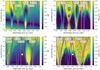 |
Fig. 6 Top and bottom left-hand graphs: Δe dynamicalmap for system HD 74156 as obtained from the numerical integration of a grid of 900 × 900 initial conditions in the (a2, e2) plane. Upperplot: corresponds to a semimajor axis a2 ∈ [0.80, 0.95] au, and the bottom panel to a semimajor axis a2 ∈ [0.95, 1.10] au. The integration time was set to 103 yr, and escapes during this time span are highlighted in light yellow. The location of the middle planet is shown with a filled white circle. The libration widths of the most relevant MMRs determined analytically are highlighted in blue (resonances with the outer planet) and red (resonance with the inner planet). Top and bottomright-hand graphs: Megno map for the same plane. The set of initial conditions was reduced to a 300 × 300 grid, but the integration time was extended to 104 yr. |
5 Application to circumbinary planets
The Kepler mission revolutionized our knowledge of the existence of circumbinary planets (CBPs), with the discovery of 13 transiting CBPs orbiting 11 Kepler eclipsing binaries. Recently, the first circumbinary planet was reported using the data from TESS mission (TOI 1338, Kostov et al. 2020). These planets bring new challenges for formation theories, and their formation mechanism is still debated because most of them lie near their instability boundary at about three to five binary separations. Recent studies have argued that the occurrence rate of giant Kepler-like CBPs is comparable to that of giant planets in single-star systems (see Martin et al. 2019, and references therein).
In this sample, all the transiting binaries that host planets have short periods (< 30 days) (Schwarz et al. 2016) with eccentricities ranging from quasi-circular orbits (like Kepler-47, Orosz et al. 2012b) to highly eccentric (like Kepler-34, Welsh et al. 2012). Typical planets detected around binary stellar systems have a radius of about 10 Earth radii and orbital periods of about 160 days on almost circular coplanar orbits (i.e., ap ~ 0.35 au), Martin (2018).
Transiting inclined CBPs are more difficult to detect because the selection bias. However, planets do form in circumbinary disks (CBDs), and highly noncoplanar CBDs such as 99 Herculis (Kennedy et al. 2012), IRS 43 (Brinch et al. 2016), GG Tau (Cazzoletti et al. 2017; Aly et al. 2018), HD 142527 (Avenhaus et al. 2017), and HD 98800 (Kennedy et al. 2019) were detected.
Previous analysis of the stability of inclined massless particles was reported by Doolin & Blundell (2011), who considered different binary eccentricities and mass ratios between its components. More recently, Cuello & Giuppone (2019) and Giuppone & Cuello (2019) studied the evolution of CBDs and the stability of inclined Jupiter-like planets around binaries. Recently, circumbinary retrograde coplanar stability was addressed by Hong & van Putten (2021) for circular and eccentric planets. Furthermore, there is some evidence that the N∕1 MMRs are related to the planetary parking location and their evolution in the disk. With a simplified model, Zoppetti et al. (2018) suggested capture in 5/1 MMR and subsequent tidal evolution of the planet, whereas some effort with fine-tuning hydrodynamical simulations tried to place some constraints on the protoplanetary disks that allow migration of CB planets, but do not show capture at MMRs (see, e.g., Penzlin et al. 2020, and references therein).
In this section we study the N∕1 and N∕2 mean-motion resonances (identified as k2∕k1 in the model). Our aim is to correlate unstable regions near the binary with the MMR overlap.
We used the model described in Sect. 3 to map a region in phase space, identifying regions susceptible to instabilities stemming from resonance overlap. Regular motion and chaos of a coplanar CBP in the plane (α, e) are presented in Sect. 5.1 (with α = a∕aB), and we study an inclined CBP in the plane (a, i) that is initially placed on a circular orbit in Sect. 5.2. We consider different types of binaries such those detected by Kepler and TESS. We do not expect effects on the binary orbit because the mass of the planet is much lower than that of the binary companion. To describe the orbit of the binary, we use orbital elements with subindex B, and orbital elements without subindex for the planet. Without loss of generality, we set initial conditions {λB = 0°, ϖB = 0°, ΩB = 0°}. Our fiducial binary has aB = 0.1 au, and the sum of the component masses is equal to 1. The angles of a given planet are measured from the direction of the binary pericenter, and Jacobi orbital elements of the circumbinary planet are given without subscripts.
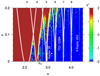 |
Fig. 7 Megno map for a circumbinary system in the (a, e) plane. The color code shows values of Y* = log10(⟨Y ⟩− 2). Dark blue corresponds to more regular orbits, and lighter tones of green indicate increasingly chaotic motion. The libration widths of the most relevant MMRs determined with the model are plotted as white lines, setting ϖ = 180o. The top scale indicates the positions of N∕1 resonances with respect to the mean motion of the binary. See text for details. |
5.1 Coplanar circumbinary planets
In this subsection we start with coplanar orbits, and we only show the location of the MMR in the plane (α, e) for a binary with a mass ratio q = 0.2 and eccentricity eB = 0.1, defining α = a∕aB. Figure 7 shows a Megno dynamical map for a planet, focusing on a region between 1.5 < α < 4.5. A total of 250 × 100 initial conditions were integrated for 104 binary periods. All angular elements were set to zero. Initial conditions leading to escapes or collisions during the simulation are shown in brown.
The semianalytical model predicts that all the N∕1 MMRs have one stable center of resonance around 0°, in the region plotted in Fig. 7. However, maybe because of the fast precession of ϖ induced by the binary (see Farago & Laskar 2010; Li et al. 2014), closer resonances are unstable (3∕1 and 4∕1). In contrast to the planetary case, we identify that regions inside of the stronger N∕1 MMRs are chaotic (mainly observed in MMR 3∕1 and 4∕1). Overlap of 3∕1, 4∕1, and 5∕1 delimits the unstable regions in the plane (α, e), showing a perfect agreement of the model with numerical integrations. The V -shape of each resonance is evident and the resonant-width decreases as we increase N; it is almost zero for circular planets.
Additionally, we plot in Fig. 7 the position of some similar CB systems with the orbital parameters listed in Table 3. We indicate with αc the minimum stable coplanar-prograde semimajor axis, using the criteria of Holman & Wiegert (1999). This empirical criterion, which is widely used, is based in a polynomial fit that considers quadratical exponents of aB, eB, and q. According to Fig. 7, this limit roughly corresponds to the closest region to the binary where secular motion is allowed (at the correct position of MMR 4/1).
We verified that the dynamical maps do not show a difference in the closer regions when we chose initial conditions with Δϖ = 0o or with Δϖ = 180o. We must note that in regions farther away from the binary, differences in structures appear inside the resonance, as shown in Fig. 3 of Zoppetti et al. (2018).
Masses and orbital parameters of CB planets.
5.2 Inclined circumbinary planets
In the view of variety of CBDs around binaries and to test the model for arbitrary inclination, we studied the dynamics of inclined planets around binaries (P-type planets). We must note that for inclined particles, the nodal libration (the regions in which inclination and node librates) is determined by the separatrix F, simplifying the expression of Farago & Laskar (2010),
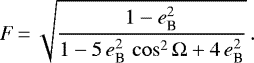 (34)
(34)
Then, libration of the node Ω and inclination i of the CB planet around 90o is expected when
 (35)
(35)
It is important also to remark that outside the separatrix region, Ω circulates (prograde or retrograde direction). We recall that librating orbits and stationary angles change when brown dwarf companions are considered (Chen et al. 2019), that is, for masses that are not compatible with CB detected planets.
We explored the MMR location and widths around a wide variety of circumbinary inclined orbits for different binary mass ratios q = {0.2, 0.5, 1}. However, we chose to center our attention on three particular configurations for a mass ratio q = 0.2. We used Eq. (28) of the semianalytical model to calculate the width of the resonances, although we can numerically search for the exact extension of each separatrix to estimate their interior and exterior limit. We found that 2∕1 MMR alone exhibits appreciable differences between Eq. (28) and the exact extension deduced from the level curves of the Hamiltonian. Although our planet was initially placed on circular orbits, the mean value of the planet eccentricity in regular orbits is roughly e ~ 0.05 due to the excitation induced by the binary, and we used this value to calculate the width of the resonances.
The dynamics of CB inclined planets at these distances leads to circulation of ϖ because of the interaction with the binary. Moreover, outside the nodal resonances, the node Ω circulates (Farago & Laskar 2010; Doolin & Blundell 2011; Li et al. 2014). Our model calculates the width of the resonance for a fixed value of ϖ and Ω, and we analyzed the dependence of widths for different values from 0° to 180°. We show the results in Fig. 8, setting a binary with q = 0.2 and aB = 0.1 au. At first sight, we observe common features in all the panels, where the width of resonances decreases with increasing N and the prograde resonances are wider than retrograde resonances. The changes in the width of the separatrices due to different values of ϖ (left panels) are higher than when we change initial values of Ω (right panels). Furthermore, for the cases when we set initial Ω = 90° the separatrices show a wobbling shape at high inclinations. Additionally, the effect of change the value of Ω have also profound effects in separatrices of retrograde orbits, blurring the regions around 2/1, 3/1 and 4/1 MMR (see middle frames at Fig. 8).
In each left-hand panel we indicate with ac the minimum stable coplanar-prograde semimajor axis using the criterion of Holman & Wiegert (1999). According to Fig. 8, this limit roughly correspond to the closest region to the binary where secular motion is allowed (outside the resonance overlap region).
The difference between the top and middle frames of Fig. 8 is the eccentricity of the binary. For a low eccentricity of the binary (eB = 0.1 at top frames), we observe the region of superposition in coplanar prograde orbits between 2/1 and 3/1 MMR when we set different ϖ values, while the other resonances almost remain constant. The change in Ω in the top right frame does not affect the coplanar prograde or retrograde resonances. When we increase the eccentricity of the binary (eB = 0.5, center frames), the separatrix at prograde coplanar resonances shows huge changes: they overlap up to the 6/1 MMR. Retrograde resonances are less affected, and the location of the 4/1 MMR is associated with the most stable region near the binary. Islands of stable motion are possible, where the gray lines do not cross at polar inclinations i ~ 90°.
Varying Ω (center right-frame) does not affect the width of the low-inclined prograde resonances, but enhances the width of the highly inclined retrograde resonances. In the bottom left frame of Fig. 8 we plot the resonance widths for a fixed value of Ω = 0° and varying ϖ, where the initial conditions are outside the libration region of Ω. The separatrix location encompasses wider regions in coplanar and highly inclined systems, while for retrograde coplanar orbits, the separatrices shrink and leave favorable conditions for regular orbits closer to the binary. The bottom right frame shows a separatrix extension for ϖ = 90° and different fixed values of Ω, where inclined orbits are more affected by this variation.
Some works showed dynamical maps around binaries in the plane (a, i) using ejection times (see, e.g., Doolin & Blundell 2011) or the Megno indicator (see, e.g., Cuello & Giuppone 2019; Giuppone & Cuello 2019) but did not convincingly explain the regular spatial motion. To compare with the model, we ran numerical integrations and show the results in Fig. 9 using the color scale Y* = log10(⟨Y ⟩− 2), where ⟨Y ⟩ is the Megno indicator. We also overplot the N∕1 resonances that we constructed for the Fig. 8. The planet has initial ϖ = 0°, e = 0, and the binary mass ratio is q = 0.2. Each frame is constructed from the numerical integration of a grid of 300 × 300 initial conditions in the (a, i) plane. All other initial orbital elements were set to the nominal values. Integration time was set to 3 × 10² yr (~ 104 orbital periods of the binary).
The top frame of Fig. 9 shows eB = 0.1 (almost like Kepler-38, Kepler-453, or TOI-1338), where unstable regions coincide with the overlap of the N∕1 resonances. While the prograde MMRs have considerable widths, the MMR widths shrink with increasing inclination. The reported stability island around polar orbits (see, e.g., Doolin & Blundell 2011; Cuello & Giuppone 2019; Giuppone & Cuello 2019) are easily explained with the resonance width of the MMR at highly inclined orbits (i around 90o). Moreover, as the inclination increases, the resonance width decreased; retrograde resonances are more compact.
When we increase the binary eccentricity eB = 0.5 (center and bottom frames of Fig. 9, similar to Kepler-34), more chaotic regions near the binary at coplanar prograde and retrograde orbits appear as result of resonance overlap (see the center frames of Fig. 8). Regular orbits closer to the binary survive at i ~ 90°. Finally, in the bottom frame of Fig. 9 we show the case were eB = 0.5 but dynamical maps with initial Ω = 0° (i.e., Ω does not fall inside the nodal libration region for any inclination and always circulates). Unstable regions of low-inclination prograde orbits appear that agree with the N/1 plotted resonances. We recall that the circulation of ϖ causes the overlap that is observed in the bottom frame of Fig. 8.
A shift in semimajor axis for the location of the nominal MMR is evident in the dynamical maps. This shift is higher when the mass ratio q or the binary eccentricity eB are increased (only by about 1% in the case of a binary with q = 0.2 and eB = 0.1). This shift is also present for mean values of the semimajor axis for the dynamical maps.
Finally, in Fig. 10 we compare the width of MMR N∕1 and N∕2 around a binary with eccentricity eB = 0.5 in the plane (a, i) for different mass ratios q = 0.2 and q = 1. We set fixed values of Ω = 90° and ϖ = 0°. The mass ratio of the binary components considerably modifies the width of the MMRs in prograde orbits (see, e.g., 2∕1, 5∕2, 3∕1, and 4∕1). In prograde orbits, the 2∕1 resonance ismost important for determining instability regions because it overlaps regions of the 4∕1 resonance (or the 5/1 resonance, depending on the mass ratio).
Retrograde highly inclined resonances hardly change their width with the mass ratio. For initial values of Ω = 90°, the wobbling structure of the resonances changes with q and i; although is easy to identify regular motion islands beyond the position of the 3∕1 resonance. The N∕2 resonances are thinner thanthe N∕1 resonance; but because of their location between two consecutive N/1 resonances, they overlap in regions that cause the chaos in retrograde configurations (see the top axis in Fig. 8). This shows that the model is useful for interpreting inclined unstable regions around binaries. We verified its validity for a wide combination of orbital parameters.
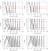 |
Fig. 8 Widths and location of N/1 resonances setting different values of ϖ (left frames) and Ω (right frames) for a planet around a binary with a mass ratio q = 0.2 and aB = 0.1 in the plane (a, i). The top scale of each frame indicates the positions of N∕1 resonances with respect to the mean motion of the binary. We calculate each resonance with the semianalytical model for 20 different values of ϖ in the left-hand frames (Ω in the right-hand frames) from 0° to 180° and plot each one with gray lines. Black lines denote the value for ϖ = 180° (left frames) or Ω = 180° (right frames). Horizontal red lines indicate the separatrix location for nodal libration, i.e., regions in which the dynamics only allow libration of Ω around 90°. See text formore detail. Bottom panels: do not present horizontal lines because the nodal resonance is absent, then Ω circulates independently of the inclination i. |
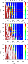 |
Fig. 9 Megno maps of inclined Jupiter planets around a binary with (eB, Ω) = (0.1, 90°), (eB, Ω) = (0.5, 90°), and (eB, Ω) = (0.5, 0°) from top to bottom panels respectively. As before, top scale of each frame indicates the positions of N∕1 MMR and horizontal red lines delimit the nodal separatrix using Eq. (35). White lines are the separatrices of each N∕1 resonances using the semianalytical model, varying the values of Ω and ϖ (equivalent to gray lines in Fig. 8). See text for details. |
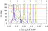 |
Fig. 10 Resonance N∕1 and N∕2 widths setting a different mass ratio between components q = {0.2, 1} in the plane (a, i) calculated with the semianalytical model. For q = 0.2 we use green (N∕1) and magenta(N∕2), and for q = 1 we use orange (N∕1) and blue (N∕2) resonances. Horizontal lines indicate the separatrix location for nodal libration. See text for more detail. |
6 Conclusions
We presented a semianalytical model for planetary mean-motion resonances around a single star or binary stars, yielding the location andstability of fixed points of the averaged system, the libration period of small-amplitude oscillations, and the widths of the librationregion in the semimajor axis domain. It is a natural extension of the model developed by Gallardo (2020) for the restricted three-body problem.
Applications to the HD 31527 and HD 74156 planetary systems, as well as to fictitious and real circumbinary planets show very good agreement between the model predictions and dynamical features deduced from pure N-body simulations, even for very high eccentricities. These dynamical characteristics include the resonance widths, the libration periods, and the stability of the fixed points. Together, these features allow a more detailed interpretation of the dynamical maps and help estimate regions corresponding to long-term orbital stability.
The new orbital fit of the radial velocity data of HD 31527 we presented shows that the middle and outer planets are probably locked in a 16/3 mean-motion resonance and a high-eccentricity moderate-amplitude libration of the resonant angle 16λ3 − 3λ2 − 13ϖ2. This configuration appears to be stable for timescales of at least about 107 yr. Because no significant secular changes in the semimajor axes or eccentricities are observed within this time frame, it is possible that the orbital fit is even stable for timescales comparable to the age of the star.
Differences between predicted and observed widths, as well as the location of the resonance centers, can be attributed to long-term variations in the secular angles (i.e., longitudes of pericenter and ascending nodes) that are assumed constant in the model. These effects are almost negligible in MMR among planetary bodies, but they become more visible in binary systems, especially for high mass-ratios between the stellar components. Notwithstanding this effect, the general features of the resonant dynamics are well reproduced by the model.
Using the semianalytical model, we convincingly demonstrated that for P-type orbits (circumbinary planets), the N/1 MMR overlap is directly associated with the instability limit in the regions closer to the binary. We compared our results with dynamical maps in planes (α, e) and (a, i).
When we analyzed the MMR experienced by an inclined planet around a binary, we found that prograde resonances are wider than retrograde resonances, and the N/1 resonance overlap is the main cause of instabilities near the binary. The N/2 resonances are considerably weaker than the N/1 resonance, but the former contribute to the overlap between consecutive N/1 resonances. We found that N∕1 and N∕2 resonances delimit the islands of stability for polar configurations and that the resonance shape in the plane (a, i) strongly depends on the initial value of Ω, either 0° or 90° for polar inclinations. As we approach the binary, the proximity causes circulation of Ω and ϖ is on short timescales, thus the separatrix of each resonance moves and creates a wider effective separatrix.
The model assumes that the center of the libration domain coincides with the nominal position of the resonance. Although this approximation has been proved to be very reliable in most cases, some values of the system parameters lead to a noticeable offset that appears as a shift of the resonant structure in the semimajor axis domain. While this issue is rarely observable in planetary systems around single stars, it becomes more evident for circumbinary planets with high values of the mass ratio q or binary eccentricity eB. A more detailed study of the resonance offset, as well as its description, is left for a forthcoming work.
Codes for the computation of the resonances can be found online2.
Acknowledgements
We thank the anonymous reviewer who, through a rigorous examination of the manuscript, suggested substantial improvements to this final version. N-body computations were performed at Mulatona Cluster from CCAD-UNC, which is part of SNCAD-MinCyT, Argentina. T.G. acknowledges support from PEDECIBA. C.G. acknowledges the training acquired in the 2020 Sagan Exoplanet Summer Virtual Workshop.
References
- Aly, H., Lodato, G., & Cazzoletti, P. 2018, MNRAS, 480, 4738 [NASA ADS] [Google Scholar]
- Antoniadou, K. I., & Voyatzis, G. 2013, Celest. Mech. Dyn. Astron., 115, 161 [Google Scholar]
- Avenhaus, H., Quanz, S. P., Schmid, H. M., et al. 2017, AJ, 154, 33 [Google Scholar]
- Baluev, R. V. 2009, MNRAS, 393, 969 [NASA ADS] [CrossRef] [Google Scholar]
- Barnes, R., & Quinn, T. 2001, ApJ, 550, 884 [Google Scholar]
- Barnes, R., & Raymond, S. N. 2004, ApJ, 617, 569 [Google Scholar]
- Barnes, R., Goździewski, K., & Raymond, S. N. 2008, ApJ, 680, L57 [Google Scholar]
- Batygin, K., & Morbidelli, A. 2013, A&A, 556, A28 [NASA ADS] [CrossRef] [EDP Sciences] [Google Scholar]
- Beaugé, C., & Michtchenko, T. A. 2003, MNRAS, 341, 760 [Google Scholar]
- Brinch, C., Jørgensen, J. K., Hogerheijde, M. R., Nelson, R. P., & Gressel, O. 2016, ApJ, 830, L16 [Google Scholar]
- Buchschacher, N., Ségransan, D., Udry, S., & Díaz, R. 2015, ASP Conf. Ser., 495, 7 [Google Scholar]
- Cazzoletti, P., Ricci, L., Birnstiel, T., & Lodato, G. 2017, A&A, 599, A102 [NASA ADS] [CrossRef] [EDP Sciences] [Google Scholar]
- Chen, C., Franchini, A., Lubow, S. H., & Martin, R. G. 2019, MNRAS, 490, 5634 [Google Scholar]
- Cincotta, P. M., & Simó, C. 2000, A&AS, 147, 205 [NASA ADS] [CrossRef] [EDP Sciences] [Google Scholar]
- Coffinet, A., Lovis, C., Dumusque, X., & Pepe, F. 2019, A&A, 629, A27 [NASA ADS] [CrossRef] [EDP Sciences] [Google Scholar]
- Cuello, N., & Giuppone, C. A. 2019, A&A, 628, A119 [CrossRef] [EDP Sciences] [Google Scholar]
- Deck, K. M., Payne, M., & Holman, M. J. 2013, ApJ, 774, 129 [Google Scholar]
- Delisle, J. B. 2017, A&A, 605, A96 [NASA ADS] [CrossRef] [EDP Sciences] [Google Scholar]
- Delisle, J. B., Ségransan, D., Buchschacher, N., & Alesina, F. 2016, A&A, 590, A134 [NASA ADS] [CrossRef] [EDP Sciences] [Google Scholar]
- Díaz, R. F., Almenara, J. M., Santerne, A., et al. 2014, MNRAS, 441, 983 [Google Scholar]
- Doolin, S., & Blundell, K. M. 2011, MNRAS, 418, 2656 [Google Scholar]
- Dvorak, R., Pilat-Lohinger, E., Schwarz, R., & Freistetter, F. 2004, A&A, 426, L37 [NASA ADS] [CrossRef] [EDP Sciences] [Google Scholar]
- Farago, F., & Laskar, J. 2010, MNRAS, 401, 1189 [Google Scholar]
- Feng, Y. K., Wright, J. T., Nelson, B., et al. 2015, ApJ, 800, 22 [Google Scholar]
- Ferraz-Mello, S., Mitchtchenko, T. A., & Beaugé, C. 2006, Chaotic Worlds: from Order to Disorder in Gravitational N-body Dynamical Systems, eds. B. A. Steves, A. J. Maciejewski, & M. Hendry (Dordrecht: Springer), 255 [Google Scholar]
- Gallardo, T. 2006, Icarus, 184, 29 [Google Scholar]
- Gallardo, T. 2020, Celest. Mech. Dyn. Astron., 132, 9 [Google Scholar]
- Gallardo, T., Coito, L., & Badano, L. 2016, Icarus, 274, 83 [Google Scholar]
- Giuppone, C. A., & Cuello, N. 2019, J. Phys. Conf. Ser., 1365, 012023 [Google Scholar]
- Giuppone, C. A., Morais, M. H. M., & Correia, A. C. M. 2013, MNRAS, 436, 3547 [Google Scholar]
- Gladman, B. 1993, Icarus, 106, 247 [Google Scholar]
- Holman, M. J., & Wiegert, P. A. 1999, AJ, 117, 621 [Google Scholar]
- Hong, C., & van Putten, M. H. P. M. 2021, New Astron., 84, 101516 [Google Scholar]
- Kennedy, G. M., Wyatt, M. C., Sibthorpe, B., et al. 2012, MNRAS, 421, 2264 [Google Scholar]
- Kennedy, G. M., Matrà, L., Facchini, S., et al. 2019, Nat. Astron., 189 [Google Scholar]
- Kostov, V. B., Orosz, J. A., Feinstein, A. D., et al. 2020, AJ, 159, 253 [Google Scholar]
- Laskar, J. 1991, Series B, NATO Advanced Science Institutes (ASI), 271, 93 [Google Scholar]
- Laskar, J., & Robutel, P. 1995, Celest. Mech. Dyn. Astron., 62, 193 [Google Scholar]
- Lee, M. H., & Peale, S. J. 2003, ApJ, 592, 1201 [Google Scholar]
- Li, D., Zhou, J.-L., & Zhang, H. 2014, MNRAS, 437, 3832 [Google Scholar]
- Marchal, C., & Bozis, G. 1982, Celest. Mech., 26, 311 [Google Scholar]
- Marchal, C., & Saari, D. G. 1975, Celest. Mech., 12, 115 [Google Scholar]
- Martin, D. V. 2018, Populations of Planets in Multiple Star Systems (Berlin: Springer), 156 [Google Scholar]
- Martin, D. V., Triaud, A. H. M. J., Udry, S., et al. 2019, A&A 624, A68 [NASA ADS] [CrossRef] [EDP Sciences] [Google Scholar]
- Marzari, F., & Weidenschilling, S. J. 2002, Icarus, 156, 570 [Google Scholar]
- Mayor, M., Marmier, M., Lovis, C., et al. 2011, ArXiv e-prints [arXiv:1109.2497] [Google Scholar]
- Meschiari, S., Laughlin, G., Vogt, S. S., et al. 2011, ApJ, 727, 117 [Google Scholar]
- Michtchenko, T. A., & Malhotra, R. 2004, Icarus, 168, 237 [Google Scholar]
- Morais, M. H. M., & Giuppone, C. A. 2012, MNRAS, 424, 52 [Google Scholar]
- Naef, D., Mayor, M., Beuzit, J. L., et al. 2004, A&A, 414, 351 [NASA ADS] [CrossRef] [EDP Sciences] [Google Scholar]
- Orosz, J. A., Welsh, W. F., Carter, J. A., et al. 2012a, ApJ, 758, 87 [Google Scholar]
- Orosz, J. A., Welsh, W. F., Carter, J. A., et al. 2012b, Science, 337, 1511 [Google Scholar]
- Penzlin, A. B. T., Kley, W., & Nelson, R. P. 2020, 2021, A&A, 645, A68 [Google Scholar]
- Quillen, A. C. 2011, MNRAS, 418, 1043 [Google Scholar]
- Ramos, X. S., Correa-Otto, J. A., & Beaugé, C. 2015, Celest. Mech. Dyn. Astron., 123, 453 [Google Scholar]
- Raymond, S. N., & Barnes, R. 2005, ApJ, 619, 549 [Google Scholar]
- Schwarz, R., Funk, B., Zechner, R., & Bazsó, Á. 2016, MNRAS, 460, 3598 [Google Scholar]
- Welsh, W. F., Orosz, J. A., Carter, J. A., et al. 2012, Nature, 481, 475 [Google Scholar]
- Welsh, W. F., Orosz, J. A., Short, D. R., et al. 2015, ApJ, 809, 26 [Google Scholar]
- Wittenmyer, R. A., Endl, M., Cochran, W. D., Levison, H. F., & Henry, G. W. 2009, ApJS, 182, 97 [Google Scholar]
- Zoppetti, F. A., Beaugé, C., & Leiva, A. M. 2018, MNRAS, 477, 5301 [Google Scholar]
- Zoppetti, F. A., Beaugé, C., & Leiva, A. M. 2019, J. Phys. Conf. Ser., 1365, 012029 [Google Scholar]
All Tables
Masses and orbital parameters of the three-planet HD 74156 system proposed by Barnes et al. (2008).
All Figures
|
Fig. 1 Level curves of a fictitious Hamiltonian. O indicates a stable equilibrium point at (θs = 60°, I0 = 2) and X an unstable equilibrium point at (θu = 240°, I0 = 2). The arrows show the total resonance width, which is 2(Isep − I0), where Isep = 2.44. |
| In the text | |
|
Fig. 2 Hamiltonian level curves for a fictitious planetary system composed of a star with m0 = 1 M⊙ and two planets both with mass 0.001 M⊙, mutual inclination of 20°, e1 = 0.5, and e2 = 0.9 located in 3:2 resonance with a1 = 1 au. The stable equilibrium points are shown with an O and the unstable point is shown with an X. We apply Eq. (28) and predict a total width of 0.048 au in a2. |
| In the text | |
|
Fig. 3 Resonant structure determined with the semianalytical model in the (a2, e2) plane surrounding the middle planet (top) and in the (a3, e3) plane (bottom). Two-planet commensurabilities between planets m1 and m2 are shown in red, and those between the middle and outer planets are presented in blue. In both plots the nominal positions of the planets are identified by filled black circles, and the collision curves are depicted in gray. |
| In the text | |
|
Fig. 4 Megno map for the HD 31527 system, as obtained from the numerical integration of a grid of 300 × 300 initial conditions in the (a3, e3) plane. All other orbital elements were set to the nominal values. Integration time was set to 104 yr, and escapes during this time span are highlighted in red. The color code shows values of (⟨Y ⟩ − 2). Dark blue corresponds to more regular orbits, and lighter tones of green indicate increasingly chaotic motion. The location of the outer planet is shown with a filled yellow circle, and the collision curve is plotted in gray. The libration widths of the most relevant MMRs determined analytically are plotted as white lines. See text for details. |
| In the text | |
|
Fig. 5 Results of a long-term N-body simulation of the nominal solution for system HD 31527. Top rows: semimajor axis a3 and eccentricity e3 of the outer planet as a function of time for the first 105 yr of the integration. Lower left-hand plot: shows in green the difference in longitude of pericenter ϖ3 − ϖ2, and the red curve presents the behavior of the resonant angle σ2 = 3λ2 − 16λ3 + 13ϖ3. Lower right-hand graph: maximum Lyapunov exponent for the system during the complete simulation. |
| In the text | |
|
Fig. 6 Top and bottom left-hand graphs: Δe dynamicalmap for system HD 74156 as obtained from the numerical integration of a grid of 900 × 900 initial conditions in the (a2, e2) plane. Upperplot: corresponds to a semimajor axis a2 ∈ [0.80, 0.95] au, and the bottom panel to a semimajor axis a2 ∈ [0.95, 1.10] au. The integration time was set to 103 yr, and escapes during this time span are highlighted in light yellow. The location of the middle planet is shown with a filled white circle. The libration widths of the most relevant MMRs determined analytically are highlighted in blue (resonances with the outer planet) and red (resonance with the inner planet). Top and bottomright-hand graphs: Megno map for the same plane. The set of initial conditions was reduced to a 300 × 300 grid, but the integration time was extended to 104 yr. |
| In the text | |
|
Fig. 7 Megno map for a circumbinary system in the (a, e) plane. The color code shows values of Y* = log10(⟨Y ⟩− 2). Dark blue corresponds to more regular orbits, and lighter tones of green indicate increasingly chaotic motion. The libration widths of the most relevant MMRs determined with the model are plotted as white lines, setting ϖ = 180o. The top scale indicates the positions of N∕1 resonances with respect to the mean motion of the binary. See text for details. |
| In the text | |
|
Fig. 8 Widths and location of N/1 resonances setting different values of ϖ (left frames) and Ω (right frames) for a planet around a binary with a mass ratio q = 0.2 and aB = 0.1 in the plane (a, i). The top scale of each frame indicates the positions of N∕1 resonances with respect to the mean motion of the binary. We calculate each resonance with the semianalytical model for 20 different values of ϖ in the left-hand frames (Ω in the right-hand frames) from 0° to 180° and plot each one with gray lines. Black lines denote the value for ϖ = 180° (left frames) or Ω = 180° (right frames). Horizontal red lines indicate the separatrix location for nodal libration, i.e., regions in which the dynamics only allow libration of Ω around 90°. See text formore detail. Bottom panels: do not present horizontal lines because the nodal resonance is absent, then Ω circulates independently of the inclination i. |
| In the text | |
|
Fig. 9 Megno maps of inclined Jupiter planets around a binary with (eB, Ω) = (0.1, 90°), (eB, Ω) = (0.5, 90°), and (eB, Ω) = (0.5, 0°) from top to bottom panels respectively. As before, top scale of each frame indicates the positions of N∕1 MMR and horizontal red lines delimit the nodal separatrix using Eq. (35). White lines are the separatrices of each N∕1 resonances using the semianalytical model, varying the values of Ω and ϖ (equivalent to gray lines in Fig. 8). See text for details. |
| In the text | |
|
Fig. 10 Resonance N∕1 and N∕2 widths setting a different mass ratio between components q = {0.2, 1} in the plane (a, i) calculated with the semianalytical model. For q = 0.2 we use green (N∕1) and magenta(N∕2), and for q = 1 we use orange (N∕1) and blue (N∕2) resonances. Horizontal lines indicate the separatrix location for nodal libration. See text for more detail. |
| In the text | |
Current usage metrics show cumulative count of Article Views (full-text article views including HTML views, PDF and ePub downloads, according to the available data) and Abstracts Views on Vision4Press platform.
Data correspond to usage on the plateform after 2015. The current usage metrics is available 48-96 hours after online publication and is updated daily on week days.
Initial download of the metrics may take a while.