| Issue |
A&A
Volume 646, February 2021
|
|
|---|---|---|
| Article Number | A141 | |
| Number of page(s) | 14 | |
| Section | Catalogs and data | |
| DOI | https://doi.org/10.1051/0004-6361/202039475 | |
| Published online | 19 February 2021 | |
Evolved massive stars at low-metallicity
III. A source catalog for the Large Magellanic Cloud⋆
1
IAASARS, National Observatory of Athens, Vas. Pavlou and I. Metaxa, Penteli 15236, Greece
e-mail: This email address is being protected from spambots. You need JavaScript enabled to view it.
2
Department of Astronomy, Beijing Normal University, Beijing 100875, PR China
3
Rhea Group for ESA/ESAC, Camino bajo del Castillo s/n, Urbanizacion Villafranca del Castillo, Villanueva de la Canada 28692, Madrid, Spain
4
Institute of Astrophysics, Foundation for Research and Technology-Hellas, Heraklion 71110, Greece
5
Key Laboratory of Optical Astronomy, National Astronomical Observatories, Chinese Academy of Sciences, Datun Road 20A, Beijing 100101, PR China
6
Key Laboratory of Space Astronomy and Technology, National Astronomical Observatories, Chinese Academy of Sciences, Beijing 100101, PR China
Received:
19
September
2020
Accepted:
14
December
2020
Abstract
We present a clean, magnitude-limited (IRAC1 or WISE1 ≤ 15.0 mag) multiwavelength source catalog for the Large Magellanic Cloud (LMC). The catalog was built by crossmatching (1″) and deblending (3″) between the source list of Spitzer Enhanced Imaging Products and Gaia Data Release 2, with strict constraints on the Gaia astrometric solution in order to remove the foreground contamination. It is estimated that about 99.5% of the targets in our catalog are most likely genuine members of the LMC. The catalog contains 197 004 targets in 52 different bands, including two ultraviolet, 21 optical, and 29 infrared bands. Additional information about radial velocities and spectral and photometric classifications were collected from the literature. We compare our sample with the sample from Gaia Collaboration (2018, A&A, 616, A12), indicating that the bright end of our sample is mostly comprised of blue helium-burning stars (BHeBs) and red HeBs with inevitable contamination of main sequence stars at the blue end. After applying modified magnitude and color cuts based on previous studies, we identified and ranked 2974 red supergiant, 508 yellow supergiant, and 4786 blue supergiant candidates in the LMC in six color-magnitude diagrams (CMDs). The comparison between the CMDs from the two catalogs of the LMC and Small Magellanic Cloud (SMC) indicates that the most distinct difference appears at the bright red end of the optical and near-infrared CMDs, where the cool evolved stars (e.g., red supergiant stars (RSGs), asymptotic giant branch stars, and red giant stars) are located, which is likely due to the effect of metallicity and star formation history. A further quantitative comparison of colors of massive star candidates in equal absolute magnitude bins suggests that there is essentially no difference for the BSG candidates, but a large discrepancy for the RSG candidates since LMC targets are redder than the SMC ones, which may be due to the combined effect of metallicity on both spectral type and mass-loss rate as well as the age effect. The effective temperatures (Teff) of massive star populations are also derived from reddening-free color of (J − KS)0. The Teff ranges are 3500 < Teff < 5000 K for an RSG population, 5000 < Teff < 8000 K for a YSG population, and Teff > 8000 K for a BSG population, with larger uncertainties toward the hotter stars.
Key words: infrared: stars / Magellanic Clouds / stars: late-type / stars: massive / stars: mass-loss / stars: variables: general
Full Table 1 is only available at the CDS via anonymous ftp to cdsarc.u-strasbg.fr (130.79.128.5) or via http://cdsarc.u-strasbg.fr/viz-bin/cat/J/A+A/646/A141
© ESO 2021
1. Introduction
The satellite galaxies of the Milky Way (MW), the Large and Small Magellanic Clouds (LMC and SMC), are two irregular dwarf galaxies that are visible from the southern hemisphere. The MCs are a unique laboratory for studying stellar populations, star formation, chemical evolution, among others, as their close distances allow for studies of individual stars within them. One of the hot topics regarding the MCs is the massive star population (initial masses ≳8 M⊙), since they are related to many extreme events in the Universe, for example, supernovae (SN), gravitational waves, black holes, and long gamma-ray bursts (Woosley et al. 2002; Smartt 2009; Maeder & Meynet 2012; Massey 2013; Smith 2014; Adams et al. 2017; Crowther 2019). In past decades, much progress has been made in research on massive stars from both photometry and spectroscopy (e.g., Humphreys & McElroy 1984; Massey & Olsen 2003; Levesque et al. 2006; Evans et al. 2011; Yang & Jiang 2011, 2012; Davies et al. 2013; González-Fernández et al. 2015; Yang et al. 2018; Neugent et al. 2020). However, the foreground contamination from the MW makes the study of extragalactic massive stars challenging. For example, Galactic dwarfs or giants may have a similar brightnesses and/or colors as the background massive stars in the MCs. This problem has been largely mitigated after the release of Gaia Data Release 2 (DR2) data (Gaia Collaboration 2016a,b, 2018a), since the majority of the foreground contamination can be robustly removed by using the Gaia astrometric solution.
We already built a source catalog for the SMC (Yang et al. 2019), by applying strict constraints on the Gaia astrometric solution and collecting a large amount of multiwavelength photometry and time-series data, as well as auxiliary spectroscopic and/or photometric classifications from the literature. The massive star candidates, for example, blue supergiant stars (BSGs), yellow supergiant stars (YSGs), and red supergiant stars (RSGs), were identified by utilizing evolutionary tracks and synthetic photometry. This also showed that there was a relatively clear separation between RSGs and asymptotic giant branch stars (AGBs) down to the tip of the red giant branch (TRGB) after the astrometric constraints (see Fig. 15 of Yang et al. 2019), even though the following study of Yang et al. (2020) also indicates that the boundary between RSGs and AGBs is still blurred in all aspects.
In order to fully understand the effect of metallicity, star formation history, and binary fraction, for instance, on the evolution and physical properties of massive star populations, it is important to expand the similar work to the LMC and beyond. In this paper, we study the evolved dusty massive star populations in the LMC by establishing a clean source catalog of massive stars. The paper is structured as follows: The multiwavelength source catalog is presented in Sect. 2. The identification of evolved massive star candidates is described in Sect. 3. Section 4 provides a comparison of the LMC and SMC. The summary is given in Sect. 5.
2. Multiwavelength source catalog
The procedure we used for data reduction is the same as in Yang et al. (2019), hence we briefly describe the procedure here. More details can be found in the original paper. The source catalog was built up based on the crossmatching (1″) and deblending (3″) between the source list of Spitzer Enhanced Imaging Products (SEIP) and Gaia DR2 (Gaia Collaboration 2016a, 2018a). The SEIP source list includes 12 bands of data from the near-infrared (NIR) to mid-infrared (MIR) retrieved from the Two Micron All Sky Survey (2MASS; Skrutskie et al. 2006), Spitzer (Werner et al. 2004), and the Wide-field Infrared Survey Explorer (WISE; Wright et al. 2010). The data cover the main body of the LMC (64° ≤RA ≤ 94°, −74° ≤Dec ≤ −63°) with a magnitude cut of IRAC1 or WISE1 ≤ 15.0 mag, since there is a drop-off around 14.75 mag in the number counts for 144 831 057 ALLWISE WISE1 single-epoch measurements as shown in Fig. 1. This initial step resulted in 264 292 targets.
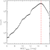 |
Fig. 1. Histogram of 144 831 057 ALLWISE WISE1 single-epoch measurements. A drop-off around 14.75 mag is shown by the red dashed line. |
The membership of the LMC was then determined by using the Gaia DR2 astrometric solution (Lindegren et al. 2018). Three Gaussian profiles, 1.805 ± 0.274 mas yr−1 for PMRA, 0.294 ± 0.442 mas yr−1 for PMDec, and −0.018 ± 0.068 mas for the parallax, were fitted to targets with errors < 0.5 mas yr−1 in proper motions (PMs) and < 0.5 mas in parallax as shown in Fig. 2. It is important to notice that for the parallax, except the Gaussian profile, an additional elliptical constraint was also applied where the primary and secondary radii of the ellipse were the 5σ limits of Gaussian profiles in PMRA and PMDec, respectively (see Fig. 4). Moreover, a constraint on the radial velocity (RV) ≥166.5 km s−1 was also applied for all targets having Gaia RV measurements as shown in Fig. 3. In total, this resulted in 197 005 targets. We note that by visually inspecting the Gaia color-magnitude diagram (CMD; see Fig. 5), there was an obvious outlier in the upper right region, which turned out to be a foreground star with RV = 39 km s−1. Even so, one out of 197 005 is an extremely small rate of contamination. After removing this target, we had a final sample of 197 004 sources as shown in Fig. 5, where a true distance modulus of 18.493 ± 0.055 mag for the LMC was adopted (same below; Pietrzyński et al. 2013). We note that the extinction correction was not applied when converting visual magnitudes into absolute magnitudes for convenience purposes since foreground extinction was relatively small at the line of sight of the LMC (AV ≈ 0.2 mag, if E(B − V)∼0.06 mag with the Galactic average value of RV = 3.1 was adopted; Oestreicher et al. 1995; Dobashi et al. 2008; Gao et al. 2013) and neither the internal extinction structure of the LMC nor the distance of the targets were accurately determined. In that sense, the internal extinction of the LMC might largely vary from star to star, especially for targets close to the star formation region (e.g., massive stars). Hence, the converted absolute magnitude only represents a lower limit for each individual star.
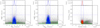 |
Fig. 2. Evaluation of the Gaia astrometric solution. Horizontal dashed lines indicate the limits of errors in PMs (0.5 mas yr−1) and parallax (0.5 mas). From left to right: Gaia PMs in Right Ascension, Declination, and parallax versus their errors are shown. Gaussian profiles were fitted in each panel and ±5σ were calculated (vertical dashed lines). For final selected targets (red) based on the parallax, except an adopted Gaussian fitting, an additional elliptical constraint was also applied with the 5σ limits of Gaussian profiles in PMRA and PMDec (based on blue targets in the first two panels), which are considered as the primary and secondary radii, respectively. Green contours show the number density in each diagram. |
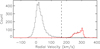 |
Fig. 3. Histogram of Gaia RVs. Milky Way and LMC are clearly separated. Selected targets (red) have a minimal value of ∼166.5 km s−1 (dashed line). |
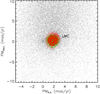 |
Fig. 4. PMRA versus PMDec diagram, for which the contamination of remaining foreground sources for the LMC is estimated around 0.08% (∼157/197 004) and can be ignored. Red dots indicate the astrometry constrained targets and green contours represent their number density. |
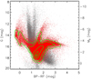 |
Fig. 5. GaiaG versus BP − RP diagram before (gray) and after (red) the astrometric constraints. A substantial amount of foreground contamination was removed. Green contours show the number density of astrometry constrained targets. |
Further evaluation of astrometric excess noise, which measures the disagreement and is expressed as an angle between the observations of a source and the best-fitting standard astrometric model (using five astrometric parameters), indicated that 98.17% and 99.78% targets had astrometric_excess_noise ≤ 0.5 and ≤1.0 mas, respectively. Moreover, Gaia Collaboration (2018b) provided lists of possible members based on the analysis of Gaia PMs and parallaxes for 75 Galactic globular clusters, nine dwarf spheroidal galaxies, one ultra-faint system, and the MCs. Their basic idea was to first determine the median and robust scatter in PMs and parallaxes by selecting a sample of stars covering a larger field of view, then further eliminate any sources showing larger scatter in the PMs, and finally construct a filter based on a covariance matrix of the cleaned sample, which allows one to properly deduce likely members. The comparison between our sample and Gaia Collaboration (2018b) indicates that 99.98% of our targets are consistent with their results. This suggests that our results are highly reliable without sophisticated correction (see more details and discussion in Sect. 2 of Yang et al. 2019).
Figure 4 shows PMRA versus PMDec. Based on this diagram, we estimated that the contamination of the remaining foreground and the possible nonpoint and background sources (SEIP sources without valid 2MASS measurements) for the LMC to be around 0.08% (∼157/197 004) and 0.5% (∼1034/197 004), respectively, and we determined that they could be ignored. In so doing, about 99.5% of our targets are most likely genuine members of the LMC.
After selecting the fiducial sample of 197 004 targets, we retrieved the following additional data (deblended with a search radius of 3″) by using a search radius of 1″ from different dataset ranging from the ultraviolet (UV) to far-infrared (FIR) as shown below (more details about each dataset can be found in Yang et al. 2019): 44 524 matches (∼23%) from the VISTA survey of the Magellanic Clouds system (VMC) DR4 (Cioni et al. 2011); 136 935 matches (∼70%) from the IRSF Magellanic Clouds point source catalog (MCPS; Kato et al. 2007); 37 116 matches (∼19%) from AKARI LMC point source catalog (Onaka et al. 2007; Murakami et al. 2007; Kato et al. 2012); 49 matches from HERschel Inventory of the Agents of Galaxy Evolution (HERITAGE) band-merged source catalog (units are in flux [mJy] instead of magnitude; Pilbratt et al. 2010; Meixner et al. 2013; Seale et al. 2014); 162 462 matches (∼82%) from SkyMapper DR1.1 (Keller et al. 2007; Bessell et al. 2011; Wolf et al. 2018); 151 476 matches (∼77%) from the NOAO source catalog (NSC) DR1 (Nidever et al. 2018); 20 379 matches (∼10%) from a UBVR CCD survey of the MCs by Massey (2002, M2002); 74 104 matches (∼38%) from Optical Gravitational Lensing Experiment (OGLE; Udalski et al. 1992, 2008, 2015; Szymanski 2005) Shallow Survey in the LMC (Ulaczyk et al. 2012); 215 matches from revised GALEX source catalog for the All-Sky Imaging Survey (GUVcat_AIS; Morrissey et al. 2007; Bianchi et al. 2017).
In total, there are 52 filters including two UV, 21 optical, and 29 IR filters. The spatial distributions of the additional optical (left) and IR (right) datasets are shown in Fig. 6 (GALEX and HERITAGE data are not shown in the diagram since the matches are scarce).
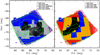 |
Fig. 6. Spatial distribution of the optical (left) and IR (right) datasets. |
The following additional classifications were also retrieved from the literature with a search radius of 1″, including: 113 matches from Whitney et al. (2008), for which ∼1000 young stellar objects (YSOs) and also some evolved stars were identified in the LMC based on their IR color and spectral energy distribution (SED); 143 447 matches from Boyer et al. (2011), who investigated the IR properties of cool, evolved stars in the MCs using observations from Spitzer; 124 matches from Jones et al. (2017), where nearly 800 point sources observed by the Spitzer Infrared Spectrograph (IRS; Houck et al. 2004) were classified using a decision tree method based on their infrared spectral features, continuum and SED shape, bolometric luminosity, cluster membership, and variability information; 98 matches from Massey & Olsen (2003), who used optical spectra to identify hundreds of RSGs in the MCs based on photometric data from Massey (2002); 620 matches from Bonanos et al. (2009), which is a catalog for 1750 massive stars in the LMC from the literature with accurate spectral types, and a multiwavelength photometric catalog for a subset of 1268 of these stars, with the goal of exploring their infrared properties; 63 matches from Neugent et al. (2012), who investigated the evolution of YSGs and RSGs in the LMC by identifying them based on the optical spectroscopy and comparing them with the new Geneva evolutionary models of the CMD; 108 matches from Evans et al. (2015), for which 263 massive stars in the northeastern region of the LMC were spectrally classified; 156 matches from González-Fernández et al. (2015), for which the physical properties of about 500 RSGs in the LMC and SMC were studied by using NIR/MIR photometry and optical spectroscopy; 31 919 matches from Simbad (Wenger et al. 2000). We retrieved RVs, optical spectral classifications, main object types, and auxiliary object types. Unmatched targets are most likely due to larger PMs, blends, or the photometric quality cuts.
As the foundation of our study, this multiwavelength source catalog with 197 004 targets ensures that we select genuine LMC members based on both astrometric and IR measurements. Figure 7 shows the histograms of magnitude distribution for each dataset (for convenience, the HERITAGE data are not shown here). Meanwhile, due to the huge amount of data required to be processed, we did not include the time-series data in our catalog. Any interested reader can retrieve the data by crossmatching our source catalog with the corresponding database. Our LMC source catalog of 197 004 targets is available in its entirety at CDS. Table 1 shows the content of each column of the catalog. Targets without errors indicate either a 95% confidence upper limit, or the errors are too large to be reliable (e.g., > 1.0 mag).
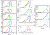 |
Fig. 7. Histograms of magnitude distribution in each dataset. The bin size of magnitude is 0.1 mag, except for the GALEX (0.5 mag) and AKARI (0.25 mag) data. For WISE3 and WISE4 bands, the histograms only show targets with S/N ≥ 10. For convenience, the HERITAGE data are not shown in the diagram. |
LMC source catalog contents.
3. Identifying evolved massive star candidates with the color-magnitude diagrams
To investigate evolved dusty massive stars, the first step is to identify them. However, for this paper, we decided to use modified color and magnitude cuts based on Yang et al. (2019) (see more details in Sect. 4 of Yang et al. 2019), which represent equivalent evolutionary phases (EEPs) from core helium burning to carbon burning with 7−40 M⊙ and AV = 1.0 mag (including both foreground and internal extinction), and they were scaled according to the LMC distance. It is important to take note that these cuts may not reflect the expected changes in the position of evolutionary features with metallicity. Using modified cuts instead of evolutionary tracks is mainly done when there is a problem (the EEPs do not properly fit the CMDs) with the models at LMC metallicity from Modules for Experiments in Stellar Astrophysics (MESA; Paxton et al. 2011, 2013, 2015, 2018) Isochrones & Stellar Tracks (MIST1; Choi et al. 2016; Dotter 2016) (A. Dotter, priv. comm.). Meanwhile, the PAdova and TRieste Stellar Evolution Code (PARSEC; Bressan et al. 2012; Tang et al. 2014; Chen et al. 2015, 2019) was also investigated. Unfortunately, the critical evolutionary points of PARSEC were also inappropriate for the data, plus the rotational mixing has not yet been introduced in PARSEC (Y. Chen, priv. comm.).
Firstly, Fig. 8 shows the comparison of Gaia CMDs between our sample and the LMC sample from Gaia Collaboration (2018b). We indicate the approximate positions of main sequence stars (MSs), blue helium burning stars (BHeBs; stars with initial masses ≥2 M⊙ and that evolved off the MS with core helium burning; Dohm-Palmer et al. 1997; McQuinn et al. 2011; Dalcanton et al. 2012; Schombert & McGaugh 2015), and red HeB stars (RHeBs) for the sample of Gaia Collaboration (2018b) (the BHeBs and RHeBs were referred to as BSGs and RSGs in our sample). From the diagram, it can be seen that since our sample was selected based on the infrared criterion (IRAC1 or WISE1 ≤ 15.0 mag), it presumably traces the relatively luminous, cooler evolved stars with a larger MLR, such as the BHeBs and RHeBs, than the MSs. Hotter stars, for example, most of the MSs, would not be selected due to the weaker radiation at the far end of the Rayleigh-Jeans tail and/or smaller MLR than the cooler evolved stars. However, there will inevitably also be a source of contamination from the main sequence massive stars at the blue end, which cannot be easily disentangled as shown in the diagram.
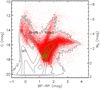 |
Fig. 8. Comparison of Gaia CMDs between our sample (red dots with green contours indicating the number density) and LMC sample from Gaia Collaboration (2018b) (gray contours indicating the number density). The approximate positions of MSs, BHeBs, and RHeBs for the sample of Gaia Collaboration (2018b) are indicated. |
Figure 9 shows multiple CMDs of Gaia, SkyMapper, NSC, OGLE, M2002, and 2MASS datasets. Each type of evolved massive star, namely BSGs (blue), YSGs (yellow), and RSGs (red), is indicated by the regions outlined by dashed lines. The criteria listed in Table 2 were determined based on Yang et al. (2019), but also modified according to the morphology of each population in the CMDs. That is to say, the determination was based on a bimodal distribution of the BSG and RSG candidates with a few YSG candidates lying between them. Moreover, even though the separation between RSGs and AGBs is relatively clear after the astrometric constraint (see Fig. 15 of Yang et al. 2019), as discussed in Sect. 3.1 of Yang et al. (2020), there is still a blurred boundary between RSGs and AGBs with continuity in photometry, variabilities, and even in their spectra. Currently, there is no efficient way to clearly distinguish between them. Thus, to be on the safe side, the red boundary of the RSG population was set by closely resembling the limit defined by the Cioni-Boyer method (Cioni et al. 2006; Boyer et al. 2011; Yang et al. 2019, 2020), which was bluer than the MIST boundary. It is important to notice that similar to the SMC (Yang et al. 2019), at the faint end of the RSG population (fainter than the limit of 7 M⊙ model track scaled from the SMC models), there is a distinct branch stretching continuously toward the TRGB after the astrometric constraint, indicating a genuine lower limit of initial mass of RSGs (6−7 M⊙), which is lower than the conventional definition (∼8 M⊙). However, in order to properly compare the result with the SMC and avoid further contamination from the red giants or AGBs, we did not set up a lower limit for the RSG population. We would also like to acknowledge that, up to now, almost no studies have focused on the faint end of the RSG population. For example, almost all of the spectroscopically confirmed RSGs in the SMC are brighter than KS ≈ 14.0 mag, which only represent ∼25% of the sample in Yang et al. (2020). Surprisingly, for our LMC sample, the percentage is even lower at ∼6% with almost all of the spectroscopically confirmed RSGs being brighter than KS ≈ 10.0 mag. In that sense, we barely have real knowledge about low-mass RSGs and the true difference between them and the AGBs. Moreover, some of the lowest-mass RSGs may temporarily exit the RSG phase, evolving to the left on the Hertzsprung-Russell diagram and producing a “blue loop” as they temporarily (or permanently) return to a YSG (or even BSG) state (Maeder & Conti 1994; Maeder & Meynet 2000; Meynet et al. 2015). Some of them may also be related to the intermediate-luminosity optical transients (ILOTs; Prieto et al. 2008; Bond et al. 2009; Berger et al. 2009). Thus, low-mass RSGs, connecting the evolved massive and intermediate stars, are crucial for understanding the star formation history and stellar evolution in nearby galaxies. More details and discussion can be found in corresponding sections of Yang et al. (2019, 2020). The average photometric uncertainties are indicated when available, while targets without errors are not shown in the CMDs.
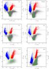 |
Fig. 9. Color-magnitude diagrams of Gaia (upper left), SkyMapper (upper right), NSC (middle left), OGLE (middle right), M2002 (bottom left), and 2MASS (bottom right) datasets. In each diagram, different regions of BSGs (blue), YSGs (yellow), and RSGs (red) are indicated by the dashed lines. The average photometric uncertainties are indicated when available. The diagrams show a clear bimodal distribution of the BSG and RSG candidates with few YSG candidates lying between them. |
Evolved massive star candidate selection criteria.
The candidates of each evolved massive star population were combined with duplicates were removed, resulting in 2974 RSG, 508 YSG, and 4786 BSG candidates in total as listed in Table 3. The candidates were then ranked (from 0 to 5) based on the intersection between different CMDs, where rank 0 indicates that a target has been identified as the same type of evolved massive star in all six datasets (Gaia, SkyMapper, NSC, M2002, OGLE, and 2MASS) and so on (we note that there is no rank 0 target for YSG candidates). The numbers of ranked candidates for each evolved massive star population are listed in Table 4. It also shows the comparison between the LMC and SMC, where the ranks are aligned based on the number of CMDs where a candidate has been identified as the same type of evolved massive star. Figure 10 shows Gaia and 2MASS CMDs for all ranked candidates which are color coded in red (RSGs), yellow (YSGs), and blue (BSGs) ranging from dark (rank 0) to light (rank 5). Detailed information about each type of evolved massive star candidate is presented in separate tables available at CDS, which has similar formats as Table 1. Finally, Fig. 11 shows the spatial distribution of evolved massive star candidates.
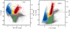 |
Fig. 10. Color-magnitude diagrams of Gaia (left) and 2MASS (right) with RSG (red), YSG (yellow), and BSG (blue) candidates overlapped, where the colors are coded from dark (rank 0) to light (rank 5) based on the ranks. The RSG branch extends toward fainter magnitudes with a few candidates scattered in the much fainter and redder region in the optical band, which is likely caused by the circumstellar dust envelope. Green contours represent the number density. |
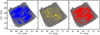 |
Fig. 11. Spatial distribution of BSG (left), YSG (middle), and RSG candidates (right). |
Numbers of identified evolved massive star candidates.
4. Comparison between the LMC and SMC
As the two source catalogs for the LMC and SMC are being established, we have an opportunity to compare the general properties of the two neighbor galaxies. However, it is also worth mentioning that these two catalogs only cover the main bodies of MCs since they are based on the observation of Spitzer. As a result, there will be more targets as well as evolved massive star candidates in the periphery of the MCs. A true distance modulus of 18.95 ± 0.07 mag for the SMC was adopted (Graczyk et al. 2014; Scowcroft et al. 2016), while the adopted extinction for selecting massive star candidates is the same as the LMC (AV = 1.0 mag; Yang et al. 2019). Figure 12 shows the multiple CMDs (MG versus BP − RP, MV versus B − V, MKS versus J − KS, MIRAC2 versus IRAC1 – IRAC2, MIRAC4 versus J – IRAC4, and MMIPS24 versus KS – MIPS24) from the optical to MIR for the source catalogs of the LMC (black) and SMC (gray). Massive star candidates are also overplotted and color coded in blue (BSGs), yellow (YSGs), and red (RSGs), with dark and light colors indicating targets from the LMC and SMC, respectively. It can be seen from the diagram that the most distinct difference between these two galaxies appears at the bright red end of the optical and NIR CMDs, where the cool evolved stars are located. The LMC targets, including RSGs, AGB, and RGs, are redder than the SMC ones, which is likely due to different metallicities or star formation histories (SFHs) between the two galaxies as discussed below.
 |
Fig. 12. Comparison of all targets in the LMC (black) and SMC (gray) in multiple CMDs of MG versus BP − RP (upper left), MV versus B − V (upper right), MKS versus J − KS (middle left), MIRAC2 versus IRAC1 − IRAC2 (middle right), MIRAC4 versus J – IRAC4 (bottom left), and MMIPS24 versus KS – MIPS24 (bottom right). Massive star candidates are color coded in blue (BSGs), yellow (YSGs), and red (RSGs), with dark and light colors indicating targets from the LMC and SMC, respectively. There is a prominent difference at the bright red end (RSG population) of the optical and NIR CMDs; this is illustrated by LMC targets which are shown in a redder color than the SMC ones. Meanwhile, this trend is reversed in the MIRAC2 versus IRAC1 – IRAC2 diagram with the LMC targets in a bluer color. |
Moreover, we also quantitatively compared the colors of massive star populations between these two galaxies as shown in Fig. 13. To be on the safe side, the comparison was only based on candidates selected in at least two CMDs (rank 0 to 4 in the LMC and rank 0 to 3 in the SMC). Targets were divided into equal magnitude bins (except the very bright end), for which the values of a median and standard deviation (SD) of color in each bin were calculated as summarized in Table A.1. It can be seen that there is almost no difference for the median values of BSG candidates between the LMC and SMC. The difference starts to emerge from YSG to RSG candidates, as LMC targets are getting redder, which may be due to the combined effect of several factors. One is that the average spectral type of RSGs moves toward earlier types at lower metallicities since the lower opacity leads to a higher effective temperature measured at a deeper layer of the stellar photosphere, and/or the metallicity-dependent Hayashi limit shifts to warmer temperatures at lower metallicities (Hayashi & Hoshi 1961; Elias & Frogel 1985; Massey & Olsen 2003; Levesque et al. 2006; Levesque & Massey 2012; Dorda et al. 2016). The other is that there is a positive relation between mass-loss rate (MLR) and metallicity (van Loon et al. 2005; Mauron & Josselin 2011), as a metallicity-scaling factor of (Z/Z⊙)0.7 may be applied to the de Jager et al. (1988) prescription which results in about 1.6 times higher MLR in the LMC than in the SMC. However, this difference is reversed in the IRAC1 − IRAC2 color (LMC targets are bluer than the SMC ones, the same as WISE1 − WISE2), which may indicate that there is a negative relation between CO absorption around 4.6 μm and the metallicity for RSGs. Moreover, the interaction between the MW, the LMC, and the SMC, which has triggered multiple peaks of star formation in the past few hundred million years (Yoshizawa & Noguchi 2003; Harris & Zaritsky 2009; Indu & Subramaniam 2011), may have a different effect on the two galaxies. For example, Bitsakis et al. (2017, 2018) studied the distribution and ages of star clusters in the LMC and SMC and found that the star clusters at the central regions were younger in the SMC than in the LMC. Therefore, if SMC RSGs are younger, then perhaps this may indicate that they have lost less mass, assuming the MLR is the same, so less material is around them. Thus they appear less red than the LMC ones.
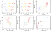 |
Fig. 13. Same as Fig. 12, but only for massive star candidates selected in at least two CMDs (rank 0 to 4 in the LMC and rank 0 to 3 in the SMC). For each diagram, targets are divided into equal magnitude bins and the values for the median (solid circles) and SD (errors) of color in each bin were calculated. |
We also converted the reddening-free color of (J − KS)0 (by adopting AV = 1.0 mag, AKS/AV ≈ 0.1, and AJ/AKS = 3.12; Wang & Chen 2019) of the massive star populations into the effective temperature (Teff) by using Eq. (3) of Yang et al. (2020) as shown in Fig. 14. As expected, the RSG population is located in a narrow range of about 3500 < Teff < 5000 K, the YSG population is around 5000 < Teff < 8000 K, and the BSG population is much broader as Teff > 8000 K. The difference in Teff between the LMC and SMC for each population also increases as ∼300 K for RSG, ∼1500 K for YSG, and more than ∼5000 K for the BSG population, respectively. However, we would also like to stress that the estimation of Teff for the hotter stars (e.g., BSGs) may suffer from larger uncertainties compared to cooler stars (e.g., RSGs) due to the weak emission at the NIR wavelength as discussed in the previous section.
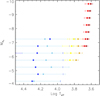 |
Fig. 14. Teff of massive star populations derived from reddening-free color of (J − KS)0. The Teff ranges are 3500 < Teff < 5000 K for the RSG population, 5000 < Teff < 8000 K for the YSG population, and Teff > 8000 K for the BSG population. Errors indicate the SD of the Teff. |
In addition, we would like to emphasize one important thing as mentioned in the previous section and also in Yang et al. (2019). Since our sample was selected based on the infrared criteria and constrained by multiple factors (deblending, astrometry, model limitation), hotter stars would be more incomplete than the cooler stars. Thus, the BSG to RSG ratio (B/R ratio) should not be simply assumed as ∼1.5:1 in the LMC or ∼1:1 in the SMC (e.g., see Table 4), since both the observation and theoretical prediction suggest more BSGs than RSGs (e.g., B/R ratio ∼4 or more) in the MCs (Meylan & Maeder 1982; Humphreys & McElroy 1984; Guo & Li 2002).
Numbers of ranked evolved massive star candidates in the LMC and SMC.
5. Summary
We present a clean, magnitude-limited (IRAC1 or WISE1 ≤ 15.0 mag) multiwavelength source catalog for the LMC. The catalog contains 197 004 targets with data in 52 different bands including two UV, 21 optical, and 29 infrared bands, which were retrieved from SEIP, VMC, IRSF, AKARI, HERITAGE, Gaia, SkyMapper, NSC, OGLE, M2002, and GALEX datasets, ranging from ultraviolet to far-infrared. Additional information about radial velocities and spectral and photometric classifications were collected from the literature.
The same method of Yang et al. (2019) was applied to establish the catalog, which was built by crossmatching (1″) and deblending (3″) between the SEIP source list and Gaia DR2 photometric data, with strict constraints on the PMs and parallaxes from Gaia DR2 in order to remove the foreground contamination. It was estimated that about 99.5% of the targets in our catalog were most likely genuine members of the LMC.
We compared our sample with the sample from Gaia Collaboration (2018b), indicating that the bright end of our sample was mostly comprised of BHeB and RHeB with inevitable contamination of MSs at the blue end. We applied modified magnitude and color cuts based on our previous works (Yang et al. 2019, 2020) on six different CMDs, and we identified 2974 RSG, 508 YSG, and 4786 BSG candidates in the LMC. The candidates were ranked according to the intersections among all available CMDs, for which those with the highest number (six) were given the highest rank.
The comparison between the source catalogs of the LMC and SMC indicates that the most distinct difference between these two galaxies appears at the bright red end of the optical and NIR CMDs, where the cool evolved stars are located. The LMC targets are redder than the SMC ones, which is likely due to the effect of metallicity and SFH. Meanwhile, the quantitative comparison of colors of massive star candidates in equal absolute magnitude bins shows that there is essentially no difference for the BSG candidates. However, there is an obvious discrepancy for the RSG candidates as LMC targets are redder than the SMC ones, which may be due to the combined effect of metallicity on both spectral type and MLR as well as the age effect. The Teff for massive star populations was also derived from the reddening-free color of (J − KS)0. The Teff ranges are 3500 < Teff < 5000 K for RSG population, 5000 < Teff < 8000 K for YSG population, and Teff > 8000 K for BSG population, with larger uncertainties toward the hotter stars.
Acknowledgments
We would like to thank the anonymous referee for many constructive comments and suggestions. This study has received funding from the European Research Council (ERC) under the European Union’s Horizon 2020 research and innovation programme (grant agreement number 772086). B.W.J and J.G. gratefully acknowledge support from the National Natural Science Foundation of China (Grant No.11533002 and U1631104). We thank Dr. Yang Chen for providing valuable comments on the stellar evolution models of PARSEC. This publication makes use of data products from the Two Micron All Sky Survey, which is a joint project of the University of Massachusetts and the Infrared Processing and Analysis Center/California Institute of Technology, funded by the National Aeronautics and Space Administration and the National Science Foundation. This work is based in part on observations made with the Spitzer Space Telescope, which is operated by the Jet Propulsion Laboratory, California Institute of Technology under a contract with NASA. This publication makes use of data products from the Wide-field Infrared Survey Explorer, which is a joint project of the University of California, Los Angeles, and the Jet Propulsion Laboratory/California Institute of Technology. It is funded by the National Aeronautics and Space Administration. This publication makes use of data products from the Near-Earth Object Wide-field Infrared Survey Explorer (NEOWISE), which is a project of the Jet Propulsion Laboratory/California Institute of Technology. NEOWISE is funded by the National Aeronautics and Space Administration. This research has made use of the NASA/IPAC Infrared Science Archive, which is operated by the Jet Propulsion Laboratory, California Institute of Technology, under contract with the National Aeronautics and Space Administration. This work has made use of data from the European Space Agency (ESA) mission Gaia (https://www.cosmos.esa.int/gaia), processed by the Gaia Data Processing and Analysis Consortium (DPAC, https://www.cosmos.esa.int/web/gaia/dpac/consortium). Funding for the DPAC has been provided by national institutions, in particular the institutions participating in the Gaia Multilateral Agreement. This research uses services or data provided by the NOAO Data Lab. NOAO is operated by the Association of Universities for Research in Astronomy (AURA), Inc. under a cooperative agreement with the National Science Foundation. The national facility capability for SkyMapper has been funded through ARC LIEF grant LE130100104 from the Australian Research Council, awarded to the University of Sydney, the Australian National University, Swinburne University of Technology, the University of Queensland, the University of Western Australia, the University of Melbourne, Curtin University of Technology, Monash University and the Australian Astronomical Observatory. SkyMapper is owned and operated by The Australian National University’s Research School of Astronomy and Astrophysics. The survey data were processed and provided by the SkyMapper Team at ANU. The SkyMapper node of the All-Sky Virtual Observatory (ASVO) is hosted at the National Computational Infrastructure (NCI). Development and support the SkyMapper node of the ASVO has been funded in part by Astronomy Australia Limited (AAL) and the Australian Government through the Commonwealth’s Education Investment Fund (EIF) and National Collaborative Research Infrastructure Strategy (NCRIS), particularly the National eResearch Collaboration Tools and Resources (NeCTAR) and the Australian National Data Service Projects (ANDS). This research has made use of the SIMBAD database and VizieR catalog access tool, operated at CDS, Strasbourg, France, and the Tool for OPerations on Catalogues And Tables (TOPCAT; Taylor 2005). Based on data products from observations made with ESO Telescopes at the La Silla or Paranal Observatories under ESO programme ID 179.B-2003.
References
- Adams, S. M., Kochanek, C. S., Gerke, J. R., et al. 2017, MNRAS, 468, 4968 [NASA ADS] [CrossRef] [Google Scholar]
- Berger, E., Soderberg, A. M., Chevalier, R. A., et al. 2009, ApJ, 699, 1850 [NASA ADS] [CrossRef] [Google Scholar]
- Bessell, M., Bloxham, G., Schmidt, B., et al. 2011, PASP, 123, 789 [NASA ADS] [CrossRef] [Google Scholar]
- Bianchi, L., Shiao, B., & Thilker, D. 2017, ApJS, 230, 24 [NASA ADS] [CrossRef] [Google Scholar]
- Bitsakis, T., Bonfini, P., González-Lópezlira, R. A., et al. 2017, ApJ, 845, 56 [NASA ADS] [CrossRef] [Google Scholar]
- Bitsakis, T., González-Lópezlira, R. A., Bonfini, P., et al. 2018, ApJ, 853, 104 [NASA ADS] [CrossRef] [Google Scholar]
- Bonanos, A. Z., Massa, D. L., Sewilo, M., et al. 2009, AJ, 138, 1003 [NASA ADS] [CrossRef] [Google Scholar]
- Bond, H. E., Bedin, L. R., Bonanos, A. Z., et al. 2009, ApJ, 695, L154 [NASA ADS] [CrossRef] [Google Scholar]
- Boyer, M. L., Srinivasan, S., van Loon, J. T., et al. 2011, AJ, 142, 103 [Google Scholar]
- Bressan, A., Marigo, P., Girardi, L., et al. 2012, MNRAS, 427, 127 [NASA ADS] [CrossRef] [Google Scholar]
- Cioni, M.-R. L., Girardi, L., Marigo, P., & Habing, H. J. 2006, A&A, 448, 77 [NASA ADS] [CrossRef] [EDP Sciences] [Google Scholar]
- Cioni, M.-R. L., Clementini, G., Girardi, L., et al. 2011, A&A, 527, A116 [NASA ADS] [CrossRef] [EDP Sciences] [Google Scholar]
- Chen, Y., Bressan, A., Girardi, L., et al. 2015, MNRAS, 452, 1068 [NASA ADS] [CrossRef] [Google Scholar]
- Chen, Y., Girardi, L., Fu, X., et al. 2019, A&A, 632, A105 [EDP Sciences] [Google Scholar]
- Choi, J., Dotter, A., Conroy, C., et al. 2016, ApJ, 823, 102 [Google Scholar]
- Crowther, P. A. 2019, Galaxies, 7, 88 [CrossRef] [Google Scholar]
- Dalcanton, J. J., Williams, B. F., Melbourne, J. L., et al. 2012, ApJS, 198, 6 [NASA ADS] [CrossRef] [Google Scholar]
- Davies, B., Kudritzki, R.-P., Plez, B., et al. 2013, ApJ, 767, 3 [NASA ADS] [CrossRef] [Google Scholar]
- de Jager, C., Nieuwenhuijzen, H., & van der Hucht, K. A. 1988, A&AS, 72, 259 [NASA ADS] [Google Scholar]
- Dobashi, K., Bernard, J.-P., Hughes, A., et al. 2008, A&A, 484, 205 [NASA ADS] [CrossRef] [EDP Sciences] [Google Scholar]
- Dohm-Palmer, R. C., Skillman, E. D., Saha, A., et al. 1997, AJ, 114, 2527 [NASA ADS] [CrossRef] [Google Scholar]
- Dorda, R., Negueruela, I., González-Fernández, C., & Tabernero, H. M. 2016, A&A, 592, A16 [NASA ADS] [CrossRef] [EDP Sciences] [Google Scholar]
- Dotter, A. 2016, ApJS, 222, 8 [NASA ADS] [CrossRef] [Google Scholar]
- Elias, J. H., & Frogel, J. A. 1985, ApJ, 289, 141 [NASA ADS] [CrossRef] [Google Scholar]
- Evans, C. J., Taylor, W. D., Hénault-Brunet, V., et al. 2011, A&A, 530, A108 [NASA ADS] [CrossRef] [EDP Sciences] [Google Scholar]
- Evans, C. J., van Loon, J. T., Hainich, R., et al. 2015, A&A, 584, A5 [NASA ADS] [CrossRef] [EDP Sciences] [Google Scholar]
- Gaia Collaboration (Brown, A. G. A., et al.) 2016a, A&A, 595, A2 [NASA ADS] [CrossRef] [EDP Sciences] [Google Scholar]
- Gaia Collaboration (Prusti, T., et al.) 2016b, 595, A&A, A1 [Google Scholar]
- Gaia Collaboration (Brown, A. G. A., et al.) 2018a, A&A, 616, A1 [NASA ADS] [CrossRef] [EDP Sciences] [Google Scholar]
- Gaia Collaboration (Helmi, A., et al.) 2018b, A&A, 616, A12 [NASA ADS] [CrossRef] [EDP Sciences] [Google Scholar]
- Gao, J., Jiang, B. W., Li, A., et al. 2013, ApJ, 776, 7 [Google Scholar]
- González-Fernández, C., Dorda, R., Negueruela, I., & Marco, A. 2015, A&A, 578, A3 [NASA ADS] [CrossRef] [EDP Sciences] [Google Scholar]
- Graczyk, D., Pietrzyński, G., Thompson, I. B., et al. 2014, ApJ, 780, 59 [NASA ADS] [CrossRef] [Google Scholar]
- Guo, J. H., & Li, Y. 2002, ApJ, 565, 559 [NASA ADS] [CrossRef] [Google Scholar]
- Harris, J., & Zaritsky, D. 2009, AJ, 138, 1243 [NASA ADS] [CrossRef] [Google Scholar]
- Hayashi, C., & Hoshi, R. 1961, PASJ, 13, 442 [Google Scholar]
- Houck, J. R., Roellig, T. L., van Cleve, J., et al. 2004, ApJS, 154, 18 [NASA ADS] [CrossRef] [Google Scholar]
- Humphreys, R. M., & McElroy, D. B. 1984, ApJ, 284, 565 [Google Scholar]
- Indu, G., & Subramaniam, A. 2011, A&A, 535, A115 [NASA ADS] [CrossRef] [EDP Sciences] [Google Scholar]
- Jones, O. C., Woods, P. M., Kemper, F., et al. 2017, MNRAS, 470, 3250 [NASA ADS] [CrossRef] [Google Scholar]
- Kato, D., Nagashima, C., Nagayama, T., et al. 2007, PASJ, 59, 615 [NASA ADS] [Google Scholar]
- Kato, D., Ita, Y., Onaka, T., et al. 2012, AJ, 144, 179 [NASA ADS] [CrossRef] [Google Scholar]
- Keller, S. C., Schmidt, B. P., Bessell, M. S., et al. 2007, PASA, 24, 1 [NASA ADS] [CrossRef] [Google Scholar]
- Levesque, E. M., & Massey, P. 2012, AJ, 144, 2 [CrossRef] [Google Scholar]
- Levesque, E. M., Massey, P., Olsen, K. A. G., et al. 2006, ApJ, 645, 1102 [NASA ADS] [CrossRef] [Google Scholar]
- Lindegren, L., Hernández, J., Bombrun, A., et al. 2018, A&A, 616, A2 [NASA ADS] [CrossRef] [EDP Sciences] [Google Scholar]
- Maeder, A., & Conti, P. S. 1994, ARA&A, 32, 227 [NASA ADS] [CrossRef] [Google Scholar]
- Maeder, A., & Meynet, G. 2000, ARA&A, 38, 143 [Google Scholar]
- Maeder, A., & Meynet, G. 2012, Rev. Mod. Phys., 84, 25 [Google Scholar]
- Massey, P. 2002, ApJS, 141, 81 [Google Scholar]
- Massey, P. 2013, New Astron. Rev., 57, 14 [NASA ADS] [CrossRef] [Google Scholar]
- Massey, P., & Olsen, K. A. G. 2003, AJ, 126, 2867 [NASA ADS] [CrossRef] [Google Scholar]
- Mauron, N., & Josselin, E. 2011, A&A, 526, A156 [NASA ADS] [CrossRef] [EDP Sciences] [Google Scholar]
- McQuinn, K. B. W., Skillman, E. D., Dalcanton, J. J., et al. 2011, ApJ, 740, 48 [NASA ADS] [CrossRef] [Google Scholar]
- Meixner, M., Panuzzo, P., Roman-Duval, J., et al. 2013, AJ, 146, 62 [NASA ADS] [CrossRef] [Google Scholar]
- Meylan, G., & Maeder, A. 1982, A&A, 108, 148 [NASA ADS] [Google Scholar]
- Meynet, G., Chomienne, V., Ekström, S., et al. 2015, A&A, 575, A60 [NASA ADS] [CrossRef] [EDP Sciences] [Google Scholar]
- Morrissey, P., Conrow, T., Barlow, T. A., et al. 2007, ApJS, 173, 682 [Google Scholar]
- Murakami, H., Baba, H., Barthel, P., et al. 2007, PASJ, 59, S369 [NASA ADS] [CrossRef] [MathSciNet] [Google Scholar]
- Neugent, K. F., Massey, P., Skiff, B., et al. 2012, ApJ, 749, 177 [NASA ADS] [CrossRef] [Google Scholar]
- Neugent, K. F., Levesque, E. M., Massey, P., et al. 2020, ApJ, 900, 118 [CrossRef] [Google Scholar]
- Nidever, D. L., Dey, A., Olsen, K., et al. 2018, AJ, 156, 131 [NASA ADS] [CrossRef] [Google Scholar]
- Oestreicher, M. O., Gochermann, J., & Schmidt-Kaler, T. 1995, A&AS, 112, 495 [NASA ADS] [Google Scholar]
- Onaka, T., Matsuhara, H., Wada, T., et al. 2007, PASJ, 59, S401 [Google Scholar]
- Paxton, B., Bildsten, L., Dotter, A., et al. 2011, ApJS, 192, 3 [Google Scholar]
- Paxton, B., Cantiello, M., Arras, P., et al. 2013, ApJS, 208, 4 [NASA ADS] [CrossRef] [Google Scholar]
- Paxton, B., Marchant, P., Schwab, J., et al. 2015, ApJS, 220, 15 [Google Scholar]
- Paxton, B., Schwab, J., Bauer, E. B., et al. 2018, ApJS, 234, 34 [Google Scholar]
- Pietrzyński, G., Graczyk, D., Gieren, W., et al. 2013, Nature, 495, 76 [NASA ADS] [CrossRef] [PubMed] [Google Scholar]
- Pilbratt, G. L., Riedinger, J. R., Passvogel, T., et al. 2010, A&A, 518, L1 [CrossRef] [EDP Sciences] [Google Scholar]
- Prieto, J. L., Kistler, M. D., Thompson, T. A., et al. 2008, ApJ, 681, L9 [NASA ADS] [CrossRef] [Google Scholar]
- Schombert, J., & McGaugh, S. 2015, AJ, 150, 72 [NASA ADS] [CrossRef] [Google Scholar]
- Scowcroft, V., Freedman, W. L., Madore, B. F., et al. 2016, ApJ, 816, 49 [NASA ADS] [CrossRef] [Google Scholar]
- Seale, J. P., Meixner, M., Sewiło, M., et al. 2014, AJ, 148, 124 [NASA ADS] [CrossRef] [Google Scholar]
- Skrutskie, M. F., Cutri, R. M., Stiening, R., et al. 2006, AJ, 131, 1163 [NASA ADS] [CrossRef] [Google Scholar]
- Smartt, S. J. 2009, ARA&A, 47, 63 [NASA ADS] [CrossRef] [Google Scholar]
- Smith, N. 2014, ARA&A, 52, 487 [Google Scholar]
- Szymanski, M. K. 2005, Acta Astron., 55, 43 [NASA ADS] [Google Scholar]
- Tang, J., Bressan, A., Rosenfield, P., et al. 2014, MNRAS, 445, 4287 [NASA ADS] [CrossRef] [Google Scholar]
- Taylor, M. B. 2005, ASP Conf. Ser., 347, 29 [Google Scholar]
- Udalski, A., Szymanski, M., Kaluzny, J., Kubiak, M., & Mateo, M. 1992, Acta Astron., 42, 253 [NASA ADS] [Google Scholar]
- Udalski, A., Szymanski, M. K., Soszynski, I., & Poleski, R. 2008, Acta Astron., 58, 69 [NASA ADS] [Google Scholar]
- Udalski, A., Szymański, M. K., & Szymański, G. 2015, Acta Astron., 65, 1 [NASA ADS] [Google Scholar]
- Ulaczyk, K., Szymański, M. K., Udalski, A., et al. 2012, Acta Astron., 62, 247 [NASA ADS] [Google Scholar]
- van Loon, J. T., Cioni, M.-R. L., Zijlstra, A. A., & Loup, C. 2005, A&A, 438, 273 [NASA ADS] [CrossRef] [EDP Sciences] [Google Scholar]
- Wang, S., & Chen, X. 2019, ApJ, 877, 116 [NASA ADS] [CrossRef] [Google Scholar]
- Wenger, M., Ochsenbein, F., Egret, D., et al. 2000, A&AS, 143, 9 [NASA ADS] [CrossRef] [EDP Sciences] [Google Scholar]
- Werner, M. W., Roellig, T. L., Low, F. J., et al. 2004, ApJS, 154, 1 [NASA ADS] [CrossRef] [Google Scholar]
- Whitney, B. A., Sewilo, M., Indebetouw, R., et al. 2008, AJ, 136, 18 [NASA ADS] [CrossRef] [Google Scholar]
- Wolf, C., Onken, C. A., Luvaul, L. C., et al. 2018, PASA, 35, e010 [Google Scholar]
- Woosley, S. E., Heger, A., & Weaver, T. A. 2002, Rev. Mod. Phys., 74, 1015 [NASA ADS] [CrossRef] [Google Scholar]
- Wright, E. L., Eisenhardt, P. R. M., Mainzer, A. K., et al. 2010, AJ, 140, 1868 [Google Scholar]
- Yang, M., & Jiang, B. W. 2011, ApJ, 727, 53 [NASA ADS] [CrossRef] [Google Scholar]
- Yang, M., & Jiang, B. W. 2012, ApJ, 754, 35 [NASA ADS] [CrossRef] [Google Scholar]
- Yang, M., Bonanos, A. Z., Jiang, B.-W., et al. 2018, A&A, 616, A175 [NASA ADS] [CrossRef] [EDP Sciences] [Google Scholar]
- Yang, M., Bonanos, A. Z., Jiang, B.-W., et al. 2019, A&A, 629, A91 [CrossRef] [EDP Sciences] [Google Scholar]
- Yang, M., Bonanos, A. Z., Jiang, B.-W., et al. 2020, A&A, 639, A116 [NASA ADS] [CrossRef] [EDP Sciences] [Google Scholar]
- Yoshizawa, A. M., & Noguchi, M. 2003, MNRAS, 339, 1135 [NASA ADS] [CrossRef] [Google Scholar]
Appendix A: Additional table
Color distribution of evolved massive star candidates between the LMC and SMC.
All Tables
Color distribution of evolved massive star candidates between the LMC and SMC.
All Figures
|
Fig. 1. Histogram of 144 831 057 ALLWISE WISE1 single-epoch measurements. A drop-off around 14.75 mag is shown by the red dashed line. |
| In the text | |
|
Fig. 2. Evaluation of the Gaia astrometric solution. Horizontal dashed lines indicate the limits of errors in PMs (0.5 mas yr−1) and parallax (0.5 mas). From left to right: Gaia PMs in Right Ascension, Declination, and parallax versus their errors are shown. Gaussian profiles were fitted in each panel and ±5σ were calculated (vertical dashed lines). For final selected targets (red) based on the parallax, except an adopted Gaussian fitting, an additional elliptical constraint was also applied with the 5σ limits of Gaussian profiles in PMRA and PMDec (based on blue targets in the first two panels), which are considered as the primary and secondary radii, respectively. Green contours show the number density in each diagram. |
| In the text | |
|
Fig. 3. Histogram of Gaia RVs. Milky Way and LMC are clearly separated. Selected targets (red) have a minimal value of ∼166.5 km s−1 (dashed line). |
| In the text | |
|
Fig. 4. PMRA versus PMDec diagram, for which the contamination of remaining foreground sources for the LMC is estimated around 0.08% (∼157/197 004) and can be ignored. Red dots indicate the astrometry constrained targets and green contours represent their number density. |
| In the text | |
|
Fig. 5. GaiaG versus BP − RP diagram before (gray) and after (red) the astrometric constraints. A substantial amount of foreground contamination was removed. Green contours show the number density of astrometry constrained targets. |
| In the text | |
|
Fig. 6. Spatial distribution of the optical (left) and IR (right) datasets. |
| In the text | |
|
Fig. 7. Histograms of magnitude distribution in each dataset. The bin size of magnitude is 0.1 mag, except for the GALEX (0.5 mag) and AKARI (0.25 mag) data. For WISE3 and WISE4 bands, the histograms only show targets with S/N ≥ 10. For convenience, the HERITAGE data are not shown in the diagram. |
| In the text | |
|
Fig. 8. Comparison of Gaia CMDs between our sample (red dots with green contours indicating the number density) and LMC sample from Gaia Collaboration (2018b) (gray contours indicating the number density). The approximate positions of MSs, BHeBs, and RHeBs for the sample of Gaia Collaboration (2018b) are indicated. |
| In the text | |
|
Fig. 9. Color-magnitude diagrams of Gaia (upper left), SkyMapper (upper right), NSC (middle left), OGLE (middle right), M2002 (bottom left), and 2MASS (bottom right) datasets. In each diagram, different regions of BSGs (blue), YSGs (yellow), and RSGs (red) are indicated by the dashed lines. The average photometric uncertainties are indicated when available. The diagrams show a clear bimodal distribution of the BSG and RSG candidates with few YSG candidates lying between them. |
| In the text | |
|
Fig. 10. Color-magnitude diagrams of Gaia (left) and 2MASS (right) with RSG (red), YSG (yellow), and BSG (blue) candidates overlapped, where the colors are coded from dark (rank 0) to light (rank 5) based on the ranks. The RSG branch extends toward fainter magnitudes with a few candidates scattered in the much fainter and redder region in the optical band, which is likely caused by the circumstellar dust envelope. Green contours represent the number density. |
| In the text | |
|
Fig. 11. Spatial distribution of BSG (left), YSG (middle), and RSG candidates (right). |
| In the text | |
|
Fig. 12. Comparison of all targets in the LMC (black) and SMC (gray) in multiple CMDs of MG versus BP − RP (upper left), MV versus B − V (upper right), MKS versus J − KS (middle left), MIRAC2 versus IRAC1 − IRAC2 (middle right), MIRAC4 versus J – IRAC4 (bottom left), and MMIPS24 versus KS – MIPS24 (bottom right). Massive star candidates are color coded in blue (BSGs), yellow (YSGs), and red (RSGs), with dark and light colors indicating targets from the LMC and SMC, respectively. There is a prominent difference at the bright red end (RSG population) of the optical and NIR CMDs; this is illustrated by LMC targets which are shown in a redder color than the SMC ones. Meanwhile, this trend is reversed in the MIRAC2 versus IRAC1 – IRAC2 diagram with the LMC targets in a bluer color. |
| In the text | |
|
Fig. 13. Same as Fig. 12, but only for massive star candidates selected in at least two CMDs (rank 0 to 4 in the LMC and rank 0 to 3 in the SMC). For each diagram, targets are divided into equal magnitude bins and the values for the median (solid circles) and SD (errors) of color in each bin were calculated. |
| In the text | |
|
Fig. 14. Teff of massive star populations derived from reddening-free color of (J − KS)0. The Teff ranges are 3500 < Teff < 5000 K for the RSG population, 5000 < Teff < 8000 K for the YSG population, and Teff > 8000 K for the BSG population. Errors indicate the SD of the Teff. |
| In the text | |
Current usage metrics show cumulative count of Article Views (full-text article views including HTML views, PDF and ePub downloads, according to the available data) and Abstracts Views on Vision4Press platform.
Data correspond to usage on the plateform after 2015. The current usage metrics is available 48-96 hours after online publication and is updated daily on week days.
Initial download of the metrics may take a while.