| Issue |
A&A
Volume 646, February 2021
|
|
|---|---|---|
| Article Number | A162 | |
| Number of page(s) | 34 | |
| Section | Planets and planetary systems | |
| DOI | https://doi.org/10.1051/0004-6361/202038839 | |
| Published online | 26 February 2021 | |
Internal water storage capacity of terrestrial planets and the effect of hydration on the M-R relation
1
Center for Space and Habitability, Gesellschaftsstrasse 6, Universität Bern,
3012
Bern,
Switzerland
2
Institute for Computational Science & Center for Theoretical Astrophysics and Cosmology, Universität Zürich,
Winterthurerstrasse 190,
8057
Zürich,
Switzerland
e-mail: This email address is being protected from spambots. You need JavaScript enabled to view it.
3
Institut für Geologie, Universität Bern,
Baltzerstrasse 3,
3012
Bern,
Switzerland
Received:
3
July
2020
Accepted:
4
December
2020
Abstract
Context. The discovery of low density exoplanets in the super-Earth mass regime suggests that ocean planets could be abundant in the galaxy. Understanding the chemical interactions between water and Mg-silicates or iron is essential for constraining the interiors of water-rich planets. Hydration effects have, however, been mostly neglected by the astrophysics community so far. As such effects are unlikely to have major impacts on theoretical mass-radius relations, this is justified as long as the measurement uncertainties are large. However, upcoming missions, such as the PLATO mission (scheduled launch 2026), are envisaged to reach a precision of up to ≈3 and ≈10% for radii and masses, respectively. As a result, we may soon enter an area in exoplanetary research where various physical and chemical effects such as hydration can no longer be ignored.
Aims. Our goal is to construct interior models for planets that include reliable prescriptions for hydration of the cores and mantles. These models can be used to refine previous results for which hydration has been neglected and to guide future characterization of observed exoplanets.
Methods. We have developed numerical tools to solve for the structure of multi-layered planets with variable boundary conditions and compositions. Here we consider three types of planets: dry interiors, hydrated interiors, and dry interiors plus surface ocean, where the ocean mass fraction corresponds to the mass fraction of the H2O equivalent in the hydrated case.
Results. We find H and OH storage capacities in the hydrated planets equivalent to 0−6 wt% H2O corresponding to up to ≈800 km deep ocean layers. In the mass range 0.1 ≤ M∕M⊕≤ 3, the effect of hydration on the total radius is found to be ≤2.5%, whereas the effect of separation into an isolated surface ocean is ≤5%. Furthermore, we find that our results are very sensitive to the bulk composition.
Key words: planets and satellites: composition / planets and satellites: oceans / planets and satellites: terrestrial planets / planets and satellites: interiors
© ESO 2021
1 Introduction
Water is abundant in the Universe; it is thought to have played an essential role in the onset of biochemistry on Earth and is indispensable for the sustainability of life as we know it (Kotwicki 1991; Kasting et al. 1993; Franck et al. 2001; Mottl et al. 2007; Jones et al. 2010; Güdel et al. 2014). These notions have led to a widely used definition of the classical habitable zone around a star. This zone is defined as the orbital region within which liquid water could exist on a planet’s surface in terms of the stellar flux it receives and assuming simple greenhouse effects mediated mainly by CO2 and H2O and maintained by the carbon cycle (Huang 1959; Rasool et al. 1970; Kasting et al. 1993; Kaltenegger et al. 2011; Ramirez 2018). This crude definition, although very useful as a first approach, cannot capture the full complexity of possible habitats as many other effects may be equally important for habitability. These include more diverse atmospheric compositions and chemical interactions, complex geochemical recycle processes, protection against harmful high energy particles from the host star via for example magnetic fields, and influences of the galactic neighbourhood (Ramirez 2018; Pierrehumbert et al. 2011; Gonzalez et al. 2001; Gonzalez 2005; López-Morales et al. 2011; Gallet et al. 2017; Javaux et al. 2010). Nevertheless, the presence of liquid water on a planet’s surface is still commonly used as a proxy to constrain the orbital region around a star where life could exist. Hence, water is of the utmost interest for both astrophysics and astrobiology and has attracted increasing attention from the planetary science community in recent decades (for example Kuchner 2003; Léger et al. 2004; Seager et al. 2007; Sotin et al. 2007; Noack et al. 2016, 2017; Alibert 2014, 2016; Fu et al. 2010; Kitzmann et al. 2015; Levi et al. 2017). It has been hypothesized that planets that formed beyond the ice line in the protoplanetary disk could migrate inwards into the habitable zone, where the accreted water ices would melt and form gigantic liquid surface oceans (Kuchner 2003; Léger et al. 2004). Indeed, in recent decades a large number of planets in the mass-range M ≲ 10 M⊕ have been detected with mean densities that are too low to correspond to a purely rocky composition (Rogers 2015; Lozovsky et al. 2018). These objects are not massive enough to have accreted substantial H-He envelopes in their past (Selsis et al. 2007; Sotin et al. 2007; Seager et al. 2007; Léger et al. 2004). This may suggest that their low densities are the results of extensive amounts of water on their surfaces. Such oceans could be maintained over timescales of several gigayears, long enough to allow for the emergence of life (Kuchner 2003; Noack et al. 2016). However, to sustain a biosphere, stable long-term climate conditions are required. For instance, it has been proposed by Laskar et al. (1993) that the stabilization of the Earth’s obliquity is crucial to avoid dramatic changes in climate that could have fatal consequences for life. These results were challenged later on by Lissauer et al. (2011), who found that the presence of a large moon has only a minor influence on the evolution of the obliquity fortimescales of hundreds of millions of years. Furthermore, Armstrong et al. (2014) found large variations of obliquity to even extend the outer edge of the habitable zone. Consequently, on Earth, long term climate stability is probably more strongly supported by a negative feedback mediated by the carbon cycle between the atmosphere and the mantle (Walker et al. 1981; Post et al. 1990; Kasting et al. 1993). The presence of such a geochemical cycle has often been assumed to be a requirement for the long term sustainability of life on other worlds as well. However, the interior dynamics of ocean planets could be quite different from those of water depleted planets like the Earth. It is still debated whether geochemical cycles, such as the carbon cycle, could be significant on water worlds. The mantles of these planets are expected to be isolated from the gas envelopes by liquid water layers and further shielded by high pressure ice layers at the bottom of the ocean. As a result, the presence of massive surface oceans could inhibit chemical transport mechanisms between the atmosphere and the interior (Alibert 2014; Kitzmann et al. 2015; Noack et al. 2016; Abbot et al. 2012; Wordsworth et al. 2013; Nakayama et al. 2019).
Apart from its astrobiological significance, water is also an important ingredient in many solar system bodies including the ice giants Uranus and Neptune and the icy satellites of Jupiter and Saturn. The exact role of water in internal processes and its distribution in the interiors of these objects are subjects of active research efforts and there are many remaining open questions. The interiorstructures of Uranus and Neptune, for instance, are still unknown (see review by Helled et al. 2020). A number of theoretical studies show that various structure models with different assumed compositions can match the gravitational moments measured by the Voyager 2 flybys (for example Helled et al. 2020 and references therein). These studies further suggest that it is possible that the ‘ice giants’ contain substantially lower ice to silicate ratios than is commonly assumed, and that their interiors could be rock dominated (Helled et al. 2011). Uranus could even have solar ice to rock ratios (Nettelmann et al. 2016). It is debated whether the rocks and ices are separated into differentiated layers or form a mixed interior with gradual composition gradients (Helled et al. 2011; Nettelmann et al. 2013). In the mixed case chemical interactions between the Mg-silicates in the mantle or the iron in the core and the water ices could be important factors in further constraining the composition and thermal profiles of these planets. However, such hydration effects in the interiors are generally not included in such studies. A detailed investigation of these aspects could significantly improve our understanding of the interiors of water rich solar system planets and would allow for a more reliable exoplanet characterization in the future.
In the context of exoplanets, interior characterization is aided by rather limited data. The planetary radii and masses along with some stellar properties are the primary parameters that are remotely accessible for planets outside the solar system. From these measurements it is possible to gain insight into their compositions and hence formation and evolution histories. Early efforts to link observed masses and radii with theoretical models for the interior compositions have been presented for example by Léger et al. (2004), Seager et al. (2007) and Sotin et al. (2007) over a decade ago. It is also worth noting the pioneering work by Zapolsky et al. (1969) long before the discovery of the first exoplanet. These authors have developed simple one-dimensional structure models to compute the total radii of planets as a function of mass, composition, and surface conditions. It has become common practice over the past years to use such models to interpret measured planetary masses and radii and predict possible interior structures and compositions. While such early approaches are quite powerful for inferring the general landscape of planetary properties, these models are highly degenerate. That is, many different internal compositions and profiles could match an observed M-R pair. This degeneracy has been noticed early on (for example Adams et al. 2007) and many researchers have devoted their work to minimize the possible parameter space for planetary interior properties for a given set of observed quantities (for example Rogers et al. 2010; Dorn et al. 2015, 2017; Grasset et al. 2009; Lozovsky et al. 2018). In these studies terrestrial planets are assumed to be fully differentiated into a number of compositionally distinct layers with water being modelled as an isolated surface layer. However, numerous studies over the past decades have shown that water can be incorporated in many minerals that are likely to be major constituents in the Earth’s mantle. The upper mantle mineral (Mg, Fe)2Si O4 (Olivine polymorphs) has been found to incorporate up to several wt% of water (see references in Tables E.1–E.3) in the correspondingly relevant temperature and pressure regime. At pressures ≈25–30 GPa, Ringwoodite (Rw), a high pressure polymorph of Olivine, dissociates into (Mg, Fe) O (Magnesiowüstite) and (Mg, Fe) Si O3 (Perovskite) (Wang et al. 1997). MgO can react with water to form Mg(OH)2 (Brucite) containing as much as ≈31 wt % H2O at moderate temperatures and pressures of ≲1500 K and ≲35 GPa (Hermann et al. 2016). Frost (1998) has determined the stability of the dense hydrous Mg-silicate Phase D and found it to be stable up to 50 GPa. This phase can incorporate up to 18 wt% of water. Nishi et al. (2014) have shown that Phase D transforms to an assemblage with another hydrous Mg-silicate, Phase H, at pressures above ≈ 48 GPa. Theyconcluded that this phase could transport water in the form of hydrates into the lowermost mantle. Furthermore, Perovskite, which is thought to play a minor role for water storage in the lower mantle of Earth (Inoue et al. 2010; Bolfan-Casanova 2005), transforms into post-Perovskite (pPv) between ≈100–130 GPa and remains stable up to ≈0.8−0.9 TPa (Umemoto et al. 2011), approximately the relevant pressure regime in the interiors of Uranus and Neptune. Although the hydration behaviour of pPv remains unknown, density-functional theory (DFT) simulations suggest that stable configurations containing at least 2–3 wt % water exist up to pressures of 150 GPa and possibly higher (Townsend et al. 2015). Finally, Silica (SiO2), which is stable over the entire pressure range relevant for the interiors of small to giant planets (Umemoto et al. 2011), has been reported to exhibit significant saturation contents of up to ≈ 3.2 wt % below 10 GPa and even up to ≈8.4 wt % for up to ≈100 GPa (Nisr et al. (2020) and references therein). In addition to the hydration of Mg-Silicates in the mantle, hydrogen solubility in the iron core might be equally important for constraining the total internal storage capacity of H2O equivalent in terrestrial planets. Indeed, it has been found that the solubility of hydrogen into iron is strongly enhanced at high pressures, relevant for the interiors of these objects (Fukai et al. 1983; Sugimoto et al. 1992). Although hydration effects under high pressure conditions have been actively studied by many researchers over the past decades, the bulk water content of the mantle remains one of the most poorly constrained compositional parameters of the Earth (Townsend et al. 2015; Cowan et al. 2014).
The effects of hydration on the equations of state of the core and mantle materials could affect the thermal profiles and total radii of the planets. More importantly, the capacity of storing large amounts of H and OH in planetary interiors could lead to the distribution of the total amount of water between an internal reservoir and a surface ocean. For an assumed total mass fraction of H2O equivalent this would mean that the surface ocean, and hence the pressure at the mantle-ocean interface, could be considerably smaller than one would expect on a fully differentiated planet. Indeed, Cowan et al. (2014) have derived steady-state solutions to the water partitioning between hydrosphere and mantle on terrestrial planets and find, based on simplified assumptions for the mineral hydration, that super-Earths tend to store large amounts of water in their interiors. This can have relevant implications for the results of previous studies. For example, Sotin et al. (2007) have presented a model that takes the atomic ratios of Mg, Si and Fe in the interior as input parameters to generate mass-radius relations for given surface conditions. Grasset et al. (2009) have used this model to quantify the effect of a surface water ocean on the total radius of a planet with given bulk composition. They inferred that bulk composition plays only a secondary role for the total radius in comparison to the effect of the ocean mass fraction. The authors estimated that if the planetary mass and radius are precisely known, it is possible to determine the total amount of water with a standard deviation of 4.5%. Alibert (2014) used a very similar model to compute the maximum radius of habitable planets assuming that habitability is hindered on water worlds by the formation of high pressure ice layers. It was concluded that for planets with 1–12 M⊕ this maximum radius is limited to 1.7–2.2 R⊕ and that larger planets are likely to be not habitable. These studies assume dry mantles and isolated surface oceans. However, in the light of the aforementioned hydration behaviour of Mg-silicates and iron, it is possible that these results are affected to a non-negligible extent when hydration is included. Understanding and quantifying these effects is essential given the increasing precision in mass and radius measurements for exoplanets. Although the mass and radius will never be precisely known, the uncertainties have decreased drastically over the past decades and will decrease further. To date, one of the most precise measurements of the radius of an exoplanet has been achieved for Kepler-93b (Ballard et al. 2014). Its radius has been determined from transit observations to with an uncertainty of approximately ± 1.3%. The PLATO mission, scheduled for launch in 2026, is expected to determine the radii and masses of terrestrial planets with precisions up to ≈3 and ≈10%, respectively (Rauer et al. 2016). Hence, second-order effects that were justified to be excluded in the past are expected to become necessary ingredients for future planetary characterization.
In this study we build upon the models presented by Sotin et al. (2007), Grasset et al. (2009) and Alibert (2014) and include the hydration of the mantle and the core as two separate reservoirs for H and OH and assess upper bounds for the corresponding effects on theoretical M-R relations. Furthermore, we apply our model to planets up to 3 M⊕ with simplified bulk compositions and show how the effects of hydration on M-R relations can be estimated. The mass limit of 3 M⊕ is dictated by the pressure range over which the core hydration model is valid. The generalization to more complex bulk compositions is briefly discussed.
This paper is structured as follows: in Sect. 2 we describe how the internal profiles of the planets are constructed for variable boundary conditions and compositions. In Sect. 3 we explain how the H and OH content in the Mg-silicates and the core is calculated as a function of pressure and temperature. The resulting estimates on the effect of hydration and differentiation on total planetary radii for different bulk compositions as a function of total planetary mass are discussed in Sect. 4. Caveats arising from some simplifying assumptions about the composition and hydration in our model are outlined in Sect. 5 and a summary of the work is provided in Sect. 6.
2 Planetary model
2.1 The structure equations
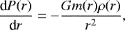
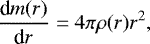
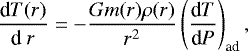
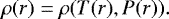
The internaltemperature, pressure, and density profiles need to be constructed to compute theoretical mass-radius relations. To this end the well known one-dimensional structure equations for spherical objects in hydrostatic equilibrium are integrated:
 (1)
(1)
 (2)
(2)
 (3)
(3)
 (4)
(4)
Here, P(r), T(r), ρ(r), and m(r) are the pressure, temperature, density, and enclosed mass at radial distance r, respectively, G is the gravitational constant and  is the adiabatic gradient. To compute the density as a function of pressure and temperature adequate equations of state need to be employed (see Appendix B). The hydration of the mantle and the core, hereafter referred to in terms of mass fraction
  or the molar hydrogen content ξH in the Mg-silicates and the iron is incorporated into the EoS (see Sect. 3).
The system of differential equations given by Eqs. (1)–(3) can readily be solved using a standard 4th order Runge-Kutta scheme with adaptive integration step size d r:
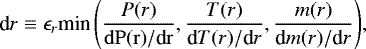 (5)
(5)
where ϵr is the refinement parameter. For an optimal trade off between stability and performance we recommend to use 0.1 ≤ ϵr ≤ 0.5. All results presented here have been obtained with ϵr = 0.25. The gradients have to be updated in each integration step to define the subsequent integration step size. With this procedure the planets are typically divided into a total of ~ 100−1000 individual shells. For simplicity, we set the water content  constant in each integration step. This induces a small error as P and T are of course different at the bottom of a shell and the top of the same shell. However, this effect can be controlled by the refinement parameter and can be neglected for our choice of ϵr.
2.2 Thermal model
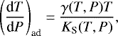
The adiabatic gradient in Eq. (3) is related to the material properties according to:
 (6)
(6)
where γ(T, P) and KS (T, P) are the Grüneisen parameter and the adiabatic bulk modulus, respectively. Equation (6) is commonly written in terms of the logarithmic temperature derivative ∇ad as:
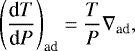 (7)
(7)
with
 (8)
(8)
The adiabatic bulk modulus can be related to the isothermal bulk modulus KT via the Grüneisen parameter γ and the thermal expansion coefficient αth using:
![Mathematical equation: \begin{equation*}K_{\textrm{S}}(P,T) = \left[1+\gamma(T,P) \alpha_{\textrm{th}}(T, P) T\right] K_{\textrm{T}}(T, P). \end{equation*}](/articles/aa/full_html/2021/02/aa38839-20/aa38839-20-eq12.png) (9)
(9)
KT and αth can be computed from the EoS (see Appendix B) directly:
 (10)
(10)
 (11)
(11)
The P and T dependance of the Grüneisen parameter can be expressed in terms of the density:
 (12)
(12)
In Eqs. (6)–(12), T and P are functions of the radial distance T(r) and P(r), which we have omitted to write explicitly for clarity. Equation (6) is only used for the iron in the core and the Mg-silicates in the mantle as for the pure water the adiabatic gradient  can self-consistently be extracted directly from the EoS used in this study (see Appendix B for details). The corresponding values for the Grüneisen parameter for the different layers are summarized in Table 1.
In the case of mixtures of N materials denoted by the index i the density is obtained using linear mixing:
 (13)
(13)
where Xi is the weight fraction of material i. The weight fractions are normalized to one, such that ∑iXi = 1. The isothermal bulk modulus and thermal expansion are then given by:
 (14)
(14)
 (15)
(15)
where we have omitted to write the T−P dependence of Xi for clarity. Here we do not account for composition gradients and hence the derivatives ∂Xi ∕∂P and ∂Xi ∕∂T vanish.
2.3 Composition
The model planets are composed of the elements Fe, Si, Mg, O and H. Minor elements such as C, Ni, Ca, S or Al are excluded since they would significantly increase the complexity of the composition beyond the scope of this study (see also Sotin et al. 2007). We point out that the presence of these elements could affect the hydration behaviour of the Mg-silicates and therefore change their water content (see also Sect. 5). Based on the assumed elemental composition the modelled objects are divided into two to four layers: a pure iron core, an upper and lower Mg-silicate mantle with variable Fe content and possibly a surface water ocean. The transition from the upper to the lower mantle is defined via the dissociation of Ringwoodite (Rw) into Magnesiowüstite (Mw) and Perovskite (Pv) occurring at ≈ 25−30 GPa (Wang et al. 1997):
 (16)
(16)
If the pressure at the bottom of the mantle does not exceed this transition pressure, only an upper mantle is present. We do not account for a possible differentiation of the core into a liquid and solid part and neglect the possible presence of lighter elements other than hydrogen in the core for simplicity.
For the purpose of illustrating how our model can be applied to estimate the water contents in planetary interiors, weimposed three simplifying assumptions: (1) the mantles of the modelled objects consist of pure  or
or  in the upper or lower mantle, respectively. The choice of these minerals was motivated by the fact that they are major constituents in the Earth’s mantle (Nunez-Valdez et al. 2013; Yao et al. 2012; Jacobsen 2006; Sinmyo et al. 2014; Li et al. 2014). Furthermore, Olivine (and its high pressure polymorphs) can incorporate considerable amounts of water and MgO can react with H2O to form Mg(OH)2 (see references inTable E.1–E.3 and also Sect. 3). (2) The minerals in the interiors of the hydrated planets are fully saturated. (3) Since higher Fe content in Olivine polymorphs generally leads to an increase in the water saturation level, we chose ξFe = 0.25 as it roughly marks the upper limit for which our hydration model is valid (see Sect. 3). We point out that, for the simplified bulk composition, the density in the lower mantle can be lower than in the upper mantle in the fully water saturated case if only little Fe is present. This is due to the high water storage capacity of ≈ 31 wt % in Brucite (Mg(OH)2 (Br)). This further motivates the choice of high Fe contents in the mantle. For our choice of ξFe this spurious behaviour could be avoided for all modelled cases and would naturally vanish in the Fe-free case if more Si-rich phases were present in the lower mantle.
In order to estimate the effects of hydration and ocean separation on M-R relations we consider here three types of planets: Dry planets (Type-1), hydrated planets (Type-2) and ocean planets (Type-3). The surface oceans are assumed to consist of pure water. An overview of the different types is provided in Fig. 1. The Type-1 planets have fully OH and H depleted interiors and no surface oceans. For the Type-2 planets the same boundary conditions, that is bulk composition and surface conditions, as for the Type-1 planets have been employed, but the mantles and cores are hydrated. A comparison between Type-1 and Type-2 planets allows for the assessment of the effect of hydration on total planetary radii. To estimate the effect of ocean differentiation we computed the amount of H2O equivalent in the Type-2 planets and added it as an isolated surface ocean on top of a dry mantle for the Type-3 planets. Since we are interested in estimating maximum effects in this study, intermediate cases where the water is partially distributed between an internal reservoir and a surface ocean, were not considered.
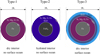 |
Fig. 1 Schematic overview of the different planet types modelled in this study. All objects consist of a pure iron or iron hydride coreand a dry or hydrated Mg-silicate mantle. We have estimated the effect of hydration by comparing the dry planets (Type-1) with their hydrated counterparts (Type-2) at fixed composition and boundary conditions. We have then extracted the water content in the Type-2 planets and moved it into an isolated surface layer (Type-3) to assess the effect of ocean separation on the total radius at fixed composition and boundary conditions. The oceans of the Type-3 planets can consist of an upper liquid part and a lower solid part if the pressure at the bottom of the oceans is high enough to allow for the formation of high pressure ices. |
2.4 Boundary conditions
After defining the compositions of the layers the interior structure was determined by integrating from the centre to the outermost layer using initial guesses for the central pressure PC and temperatureTC. For differentiated planets, the layer transitions must be assessed numerically using one of the integrated variables Q as a constraint, where Q is either the pressure, temperature, enclosed mass or radial extent of a layer or the total magnesium number of the planet. We used the core mass MCore to define the core mantle boundary (CMB) and the surface temperature TS to constrain the central temperature TC. The boundary conditions used in this study are: The total magnesium number Mg # ≡ [Mg]/([Mg] + [Fe]) including core and mantle, and the surface conditions PS, TS and M. The surfacepressure is automatically matched as it defines the surface of the planet. TS, M and Mg # were iteratively probed by adjusting TC, PC and MCore until the desired precision for the boundary conditions was achieved. Since these quantities are not independent, we employed the following prescription for predicting a new set of initial values S in each iteration:
 (17)
(17)
with
 (18)
(18)
 (19)
(19)
We found Eq. (17) to be sufficient in most cases to obtain the desired precision for all parameters and have hence omitted mixed terms in the Qi. In each iteration the coefficients aij are obtained by solving the following matrix equation for k, i = 0, 1, 2, 3 and j = 0, 1, 2:
 (20)
(20)
 (21)
(21)
 (22)
(22)
The subscript k refers to the kth data point that is needed to constrain all aij. In our case, four independent data points are required before the iterative prediction for the subsequent xkj can be carried out. These data points were obtained by roughly estimating the values Sj for a given set of boundary conditions Q from a pre-constructed grid and then adopting slight variations to the Sj. This procedure results in a very robust and efficient evaluation of the values Sj with very high accuracy for a given Q. In the case of hydrated planets, the hydrogen content in the core ξH is a priori unknown since it depends on the water content in the mantle and the temperature at the core mantle boundary (see Sect. 3.2 for details). However, as ξH is a required input for the FeHx EoS in the core, it must be estimated prior to the integration. Here, we treated ξH as a passive parameter in addition to the actively probed parameters Sj. In each iteration the two previous data points were used to predict the new value for ξH as a function of the new value for TC solely. With the procedure described above, ξH could be matched with high accuracy if TS was probed with sufficient accuracy. We note that in general a less sophisticated iteration scheme, where the values Sj are probed alternately via simple bisection, can be sufficient to achieve the same accuracy for the dry planets and the ocean planets. However, it failed for a considerable fraction of models for the hydrated planets. Furthermore, the procedure outlined above was found to be robust and more efficient than bisection. To determine when the quantity Qi has reached the desired precision we evoked the following criterion:
 (23)
(23)
where  is the desired precision for the parameter Qi. The same condition is used to probe the layer transitions using either the enclosed mass, the transition pressure or transition temperature as constraints. As the layer transitions in all our models depend on only one parameter, we probed the transition using simple bisection during the structure integration. The core-mantle transition has been probed using a fixed value for MCore, the upper-lower mantle transition via a fixed value for the dissociation pressure of Olivine, PUM→LM and the mantle-ocean transition using the enclosed mass M − MOcean at the bottom of the ocean. The corresponding values for the different parameters that have been used to define the boundary conditions and layer transitions are summarized in Table 2. We set higher accuracy for M of the Type-3 planets and TS of the Type-2 planets. This was necessary to achieve the desired precision for MOcean∕M and ξH, respectively. The transition criteria for the different layers are listed in Table 1. The specified accuracy was reached in about 80−90% of the modelled cases. For the rest of the planets the achieved accuracy for M, Mg #, ξH, and MOcean∕M were at least 10−3, 5 × 10⁻³, 3 × 10⁻², and 2 × 10⁻², respectively.These numerical uncertainties have, however, minor effect on the main results presented in this study. To obtain the mass-radius relations it is sufficient to vary the central pressure PC to cover a desired mass range. However, since we aim to compare different mass-radius curves directly we explicitly fixed M via PC for each of the modelled planets individually. This allows a direct comparison of the planetary properties for a given mass, composition, and surface conditions. In the case of dry mantles, where the composition in all layers is constant with depth, the core mass fraction can be computed analytically as a function of the total bulk and mantle compositions Mg # and ξFe, the total mass M and the ocean mass MOcean:
![Mathematical equation: \begin{equation*}\begin{split} \frac{M_{\textrm{Core}}}{M} = & \left( 1- \frac{M_{\textrm{Ocean}}}{M} \right)\left(\frac{1-\xi_{\textrm{Fe}}}{\textrm{Mg} \#}-1 \right) \\ & \times \left[ \xi_{\textrm{Fe}} \frac{ \tilde{m}}{m_{\textrm{Fe}}}+\frac{1-\xi_{\textrm{Fe}}}{\textrm{Mg} \#}-1\right]^{-1}, \end{split} \end{equation*}](/articles/aa/full_html/2021/02/aa38839-20/aa38839-20-eq31.png) (24)
(24)
where mFe the molar mass of iron.  is the mass of a portion of the material in the dry mantle containing one mole of Fe. It is defined as:
 (25)
(25)
The oxygen number O # is given by:
 (26)
(26)
The mantle mass fraction can then simply be computed for a given total mass and ocean mass fraction as MMantle = M − MCore − MOcean. In these cases the iteration for the core mass to match Mg # can be omitted. The core mass fractions and corresponding mantle mass fractions as a function of the mantle composition are plotted in Fig. 2 for different bulk compositions and ocean mass fractions.
For differentiated planets each individual layer can have a different convection behaviour based on the composition and the P − T-profiles. Hence, the heat transport via convection from the interior can be partially interrupted at a layer transition. This leads to a temperature drop upon transiting from a convective layer into a less convective one. Stixrude (2014) have presented models for the temperature profiles of super-Earths considering thermal regulation controlled by silicate melting. It was found that the temperature drop at the CMB denoted as ΔTCMB, can be represented by a simple scaling law as a function of the total planetary mass M:
 (27)
(27)
Here, weuse Eq. (27) to compute ΔTCMB over the modelled mass range and for all bulk compositions. We did not impose additional temperature jumps in the mantle transition zone (MTZ). We treat the temperature drop ΔTTBL in the thermal boundary layer (TBL) at the top of the Mg-silicate mantle (mantle-surface or mantle-ocean interface) as a free parameter and have considered values of 200, 700, 1200 and 1700 K. The value ΔTTBL = 1200 K roughly corresponds to modern day Earth with TS ≈ 300 K (for example Sotin et al. 2007). Since the water saturation in the mantle Mg-silicates drops with increasing temperature (see Sect. 3), the maximum effect at given composition and surface conditions is reached when the temperature discontinuity in the MTZ vanishes. We note, however, that a non-vanishing temperature jump in the MTZ could in principle increase the hydration of the iron core (see Sect.3.2). Furthermore, we only consider one value TS = 300 K because different values for TS could, in principle, be interpreted as different values for ΔTTBL. For instance, TS = 300 K and ΔTTBL = 1700 K could also be interpreted as TS = 800 and ΔTTBL = 1200 K. Furthermore, at elevated surface temperatures the definition of the Type-3 analogues would be less straightforward as part of the ocean mass fraction would enter the vapor phase. Since we do not account for atmospheres in this study, we explicitly fix TS = 300 K for the Type-3 planets.
In this study, we computed the mass-radius curves for fixed surface pressures and temperatures of PS = 1 bar and TS = 300 K. The Mg # has been varied between 0.2 and 0.7. This is roughly the range covered by estimates for elemental ratios of planet hosting stars presented by Grasset et al. (2009) (see their Fig. 2). We point out that for their presented value range of Mg/Si and Fe/Si, the magnesium number could be as high as ≈ 0.8. However, in this study Mg # must be strictly smaller than 1 − ξFe = 0.75 for the assumed Fe content in the mantles of ξFe = 0.25 if a core is present.
Layer properties.
Numerical precision for planetary parameters.
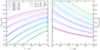 |
Fig. 2 Core mass fractions (left) and mantle mass fractions (right) as a function of the mantle composition ξFe according to Eq. (24) for different bulk compositions Mg # (colours) for MOcean∕M = 0 (solid), 0.05 (dashed), and 0.1 (dotted). |
2.5 Updating the shell contents
We assume the hydrogen content in the core to be homogeneous. For a given composition the water content in the mantle, however, is a function of temperature and pressure (and hence of radius). The water content was updated in each shell for the hydrous phases before integration according to the water storage capacity of the Mg-silicates (see Sect. 3). A change in the molar water content,  , leads to a change of the ratios Si/Mg. Therefore, in order to keep Si/Mg at a fixed value in each shell, the molar fractions of the different minerals need to be updated according to the water content. Here, this is irrelevant for the upper mantle since it consists of only one stoichiometry, the Olivine polymorphs, and hence its molar abundance, denoted by ξOl, is always equal to unity. In the lower mantle two minerals are present: Pv or pPv and Mw with molar Fe content ξFe. If water is added, the mole fractions of Pv or pPv and Mw ξPv and ξMw must be updated. The molar abundance of Mw is given by:
 (28)
(28)
The molar abundance of Pv/pPv is then simply given by:
 (29)
(29)
Here  is either 0 or (1 − ξFe)∕2, depending on the location in the phase diagram of Mg(OH)2 (see Sect. 3). For Pv/pPv we assume constant water content of 0.1 wt % (Pv) and 3.0 wt % (pPv) (see Sect. 3). We have assumed the hydrogen content in the core to be homogeneous with depth and hence ξH remains constant throughout the integration of the core.
2.6 Extracting the deep water reservoirs
2.6.1 In the core
The total amount of H2O equivalent in the core is given by the hydrogen content in FeHx, which is assumed to be homogeneous in the entire core. We discuss how the parameter x can be computed in Sect. 3.2. Once the stoichiometric hydrogen content x in the core is known, it can easily be converted toa molar abundance ξH as:
 (30)
(30)
The total atomic hydrogen content in the core is then given by:
 (31)
(31)
The H2O equivalent mass in the core can then easily be obtained:
 (32)
(32)
2.6.2 In the mantle
The local water weight fraction  in the mantle depends on the radial distance via P(r) and T(r). As outlined in Sect. 2.5, we assumed
  to be constant in each shell. The total mantle reservoir in a planet is then simply given by summation over all water containing shells. For a given shell, the water content
  was extracted from the shell properties using the following statement:
 (33)
(33)
where  and
and  are the molar amount of water in the shell and the molar mass of water, respectively.
  is related to the shell mass MShell and the molar water contents
  in the Mg-silicates (hereafter denoted as Mg-Si):
 (34)
(34)
with the relative molar masses given by:

Here, nMg-Si denotes the number of coexisting Mg-Si phases in the shell.  can directly be computed from
  by invoking mass balance:
![Mathematical equation: \begin{equation*}\xi_{\textrm{H}_2\textrm{O}, i}m_{\textrm{H}_2\textrm{O}} = X_{\textrm{H}_2\textrm{O}, i} \left[ (1-\xi_{\textrm{H}_2\textrm{O}, i}) m_{i} + \xi_{\textrm{H}_2\textrm{O}, i} m_{\textrm{H}_2\textrm{O}} \right] \end{equation*}](/articles/aa/full_html/2021/02/aa38839-20/aa38839-20-eq55.png) (37)
(37)
and hence:
 (38)
(38)
3 The hydration model
3.1 The mantle
Here we present a simple model for water saturation in Fe bearing Olivine polymorphs (upper mantle) and Brucite and Perovskite or post-Perovskite (lower mantle). We choose these minerals because they are known to be major constituents of the Earth’s mantle, where they are thought to play significant roles as hydrated Mg-silicates (see Sect. 2.3). The upper limit of hydration in the Mg-silicates is in general given by the saturation water content, which must be either measured in experiments or computed using molecular dynamics simulations. In an astrophysical framework, however, the extent of internal hydration of a planet cannot be assessed directly. That is, we cannot constrain it from stellar composition and total mass and radius alone. Thus, the water content in the mantle is written as  , where
 ![Mathematical equation: $\epsilon_{\textrm{H}_2\textrm{O}} \in [0, 1]$](/articles/aa/full_html/2021/02/aa38839-20/aa38839-20-eq58.png) is a free model parameter. It can be constrained from geophysical studies of terrestrial planets. Indeed, numerous authors have investigated the influence of water on the interior evolution of small objects and super-Earths and how the internal water content in mantle Mg-silicates evolves under the influence of a variety of geochemical and physical processes. For Mars, for instance, it has been shown that water loss from the interior over its evolution has been minor and that most of the initial water content in the mantle should still be present today (Hauck et al. 2002; Ruedas et al. 2013). Nakagawa et al. (2015) modelled water circulation mechanisms for the Earth and found that the water content in an initially anhydrous mantle increases over time as a result of hydration ofsubducting slabs. They found that a balance between regassing and degassing at shallow depths is reached, which dictates the total water content in the mantle. Nakagawa (2017) showed that in the case of strongly water-dependent viscosity water transport into the lower mantle is more effective, which can lead to higher internal water contents. Tikoo et al. (2017) modelled magma ocean solidification with variable initial water contents for the young Earth and showed that the water can be retained at saturation levels in the mantle upon cooling. Furthermore, Cowan et al. (2014) investigated water cycling between mantle and ocean and found that super-Earths tend to absorb more water in their mantles as the seafloor pressure is proportional to the surface gravity. These studies suggest that whenever a sufficient amount of water is present during planetary evolution, it is likely that the Mg-silicate mantle of the planet either remains or becomes strongly hydrated, which means
is a free model parameter. It can be constrained from geophysical studies of terrestrial planets. Indeed, numerous authors have investigated the influence of water on the interior evolution of small objects and super-Earths and how the internal water content in mantle Mg-silicates evolves under the influence of a variety of geochemical and physical processes. For Mars, for instance, it has been shown that water loss from the interior over its evolution has been minor and that most of the initial water content in the mantle should still be present today (Hauck et al. 2002; Ruedas et al. 2013). Nakagawa et al. (2015) modelled water circulation mechanisms for the Earth and found that the water content in an initially anhydrous mantle increases over time as a result of hydration ofsubducting slabs. They found that a balance between regassing and degassing at shallow depths is reached, which dictates the total water content in the mantle. Nakagawa (2017) showed that in the case of strongly water-dependent viscosity water transport into the lower mantle is more effective, which can lead to higher internal water contents. Tikoo et al. (2017) modelled magma ocean solidification with variable initial water contents for the young Earth and showed that the water can be retained at saturation levels in the mantle upon cooling. Furthermore, Cowan et al. (2014) investigated water cycling between mantle and ocean and found that super-Earths tend to absorb more water in their mantles as the seafloor pressure is proportional to the surface gravity. These studies suggest that whenever a sufficient amount of water is present during planetary evolution, it is likely that the Mg-silicate mantle of the planet either remains or becomes strongly hydrated, which means  . We are mainly interested in ocean planets that contain between a few and tens of wt% of water for which the condition of ‘sufficient’ amount of water is likely met. For the cases of lower water contents we still adopted
  to estimate the maximum possible effects of hydration. Therefore, whenever we refer to hydrated planets we shall assume fully water saturated Mg-silicates in the mantle, thatis
  , unless otherwise stated.
Our prescription for water saturation in Olivine polymorphs in the upper mantle is based on a collection ofexperimental data that has been acquired by various groups over the last decades. We construct a simple tri-linear model from a least squares fit to compute the saturation water content  as a function of temperature T, pressure P and iron content ξFe:
 (39)
(39)
A full list of the collected data that has been used for the fit, along with the corresponding references, is provided in Tables E.1–E.3 for the three different phase regions of  . The parameter range spanned by the data is T ≈ 1200−2400 K, P ≈ 0−30 GPa and ξFe ≈ 0−0.2. The fit has been performed such that the input parameters for Eq. (39) are T [K], P [GPa], ξFe [mol fraction] and the output is
  [wt fraction] (we note that these units are different from the original data set given in Tables E.1–E.3). The resulting set of fitting parameters for Eq. (39) are listed in Table B.4. We find that, to avoid overfitting, the coefficients c111 for all phases and c011 and c101 for the β- and γ-phase (for which the data sets are considerably smaller) have to be omitted. The same fit has been performed by omitting c011 and c101 also for the α-phase. However, since the water content in the α-phase spans a large range depending primarily on pressure and iron content, the effect of ξFe on
  is misrepresented at elevated pressures if c011 and c101 are excluded from the fit. Furthermore, at very high temperatures or very low pressures our fit can yield negative values for
  . We therefore invoke an artificial lower threshold value of
 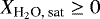 to avoid a non-physical behaviour.
In the lower mantle we chose Brucite (Mg(OH)2) and Perovskite (MgSiO3) as the waterbearing phases. We fix the water content in hydrous Perovskite at 0.1 wt % and neglect effects on the EoS for such low water contents (Inoue et al. 2010; Bolfan-Casanova 2005). For post-Perovskite it has been found that configurations containing more than 2 wt % of water are stable (Townsend et al. 2015). However, the pressure and temperature dependence of the water content has not been constrained. For this reason we adopt a constant value of 3 wt % (see also Appendix B.4). The stability field of Brucite is limited to rather low temperatures and pressures. It dissociates into MgO + H2O above ≈ 30−35 GPa (Hermann et al. 2016). We extracted the stability field of Mg(OH)2 in the P − T plane from Fig. 2 in Hermann et al. (2016). As a result, the lower mantle can itself be divided into two parts: an upper part where Mg(OH)2 is present and a lower part where only MgO is present.
3.2 The core
We assume that the main source of hydrogen that is dissolved in iron and eventually deposited into the core comes from the Mg-silicates and enters the iron via the reaction (Wu et al. 2018):
 (40)
(40)
In an early magma ocean hydrogen dissolves in liquid iron droplets and is incorporated into the core during the segregation process. If we assume that iron hydride, FeHx, droplets are in chemical equilibrium with the Mg-silicates at all times, then the hydrogen content in the iron is dictated by the conditions at the CMB. This notion allows us to compute the hydrogen content in the core by adopting chemical equilibrium between the core andthe lowermost mantle. If the water content in the mantle changes with time, either through external sources of water or the thermal evolution of the mantle, the hydrogen content in the core would adapt in order to maintain chemical equilibrium. Here we employ a simple model for the H-solubility as a function of the temperature at the CMB and the partial pressure of H2 in the lowermost part of the silicate mantle following Wu et al. (2018). These authors have used Sieverts’ law for gas solubility in metals to estimate the hydrogen concentration ξH in the iron cores of planetary embryos. We refer the interested reader to their Section 2.3 for further details. For our purpose it is sufficient to state the prescription for the hydrogen solubility in pure iron, which is given by:
![Mathematical equation: \begin{align*}\xi_{\textrm{H}} = \left(\frac{P_{\textrm{H}_2}}{P_0}\right)^{1/2} \cdot {\textrm{exp}} [(\Delta H^0 - T_{\textrm{CMB}} \Delta S^0)/RT_{\textrm{CMB}}], \end{align*}](/articles/aa/full_html/2021/02/aa38839-20/aa38839-20-eq70.png) (41)
(41)
where P0 = 1 bar is the reference pressure,  is the partial pressure of H2 in the silicates at the CMB, R is the universal gas constant and ΔH0 = +31.8 kJ mol−1 and ΔS0 = −38.1 kJ mol−1 K−1 are the enthalpy and entropy for dissolution of hydrogen into iron, respectively.
  is given by the amount of hydrogen present in the silicate mantle at the CMB. Here we used the van-der-Waals (VDW) EoS to relate the density of H2 to the partial pressure at given temperature. The Sieverts law is well suited to compute gas solubility in metals over an extended pressure range. However, Sugimoto et al. (1992) suggested that the Sieverts law underestimates the hydrogen solubility in iron at partial pressure
  GPa. Therefore, we restrict our study to planets with M ≤ 3 M⊕, which keeps
  strictly below ≈1.2 GPa for all modelled cases (see. Fig. 3).
4 Results and discussion
In the following we present the results for the total storage capacities of H2O equivalent (including core- and mantle reservoirs) in the mass range 0.1 ≤ M∕M⊕≤ 3 for differentbulk compositions, 1 bar surface pressure, 300 K surface temperature and ΔTTBL between 200and 1700 K. We also compare the different types of planets as described in Fig. 1 and estimate the net effect on thetotal radii as well as the internal density, pressure and temperature profiles. Finally, we discuss possible implications of our results to exoplanet characterization.
4.1 Water storage capacity and mass-radius relations
Here we address three main questions to illustrate the application of our model:
- 1.
What is the maximum amount of H2O equivalent that a terrestrial object of a given size, composition, and surface conditions can store in its interior?
- 2.
How different is the radius of such a hydrated object in comparison to its dry counterpart?
- 3.
How much does the radius change if the internal reservoir of H2O equivalent is moved into an isolated surface ocean?
To answer these questions we modelled three types of planets in the mass range 0.1 ≤ M∕M⊕≤ 3 by solving the structure equations for adequate boundary conditions (see Sect. 2 for details). An overview of the different types of planets is given in Fig. 1. We modelled a total of 1728 planets for four different values of ΔTTBL, six different Mg #, and twenty four values for M uniformly distributed in logarithmic space in the range 0.1 ≤ M∕M⊕≤ 3. Figures 4–6 show the central temperatures TC (first column), central pressures PC (second column) and the mass-radius relations (third column) obtained over the entire range of compositions and masses. The mass-radius relations for pure H2O, MgO and Fe at PS = 1 bar, TS = 300 K are also shown for reference. We find that while the central temperature changes significantly between the different types, the central pressure is relatively unaffected. This is because the adiabatic temperature gradient is steeper in hydrated Mg-silicates than in the anhydrous case, which leads to a net increase in the internal temperature profile for the Type-2 planets with respect to the Type-1 and Type-3 planets. Furthermore, Fig. 5 shows a slight change in the slope of the central temperature between ≈ 0.1 and 0.3 M⊕ corresponding to the positions of local maximum in the internal water content (see also discussion below and Fig. 7). Larger core mass fractions generally lead to larger central temperatures because the temperature gradient is steeper in the core than in the Mg-silicates. A similar behaviour is obtained for the central pressure. The central pressure decreases with Mg # for all planets because the pressure gradient is steeper in the core than in the Mg-silicate mantle (see also Sect. 4.2). That is, for a given surface pressure and total mass, increasing the core mass fraction (or equivalently decreasing Mg #) must be compensated by an increase in the central pressure. The local maximum of the total water content are also reflected in the curves for the central pressure by slight changes of the slope between ≈ 0.1 and 0.3 M⊕. The mass-radius relations are very similar for all planet types and show consistently larger radii for larger Mg # due to the lower density of the Mg-silicates with respect to the iron in the core. Furthermore, in Fig. 6 small kinks in the radius between ≈ 0.8 and 2 M⊕ are visible, corresponding to the Pv-pPv transition where the core reservoir in the Type-2 planets starts to increase drastically (see also next paragraph). This leads to a significant increase in the ocean mass fraction and hence reduction of the mean density in the Type-3 planets in the same mass range.
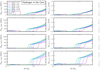 |
Fig. 3 Partial hydrogen pressure |


4.1.1 Comparison between Type-1 and Type-2 planets
In Fig. 7 we show the total water content (left column), the core- and mantle reservoirs (middle column) of the Type-2 planets and the resulting relative change in radius between Type-1 and Type-2 planets (right column). As expected, the fractional water content in the mantle increases strongly with the total Mg #. This is because larger mantle mass fractions have the effect of increasing the pressure range in the mantle, which leads to higher water saturation contents in Olivine polymorphs (see Fig. B.2). In addition, higher mantle mass fractions increase the amount of Mg-silicates with respect to the total planetary mass. Furthermore, the mantle reservoirs scale with the planetary mass only as long as an upper mantle is present. If the mass is sufficiently large that the transition pressure Ol →Pv + Mw is reached, more material from the lower mantle with lower water content is added. This is reflected in the distinct peaks in the total water content and the mantle reservoirs between 0.1 ≲ M∕M⊕≲ 0.3. The peak is highest for Mg# = 0.7 and ΔTTBL = 200 K at ≈ 3.8 wt% and decreases strongly for lower Mg# or higher ΔTTBL. In contrast, at higher masses the total water content is dominated by the core reservoir, which leads to an opposite trend. This is because the core reservoir scales with the core mass fraction and hence scalesinversely with the Mg #. The core reservoirs themselves exhibit local maximum between 0.1 ≲ M∕M⊕≲ 0.3 where the transition from the water rich upper mantle to the water poor lower mantle occurs. These maxima coincide with the local maxima in the mantle reservoirs (we note that this is only roughly true in the Fig. 7 because of the finite resolution of the curves). At higher masses 0.6 ≲ M∕M⊕≲ 2 the pressure at the bottom of the lower mantle exceeds the transition pressure between Pv and pPv leading to higher water contents in the Mg-Silicates at the CMB and hence higher equilibrium hydrogen content in the core. This is reflected in an increase in both core and mantle reservoirs for M ≳ 0.6−2 M⊕ and results in maximum total H2O equivalent reservoirs at 3 M⊕ of up to ≈3 wt% for ΔTTBL = 200 K and ≈6 wt% for ΔTTBL = 1700 K. The relative change in radius upon hydration is shown in the third column of Fig. 7 and exhibits three major trends:
First, independent of temperature, the effect of hydration on the mean density is always strongest roughly in the range 0.1 ≲ M∕M⊕≲ 0.3 where the mantle reservoirs peak despite the fact that for higher temperatures, the total fractional water content is much larger at higher masses. This means that hydration manifests more strongly for the upper mantle minerals than the iron core.
Second, the heights of the peaks clearly depend on ΔTTBL. Between 200 and 700 K the maximum δR1∕R1 decreases from ≈0.012 to ≈0.01, remains roughly constant between 700 and 1200 K and strongly increases between 1200 and 1700 K up to ≈ 0.025. To understand this behaviour several effects must be taken into account: (a) the water content in the upper mantle typically decreases with temperature. (b) The hydrogen content in the core increases with the water content in the upper mantle, provided there is no lower mantle. (c) The hydrogen solubility in the core increases with temperature. (d) Hydration tends to steepen the adiabatic temperature gradient leading to generally hotter interiors for the same boundary conditions, which increases the radius. Effects (a) and (b) lead to a decrease in the total fractional water content with temperature, which generally leads to a smaller change in the radius. Effect (c), on the other hand, leads to an increase in the total fractional water content with temperature. Hence, both effects (c) and (d) contribute positively to the relative change in radius while effects (a) and (b) have a negative contribution. The observed trend in the heights of the peaks therefore means that below 700 K effects (a) and (b) dominate while above 1200 K effects (c) and (d) are more profound. In the intermediate range between ~ 700 and 1200 K, the negative and positive contributions balance each other.
Finally, the third trend is that the Mg # for which δR1∕R1 is largest at given mass and temperature corresponds to the value of Mg # for which the total fractional water content is largest. Exceptions of this trend can beseen for ΔTTBL = 200 K below ≈0.8 M⊕. However, these small fluctuations are likely to have a numerical rather than a physical origin.
 |
Fig. 4 Central temperature (left column), central pressure (middle column), and M-R relation (right column) for the Type-1 planets. The different rows correspond to different assumed values for ΔTTBL (see annotations at the right). While the core temperature increases significantly for higher ΔTTBL the central pressure and radius remain vastly unaffected. The mass-radius relations for pure H2O, MgO and Fe are shown for reference. |
4.1.2 Comparison between Type-2 and Type-3 planets
The comparison of Type-2 and Type-3 planets is summarized in Fig. 8. The ocean mass fractions (middle column) for the Type-3 planets are calculated from the total water content in the Type-2 planets (compare first column in Fig. 7). The corresponding ocean depths are shown in the left column of Fig. 8. As expected, the ocean depths exhibit overall similar behaviour as the ocean mass fractions. But for lower masses a fixed ocean mass fraction results in generally lower ocean depths in comparison to the same ocean mass fraction at higher total mass. This is because  for spherical objects (see Appendix C for further discussion). We find that the estimated maximum H2O equivalent mass for all modelled planets corresponds to ocean layers with depths up to ≈ 800 km for M∕M⊕ = 3 and Mg # = 0.2. The effect of ΔTTBL on the ocean depth is twofold: higher temperatures reduce the water content in the mantle but can increase the core reservoir of the Type-2 planets (see Figs. B.2 and 3). Because the water content in the low mass planets is dominated by the upper mantles, this results in a downwards trend of the ocean depth with increasing ΔTTBL. Since
  in pPv is constant, at higher masses only the positive effect of ΔTTBL on the core reservoir manifests. This explains why the ocean depths scale upwards monotonously with temperature for M∕M⊕≳ 0.8 but not for lower masses. However, we remind the reader that the water content in pPv is in reality likely to change with P and T. A more realistic model for the hydration of pPv could therefore change the aforementioned behaviour.
The relative difference in radius δR2∕R2 ≡ (R3 − R2)∕R2 between the hydrated Type-2 planets and the fully differentiated Type-3 planets is in general larger than δR1 ∕R1 for a given mass. The maximum δR2∕R2 can reach up to ≈5% for M∕M⊕ = 3 and Mg # = 0.2. For temperatures ΔTTBL > 700 K the δR2∕R2 can in our model framework even become negative. This means, that differentiation into a surface ocean results in a net decrease in the planetary radius. Although counterintuitive at first glance, this feature does in fact arise intrinsically from the properties of the EoS used in this study. The temperature gradient in pure water tends to be shallower than in the hydrated silicates. As a result there is a considerable reduction of the interior temperature profiles between the Type-2 and Type-3 planets of up to a few thousand Kelvin (compare Figs. 5 and 6 or see Sect. 4.2). The densities of the cores and mantles of the Type-3 planets are hence enhanced due to the much lower temperatures and the absence of H or OH, respectively. For the 200 and 700 K planets, this effect is, however, very small, explaining why in this case all Type-3 planets are indeed inflated with respect to their Type-2 counterparts due to the presence of the low density surface ocean. At higher values of ΔTTBL the effect becomes large enough to counteract the decreasing effect on the mean density of the surface ocean. This can lead to a decrease in the total radius unless enough water is present. For large ocean mass fractions the decreasing contribution of the low density ocean dominates and the Type-3 planets are always larger than the Type-2 planets in the super-Earth regime. It is interesting to note that the change of sign of δR2 ∕R2 roughly lies at 1 M⊕ for solar composition (Mg# ≳ 0.5). This is because the Pv-pPv transition occurs at roughly the temperature and pressure conditions near the bottom of the Earth’s lower mantle.
Our findings indicate that the change in the total radius due to hydration is very likely below the detection limit of current or near future instrumentation for characterizing exoplanets. Furthermore, the maximum effect of hydration on the radius occurs in a mass range that is well below 1 M⊕. The partitioning of water between internal and surface reservoirs, on the other hand, can indeed affect a planet’s radius within plausible limits of observations in the foreseeable future. As this effect is enhanced for larger planetary masses, it is of particular interest for future characterization of planets in the super-Earth regime. However, here we used a relatively simple model for the hydration of the cores and mantles and have assumed a rather simple mantle composition. We discuss the limitations of our model in Sect. 5.
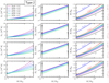 |
Fig. 5 Central temperature (left column), central pressure (middle column), and M-R relation (right column) for the Type-2 planets. The different rows correspond to different assumed values for ΔTTBL (see annotations at the right). While the core temperature increases significantly for higher ΔTTBL the central pressure and radius remain vastly unaffected. The central temperatures are strongly enhanced with respect to the Type-1 planets as the adiabatic gradient tends to get steepened by hydration. The mass-radius relations for pure H2O, MgO and Fe are shown for reference. |
 |
Fig. 6 Central temperature (left column), central pressure (middle column), and M-R relation (right column) for the Type-3 planets. The different rows correspond to different assumed values for ΔTTBL (see annotations at the right). While the core temperature increases significantly for higher ΔTTBL the central pressure and radius remain vastly unaffected. The kinks in the mass-radius curves correspondto the Pv-pPv transition, which leads to a drastic increase in the core reservoirs in the Type-2 planets. Accordingly, the ocean mass fractions in the Type-3 planets increase in the same mass range, which decreases the mean density of the palents. The mass-radius relations for pure H2O, MgO and Fe are shown for reference. |
4.2 Internal profiles
In Figs. 9–11 we show the internal temperature (left columns), pressure (middle columns), and density (right columns) profiles as functions of radial distance from the centre for three selected planetary masses. The solid, dashed, and dotted lines correspond to the Type-1, Type-2, and Type-3 analogues, respectively. The pressure profiles are very similar for all planet types. They are shifted to slightly lower pressures between Type-1 and Type-2 planets but are essentially indistinguishable by eye between Type-1 and Type-3 planets. The reason is the steeper pressure gradient in the core. As the mantle is hydrated, the ratio between total mantle mass (Mg-silicates plus water) and the core mass becomes larger. Therefore, for a fixed total mass and surface pressure, the central pressure needs to be reduced. Since the pressure difference in the surface oceans is very small in comparison to the central pressures nosimilar effect occurs between the Type-1 and Type-3 planets. The temperature profiles are much more sensitive to the model type and this sensitivity increases with increasing mass. The profiles shift to higher temperatures between Type-1/Type-2 planets. This is because hydration tends to steepen the temperature gradient in the mantle. Furthermore, the temperature profiles of the Type-1 and Type-3 planets are indistinguishable for 0.1 M⊕ but not for 0.6 M⊕ and 3 M⊕. The reason for this is that the oceans are very shallow at 0.1 M⊕ and become deeper for higher masses. As deeper oceans generally lead to larger temperature differences between the surface and the oceans, the internal temperature profiles at given surface temperature are more affected for deeper oceans (compare also Fig. 12). An interesting feature in Fig. 11 is that the temperature profiles in the Type-3 planets are higher for ΔTTBL = 200 K than even in the Type-2 planets. For higher values of ΔTTBL, however, the difference between the temperature profiles of the Type-3 planets and the Type-2 or Type-1 planets decreases. At very high temperatures the profiles of the Type-3 planets eventually fall even below the Type-1 planets. Considering the effect of the surface ocean on the temperature profiles alone cannot explain this behaviour. It would be intuitive to assume that larger oceans (larger temperature differences between surface and mantle) would monotonically increase the temperature in the mantle and the core. However, large ocean mass fractions also increase the pressure at the ocean-mantle interface. While the temperature gradient in the mantle becomes generally steeper for higher temperatures, it becomes shallower for higher pressures. For lower values for ΔTTBL the temperature effect dominates, rendering the temperature gradient steeper in the interior and hence resulting in somewhat higher temperature. For larger values of ΔTTBL, however, the pressure effect takes over, leading to a net decrease in the temperature gradient. The density profiles are very similar for all planet types. The density of the mantles and cores of the Type-2 planets are reduced compared to the Type-1 planets because of the hydration effects on the EoS. The Type-1 and Type-3 planets have, apart from the surface oceans, nearly identical density profiles.
Figure 12 shows the pressure at the bottom of the oceans (left column) and the temperature difference between the surface and the bottom of the oceans (right column) for Type-3 planets. The ocean pressures reach up to ~ 0.01−10 GPa where POcean ≳ 1 GPa is only reached for M ≳ 1 M⊕. This means that for the majority of the modelled objects the oceans are fully liquid (compare also Fig. B.1). For higher masses both the pressure and the temperature at the bottom of the ocean significantly increase. The temperature increase between the surface and the bottom of the ocean reaches up to ≈ 500 K, corresponding to temperatures at the bottom of the ocean of ≈800 K. The transition pressures from liquid water to the high pressure ices in the temperature range ≈ 300−800 K roughly lie in the range ≈1−10 GPa. This suggests that for larger masses the oceans of the Type-3 planets can posses an upper liquid layer and a lower solid layer (this is also evident in the density profiles shown in Fig. 11). These results indicate that the amount of H2O that can be stored in the interiors of terrestrial planets could reach up to ocean mass fractions sufficient for the formation of high pressure ice layers below the liquid parts of the oceans. This means, we find that large total water mass fractions of up to a few wt % could in fact easily be partitioned into interior and surface reservoirs so that the remaining surface oceans, that would in isolation be sufficiently large to form high pressure ice layers, would be liquid throughout. For low enough surface temperatures it is in principle also possible to have an ocean that is frozen throughout, regardless of the total ocean mass fraction. This scenario has, however, not been considered in this study.
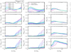 |
Fig. 7 Comparison between the Type-1 and Type-2 planets. Left column: total H2O equivalent in the interior assuming saturated Mg-silicates in the mantle and hydrogen content in the core computed from Sieverts law. Middle column: partitioning into separate contributions from the mantle- and core reservoirs. Right column: relative effect δR1 ∕R1 ≡ (R2 − R1)∕R1 of hydrationon total planetary radius at given mass, composition and surface temperature (see also Fig. 1). |
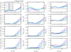 |
Fig. 8 Comparison between the Type-2 and Type-3 planets. Left column: depth of the surface oceans. Middle column: ocean mass fraction in the Type-3 planets. Of course,
|

4.3 Implications for previous studies
We have found that planets with considerable water content of at least a few wt % could still have only very small or no surface oceans. Thiscould have important implications in the context of previously published studies. The maximum radii for habitable planets derived by Alibert (2014), for instance, are likely to be underestimated. That is, the maximum total amount of H2O equivalent for which no high pressure ice layer forms at the bottom of the ocean could be considerably larger. This would lead to larger maximum radii for habitable planets.
Furthermore, our results could alter the findings of Grasset et al. (2009). These authors have estimated that the total ocean mass fraction could be derived from the bulk composition, the mass and the radius of a planet alone with a standard deviation of no more than 4.5% if the mass and radius were to be measured precisely. However, our study shows that the partitioning of the total water content into internaland surface reservoirs can have considerable effects on the radius of a planet. In particular, for super-Earths the partitioning between surface and internal reservoirs would decrease the total radius with respect to a fully differentiated ocean planet. That means that the mean density of such a planet would become more similar to the mean density of a fully water depleted planet and it becomes more difficult to distinguish between these objects. In this light, it has to be assumed that the determination of the water mass fraction present on an observed exoplanet from mass-radius measurements is less precise than suggested by Grasset et al. (2009).
5 Caveats
First, a number of simplifying assumptions for the bulk composition of the planets have been made (see Sect. 2.3). Including a larger variety of mantle minerals could induce a different overall hydration behaviour. For instance, Pyroxene plays a dominant role along with Olivine in the upper mantle of the Earth (Jacobsen 2006). The coexistence of different minerals can change the water content in the end member phases (Grant et al. 2006). Furthermore, SiO2 has been found to have large water storage capacity over a very wide pressure range and could be a major agent for water storage under lower mantle conditions. Nisr et al. (2020) have studied hydrous SiO2 samples up to ≈ 100 GPa and find water contents of 0.4−8.4 wt%. We have not included the possible presence of SiO2 in our models. In addition to the exclusion of some minerals that are thought to be important constituents in the Earth’s mantle, the hydration behaviour of some of the minerals are very weakly constrained. Most importantly, the saturation content in pPv is only poorly studied and to our knowledge, no data on the hydration behaviour as a function of pressure and temperature is currently available. The simplified assumption of constant water content of 3 wt % over the entire pressure and temperature range is likely to be unrealistic. The water content in pPv dictates the equilibrium hydrogen content in the core and is therefore a key parameter in our models and presumably one of the major sources of uncertainty at this stage.
These simplifying assumptions on the composition limit the interpretability of our results with respect to specific objects. For example, when assuming roughly solar [Fe]/[Mg] ≈ 0.5 for the bulk Earth, our results indicate that a maximum of ≈1.4 wt% of water could be stored in the Earth’s interior (see Fig. 7). This is much higher than standard estimates for the actual water content. From isotopic mass balance the total amount of water in the Earth’s interior at present is found to be ≈ 0.06−0.3 wt% (see review by Marty 2012). Geochemical and geophysical considerations lead to generally lower estimates for the mantle reservoirs of ≈ 0.006−0.07 wt% (see review by Ohtani 2019). Furthermore, Cowan et al. (2014) have developed simple two-box models for the water cycling between ocean and mantle and derived the internal water content of terrestrial planets based on the equilibrium between degassing and regassing. They reported a steady state solution for Earth with an internal water content of ≈ 0.08 wt%. One reason for the large discrepancy between our model and these results is, of course, the fact that we assumed water saturated Mg-silicates in the mantle. However, the Earth’s mantle is likely not fully water saturated (Ohtani 2019) and hence we do not expect our model to reproduce the actual water content but rather to give an upper limit. Another important factor is the fact that the ratio [Si]/[Mg] takes a fixed value of [Si]/[Mg] = 2/3 for our simplified composition. This is much lower than the solar value of [Si]/[Mg] ≈ 0.9 (Sotin et al. 2007). Adjusting the composition to roughly solar [Si]/[Mg] requires the inclusion of more Si-enriched phases in the mantle. We performed preliminary tests by adding dry (Mg, Fe)2Si2O6 to the upper mantle and increase the amount of (Mg,Fe)SiO3 in the lower mantle accordingly in order to increase the ratio [Si]/[Mg] to roughly solar. Furthermore, we have used a lower Fe content in the Mg-silicates of ξFe ≈ 0.1, which is thought to approximately represent the average Fe content in the Earth’s mantle (Sotin et al. 2007). Finally, to mimic the Earth as closely aspossible we adopted temperature discontinuities in the mantle transition zone (MTZ) at the top of the upper mantle of ΔTMTZ = 300 K (Sotin et al. 2007). With this the maximum water content for an Earth analogue decreases by about a factor of 5 to ≈0.28 wt%, in good agreement with the value range obtained from Marty (2012). However, since we ignored the hydration of Pyroxene for this preliminary test, the actual predicted value for the maximum water content in the Earth’s interior from our model would be somewhat higher. Furthermore, we have not included an SiO2 phase in the mantle composition, which could further increase the overall water storage capacity. In addition, the water content should be expected to be rather sensitive to ΔTMTZ and ΔTTBL as these parameters strongly affect the thermal profile in the mantle. These aspects indicate that the water content in the planetary interior is extremely sensitive to the bulk composition and the thermal state of the interior. Therefore, our model is suited for estimating the upper limits for the hydration effects for a given planetary mass and for Si/Mg = 2/3. Currently our model cannot be used to accurately predict the maximum water reservoirs in the interior of an object with a different composition. To this end, more diverse compositions need to be considered.
Second, in addition to excluding a number of mineral phases in the mantle that could play an import role for water storage, we also have not included possible effects on hydration of other elements s.a. C, Ni, Ca, S or Al. Various studies show, however, that water solubility can be rather sensitive to the incorporation of some of these elements. For example, Al has been found to affect the stability field of hydrous phases (Hermann et al. 2016) and could lead to the stability of hydrous phases up to higher pressures. It furthermore has been found to increase the water solubility in Olivine polymorphs and Pyroxene (Grant et al. 2006; Férot et al. 2012).
Accounting for more complex compositions as outlined above would also rise the question of how adequate our assumption of uniform composition in the mantle is (see Sects. 2.3 and 2.5). For example the Al content in Olivine is found to decrease significantly with increasing pressure and decreasing temperature (Férot et al. 2012). As the Al content can strongly influence the hydration behaviour, its pressure and temperature dependence might be an important factor. Similar issues could arise for the Fe content but has not been further investigated by the others at this point. However, we argue that the generalization to more complex compositions could inevitably lead to the necessity of allowing for composition gradients at least in the mantles of the planets. This would require a more sophisticated geochemical model for the phase assemblages as functions of pressure and temperature and the corresponding partitioning of water between the coexisting phases. We plan to address some of these topics in a subsequent study.
Third, our model is restricted to M ≤ 3 M⊕ due to the simple model for the chemical equilibrium between the core and mantle. As a result, for higher masses the partial hydrogen pressure in the lower parts of the mantle can exceed 1 GPa where the Sieverts law underestimates the hydrogen solubility in iron (Sugimoto et al. 1992). In the context of exoplanets, however, the super-Earth regime 1 ≲ M∕M⊕≲ 10 is of great interest. Therefore, it is desirable to employ more sophisticated chemical models in the future so the model can be extended to higher masses.
Fourth, we treated ΔTTBL and ξFe as free parameters. Furthermore, the estimate of ΔTCMB via Eq. (27) might not be universally applicable to planets of different sizes, compositions, and evolution histories. This renders these three aforementioned parameter as important sources of uncertainty. In Appendix A we present a brief sensitivity study of our model with respect to ξFe and ΔTCMB. Both parameters could have significant effects on the H and OH reservoirs and the resulting effects on the mean densities of the planets. In the super-Earth regime, the role of ξFe is difficult to estimate at this stage. This is because the effect of the iron content on the hydration behaviour of pPv could not be included in our model due to a lack of available data. Furthermore, the roles of pressure and temperature on the water content in pPv are, to our knowledge, not further constrained neither by experiments nor numerical simulations. However, the exact behaviour of  in pPv could significantly affect the predicted mantle and core reservoirs of super-Earths. We therefore emphasize the importance of further investigation of these minerals to allow more reliable predictions of internal H and OH reservoirs of terrestrial planets.
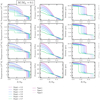 |
Fig. 9 Internal profiles as functions of radial distance from the centre for M∕M⊕ = 0.1 for all modelled ΔTTBL and compositions for the temperature (left column), pressure (middle column), and density (right). The solid curves correspond to Type-1 planets, the dashed curves to Type-2 planets and the dotted curves to Type-3 planets (see text for details). Since hydration tends to steepen the temperature gradient in the mantle, the Type-2 planets exhibit generally higher temperatures in the interiors than their Type-1 and Type-3 analogues. |
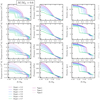 |
Fig. 10 Internal profiles as functions of radial distance from the centre for M∕M⊕ = 0.6 for all modelled ΔTTBL and compositions for the temperature (left column), pressure (middle column), and density (right column). The solid curves correspond to Type-1 planets, the dashed curves to Type-2 planets and the dotted curves to Type-3 planets (see text for details). Since hydration tends to steepen the temperature gradient in the mantle, the Type-2 planets exhibit generally higher temperatures in the interiors than their Type-1 and Type-3 analogues. |
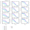 |
Fig. 11 Internal profiles as functions of radial distance from the centre for M∕M⊕ = 3 for all modelled ΔTTBL and compositions for the temperature (left column), pressure (middle column), and density (right column). The solid curves correspond to Type-1 planets, the dashed curves to Type-2 planets and the dotted curves to Type-3 planets (see text for details). Since hydration tends to steepen the temperature gradient in the mantle, the Type-2 planets exhibit generally higher temperatures in the interiors than their Type-1 and Type-3 analogues. For larger masses, the temperatureprofiles of the Type-3 planets can, however, exceed the temperature of the Type-2 planets for low values of ΔTTBL (see top row). |
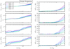 |
Fig. 12 Pressure at the bottom of the ocean (left column) and the temperature difference between the surface and the bottom of the ocean (right column). For large masses, the ocean mass is sufficient to reach pressures at the bottom of the oceans that exceed the transition pressure from liquid water to high pressure ices. This can also be seen in the density profiles in Fig. 11. |
6 Summary and conclusions
We have presented planetary structure models that account for the hydration of the Mg-silicate mantles and the iron cores. This allows for assessing the corresponding effects of water-interior interactions and ocean differentiation on the mass-radius relation and the partitioning of water between surface and internal reservoirs.
We considered three types of planets with simple bulk compositions (see Fig. 1): Dry planets (Type-1), hydrous planets (Type-2) and fully differentiated ocean planets (Type-3). For a first set of models we only considered Olivine polymorphs, Perovskite, Magnesiowüstit and Brucite in the mantle with a uniform Fe content of 25 mol%. The core-to-mantle mass ratio was derived from the total magnesium number Mg#, which is a free parameter. We then computed mass-radius curves for different bulk compositions at 300 K surface temperature and 1 bar surface pressure in the mass range M = 0.1−3 M⊕ and for different values for the temperature drop in the thermal boundary layer. Our main conclusions can be summarized as follows:
- 1.
The storage capacity of H2O equivalent in Type-2 planets is ≈ 0−6 wt% for 0.2 ≤Mg# ≤ 0.7 and M ≤ 3 M⊕. This corresponds to ocean depths in Type-3 planets of ≈0−800 km.
- 2.
The effect of hydration on the planetary radius peaks at ≈0.1−0.3 M⊕.
- 3.
The radii of super-Earths can be considerably smaller if water is stored in the interior instead of an isolated surface ocean.
- 4.
For the effects of hydration and ocean separation on the total radius, we find δR1∕R1 ≤ 2.5% and δR2∕R2 ≤ 5%, respectively.
- 5.
The temperature drop at the TBL has a great influence on the H and OH storage capacity and the resulting total radii.
- 6.
The results are very sensitive to the bulk composition and planet mass.
These results reveal the necessity of accounting for internal hydration for a more reliable characterization of the compositions and structures of exoplanets, in particular in the super-Earth regime. This will become even more essential with the increased precision of the mass-radius measurements that are expected in the near future. Here we have laid the foundations for further guiding the interpretation of observational data by incorporating these aspects into theoretical predictions of mass-radius relations.
Acknowledgements
This work has been carried out within the framework of the National Centre of Competence in Research PlanetS supported by the Swiss National Science Foundation. The authors acknowledge the financial support of the SNSF. We thank Morris Podolak and the anonymous referee for valuable comments.
Appendix A The sensitivity of the results to ΔTCMB and ξFe
In this section, we investigate the sensitivity of our results to the assumed temperature drop at the CMB (ΔTCMB) and the iron content in the Mg-silicates in the mantle (ξFe). We ran three comparison cases: ΔTCMB = 0.8ΔTCMB, nom, ΔTCMB = 1.2ΔTCMB, nom and ξFe = 0, where the subscript ‘om’ refers to the nominal case as presented in the main text. For simplicity, we only ran the bracketing cases of Mg# = 0.2, 0.7 and ΔTTBL = 200, 1700 K. ξFe is kept at the nominal value when ΔTCMB was changedand vice versa. Furthermore, the convergence criteria for the planets were somewhat relaxed as we only aim to give a rough estimation of the effects of these parameters.
Similarly to Figs. 7 and 8 of the main text, Figs. A.1–A.6 show the comparisons between the Type-1 and Type-2 planets and the Type-2 and Type-3 planets. The thick and thin curves correspond to the nominal and comparison cases, respectively. We find that changing ΔTCMB by ± 20% has a rather minor effect on the overall results.
The differences between the comparison and nominal cases are most prominent at higher masses where the core reservoir dominates. This is expected since for fixed surface conditions the temperature drop at the CMB predominantly affects the temperature in the core and not in the mantle. Therefore, the mantle reservoirs are rather unaffected by ΔTCMB. Furthermore, an increase or decrease in ΔTCMB leads to an increase or decrease in the hydrogen content in the core, which is consistent with Eq. (41).
The effects of ΔTCMB on δR1∕R1 are very weak while δR2∕R2 is shifted to slightly smaller/larger values for smaller/larger values of ΔTCMB for high masses and low Mg #. This indicates that ΔTCMB plays an important role for iron-rich super-Earths. The iron content in the mantle ξFe has a considerable effect on the main results, especially at lower masses, where the mantle reservoir dominates. This reflects the fact that the iron content in the mantle strongly influences the saturation water content in the upper mantle. If no iron is present in the mantle, the mantle reservoir is significantly decreased.
Furthermore, less iron in the mantle leads to larger cores at fixed bulk composition, which is reflected in slightly larger core reservoirs. In addition, the Pv-pPv transition is shifted to somewhat higher masses as the core to mantle ratio is enhanced for lower iron contents in the mantle. This is reflected in an offset of the core reservoirs between the nominal and the comparison case ξFe = 0. The effects on δR1∕R1 and δR2∕R2 are most prominent at lower masses and diminish at higher masses. It is still, however, unclear how reliably this behaviour reflects reality. This is because the water content in the lower mantle is intrinsically independent of ξFe in our model because no sophisticated model for the hydration of pPv could be employed. In reality, the water storage capacity in pPv could, however, very well be influenced by the iron content, which would render our results more sensitive to ξFe also at higher masses. These comparisons indicate that the iron content in the mantle is a crucial factor for determining internal H and OH reservoirs for low mass planets but its role is somewhat unclear for super-Earths at this stage.
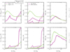 |
Fig. A.1 Comparison of the nominal case (thick curves) and ΔTCMB = 0.8 ⋅ ΔTCMB, nom (thin curves)for the bracketing cases Mg# = 0.2, 0.7 and ΔTTBL = 200, 1700 K. |
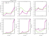 |
Fig. A.2 Comparison of the nominal case (thick curves) and ΔTCMB = 0.8 ⋅ ΔTCMB, nom (thin curves)for the bracketing cases Mg# = 0.2, 0.7 and ΔTTBL = 200, 1700 K. |
The opposite is true for ΔTCMB, which mainly affects the core reservoirs of super-Earths. In the context of exoplanets most of the observed terrestrial planets are in the super-Earth regime. For these planets both ΔTCMB and ξFe could play an important role for determining the internal H and OH reservoirs and corresponding effects of hydration and ocean differentiation on mass-radius relations.
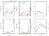 |
Fig. A.3 Comparison of the nominal case (thick curves) and ΔTCMB = 1.2 ⋅ ΔTCMB, nom (thin curves)for the bracketing cases Mg# = 0.2, 0.7 and ΔTTBL = 200, 1700 K. |
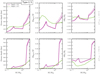 |
Fig. A.4 Comparison of the nominal case (thick curves) and ΔTCMB = 1.2 ⋅ ΔTCMB, nom (thin curves)for the bracketing cases Mg# = 0.2, 0.7 and ΔTTBL = 200, 1700 K. |
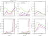 |
Fig. A.5 Comparison of the nominal case (thick curves) and ξFe = 0.0 (thin curves)for the bracketing cases Mg# = 0.2, 0.7 and ΔTTBL = 200, 1700 K. |
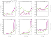 |
Fig. A.6 Comparison of the nominal case (thick curves) and ξFe = 0.0 (thin curves)for the bracketing cases Mg# = 0.2, 0.7 and ΔTTBL = 200, 1700 K. |
Appendix B Thermal equation of state
Here we describe in detail the equations of state used for the different materials in the core, mantle, and surface ocean. All results acquired in this study have been obtained using pre-generated EoS tables to optimize computational performance. We use piece-wise logarithmic spacing for both the temperature and the pressure axis, that is, we divided each decade into 10n grid points where we fixed n = 1 for all materials except for pure water where n = 2 was used. During the structure integration the corresponding parameters (s.a. ρ, KT or αth) at given P and T were extracted from the tables by bi-linear interpolation using the four adjacent grid points in the P − T-plane.
B.1 Dry and hydrous (Mg, Fe)2 SiO4
B.1.1 Phase transitions
(Mg,Fe)2 Si O4 exhibits three major polymorphic structures denoted by α-Ol, β-Ol and γ-Ol and hereafter generally referred to as Olivine polymorphs. To model the phase transitions of these phases, we performed linear fits from a set of experimental data for the transition pressure as a function of temperature (see Table E.4). The transition pressure is given as:
 (B.1)
(B.1)
The corresponding values for the fit coefficients a and b are given in Table B.5. These transitions depend on the Fe content in Olivine polymorphs and can be shifted by up to ≈0.5–2 GPa for Fe contents up to 25 mol%. The stability field of the γ-phase reaches up to at least ≈25 GPa and likely higher (Miyahara et al. 2011, 2016) and depends on the temperature. For simplicity we omit the effect of the Fe content on the phase transitions and assume a temperature independent stability field for γ-Ol up to 30 GPa to ensure that our prescription yields a strict upper bound for the water content. In light of the other simplifying assumptions for the composition (Sect.2.3) these approximations are justified. Furthermore, we point out that for super-Earths the mantles and hence the mantle reservoirs are dominated by the lower mantles. Therefore, the exact value for the dissociation pressure of Olivine becomes irrelevant for larger planetary masses.
B.1.2 Thermoelastic properties
In order to compute thermoelastic properties of water saturated Olivine polymorphs for different Fe contents ξFe relevant for planetary interior modelling an adequate EoS is required. A large number of studies have investigated in depth the EoS parameters for the anhydrous case and some efforts have been made to prescribe hydration effects on these parameters (see references in Tables E.1–E.3). The most commonly used analytical form of the EoS used in such studies is a third order Birch-Murnaghan equation. It relates the pressure P to the temperature T and the density ρ according to:
![Mathematical equation: \begin{align*}\begin{split} P(\rho, T) = & \frac{3}{2} K_{T,0}(T) \left[ \left(\frac{\rho(T)}{\rho_{T,0}(T)} \right)^{7/3} -\left(\frac{\rho(T)}{\rho_{T,0}(T)} \right)^{5/3}\right] \\ & \times \left(1 - \frac{3}{4}(4-K_{T,0}'(T)) \left[ \left(\frac{\rho(T)}{\rho_{T,0}(T)}^{2/3}-1\right) \right]\right). \end{split} \end{align*}](/articles/aa/full_html/2021/02/aa38839-20/aa38839-20-eq79.png) (B.2)
(B.2)
KT,0,  , and ρT,0 are the reference values for the bulk modulus, pressure derivative of bulk modulus and density at zero pressure. The reference bulk modulus and the reference density are functions of temperature and given by:
 (B.3)
(B.3)
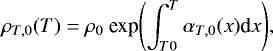 (B.4)
(B.4)
where ρ0 and K0 are the ambient density and the ambient bulk modulus (at P0 = 0 bar and T0 = 300 K). αT,0 is the isothermal expansion coefficient at zero pressure. It is expressed as:
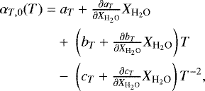 (B.5)
(B.5)
where we have adopted linear correction terms to account for hydration. Here we neglect the effect of Fe content on aT, bT and cT. Furthermore we do not account for any effects of Fe and water content on  . The reference parameters are computed following Mao et al. (2016) for the density and bulk modulus:
 (B.6)
(B.6)
 (B.7)
(B.7)
Here, ξFe and  are to be inserted in mole and weight fraction, respectively. The parameter values for Eqs.(B.3)–(B.5) used here are summarized in Table B.1 for the different phases along with the corresponding literature references. The coefficients for Eqs. (B.6) and (B.7) are listed in Table B.2.
Coefficients for density and bulk modulus of (Mg,Fe)2 Si O4 as a function of the water and Fe content from Mao et al. (2016).
EoS parameters for the different materials.
Fit coefficients for water saturation content in Olivine polymorphs.
Fit coefficients for phase transitions in Olivine polymorphs and Perovskite.
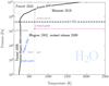 |
Fig. B.1 Phase diagram of pure water showing the four distinct EoS regions used in this study (thick black curves). The black, solid curve is the solid-liquid phase boundary above the triple point and the sublimation curve below the triple point. The black, dashed horizontal line shows the pressure where we switch from the low pressure EoS to the high pressure one. The high pressure ices (French et al. 2015) include ices VII and X. Other high pressure ice phases are not considered at this stage. The solid-liquid phase boundary is computed following Wagner et al. (2002) and French et al. (2016) for the low and high pressure regimes, respectively. |
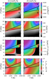 |
Fig. B.2 Phase diagrams of (Mg, Fe)2 Si O4. From top down: density, bulk modulus, saturation water content, and thermal expansion coefficient as functions of temperatureand pressure calculated from Eqs. (39) and (B.2). Shown are the Fe free case, that is ξFe = 0 (left) and ξFe = 0.25 (right). The dependence of the phase transitions on the Fe and water content are neglectedhere. The pressure and temperature range in the plot roughly marks the validity range of the model fit. We note that we have assumed a stability field of the γ-phase of up to ≲30 GPa, which overestimates the dissociation pressure of Ringwoodite. We imposed this assumption to ensure that our model yields strict upper bounds on the water content. |
All required parameters in Eq. (B.2) can then be computed as functions of water and Fe content. The density, bulk modulus, thermal expansion coefficient, and water saturation content  are plotted for the relevant P−T range in Fig. B.2 for ξFe = 0 (left panels) and for ξFe = 0.25 (right panels). In Sect. 3 we discuss how the saturation water content
  is computed.
B.2 Hydration model for Olivine polymorphs
The pressure in the compiled data set for water saturated Olivine polymorphs covers the entire stability range for each phase individually within the given temperature ranges. The latter is limited to the relevant regime for the Earth’s upper mantle (up to ≳ 2000 K). The colour maps in Fig. B.2 provide an overview of the density, bulk modulus, water content and thermal expansion for the Fe free case and for ξFe = 0.25. Theoverall effect of increasing temperature is a relatively strong decrease in the saturation water content  for all three phases. The water content reaches zero for T < 2500 K for all phases. This means that at higher temperatures the water content diminishes to zero and extrapolation to higher temperatures should therefore be unproblematic with regard to the hydration model. At low pressures P ≲ 5 GPa and high temperatures T ≳ 1500 K the fit predicts an increase in water content with temperature. This behaviour might not be physical. We point out that the experimental data do not reach temperatures below ≈1000 K. This is because they have been performed in the context of the Earth’s upper mantle for which temperatures between ≈ 1000 and 2000 K are relevant. Therefore, to model low values of ΔTTBL, it was inevitable to extrapolate to lower temperatures. It is, however, not clear how reliably the water content at such low temperatures is described by our model. Independent of the temperature, the model should be expected to yield unreliable results for Fe contents exceeding those covered by the data. Indeed, it can predict an increase in density upon hydration for ξFe ≳ 0.3 in the α-phase. At low temperatures (T ≲ 500 K), the model yields an increase in density upon hydration for the γ−phase above 25 GPa, which is clearly unrealistic. It is therefore strongly recommended to use the hydration model only for 0 ≤ ξFe ≲ 0.25 in general and at elevated temperatures (T > 500 K) if P ≳ 25 GPa.
B.3 Brucite
For Brucite (Br) we use experimental fits for the 3rd order Birch-Murnaghan EoS (Eqs. (B.2)–(B.5)). The correction terms  ,
,  , and
, and  vanish in these cases. The EoS parameters used in this study along with the corresponding references are summarized in Table B.3.
B.4 Perovskite, Periclase, and Wüstite
For Perovskite (Pv), Periclase (Per), and Wüstite (Ws) we use experimental fits for the Mie-Grüneisen-Debye EoS. In this case the pressure as a function of density and temperature is given as:
 (B.8)
(B.8)
Here, P(ρ, T0) is the non-thermal pressure contribution. It is identical to the non-thermal contribution of the Belonoshko EoS:
![Mathematical equation: \begin{align*}\begin{split} P(\rho, T) = & \frac{3}{2} K_{T,0}(T) \left[ \left(\frac{\rho(T)}{\rho_{T,0}(T)} \right)^{7/3} -\left(\frac{\rho(T)}{\rho_{T,0}(T)} \right)^{5/3}\right] \\ & \times \left(1 - \frac{3}{4}(4-K_{T,0}'(T)) \left[ \left(\frac{\rho(T)}{\rho_{T,0}(T)}^{2/3}-1\right) \right]\right). \end{split} \end{align*}](/articles/aa/full_html/2021/02/aa38839-20/aa38839-20-eq95.png) (B.9)
(B.9)
The ΔP denotes the thermal contribution to the pressure and is given as:
 (B.10)
where:
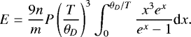 (B.11)
The Grüneisen parameter γ(T, P) at elevated temperatures and pressures is computed via Eq. (12). The Debye temperature is given as:
 (B.12)
The EoS parameters used in this study along with the corresponding references are summarized in Table B.3. We model (Mg,Fe)O (Magnesiowüstite) in the lower mantle as a mixture of MgO and FeO using linear mixing (Eq. (13)). For (Mg, Fe)SiO3 (Perovskite and post-Perovskite) we give the parameter values for the Fe free case in Table B.3. The effect of the Fe content on the thermoelastic properties is modelled by adjusting ρ0, K0, θD,0 and γ0. For ρ0 we taken the results for 3.8 mol% Fe and 6.1 mol% Fe from Sinmyo et al. (2014) for Pv. K0, θD,0, and γ0 are adjusted using the values for 13 mol% Fe from Wolf et al. (2015) and the Fe free values from Sun et al. (2018). The changes per mol % Fe of these parameters are then + 31 kg m−3, − 1.41 GPa, + 3.85 K, and − 0.0108, respectively. For pPv, the effect of Fe has been investigated by Shieh et al. (2005). However, comparing their results with the Fe free case from Sun et al. (2018) yields unrealistic results for Fe bearing pPv. For this reason we adopt the values from Pv above to model the Fe content in pPv. The transition pressure Ptrans(T) = aTransT + bTrans for Pv →pPv has been taken from Fig. 3 of Townsend et al. (2016) (see also Table B.5). Townsend et al. (2015) have found stable configurations of hydrous pPv containing at up to 2.31 wt % of water but have not investigated the saturation content as a function of pressure and temperature. Here we assume a constant maximum water content in pPv of 3 wt %.
B.5 Pure Fe and FeHx
For the iron in the cores of the modelled objects we proceed in analogy to Alibert (2014) and use the EoS fit to molecular dynamics calculations from Belonoshko (2010). It has a similar form than the 3rd order Birch-Murnaghan EoS but instead of the temperature dependance of K0,  and ρ0 an additional term is introduced to account for the thermal pressure:
![Mathematical equation: \begin{align*}\begin{split} P(\rho, T) = & P_{\textrm{th}}(\rho, T)\\ & + \frac{3}{2} K_0 \left[ \left(\frac{\rho(T)}{\rho_0} \right)^{7/3} -\left(\frac{\rho(T)}{\rho_0} \right)^{5/3}\right] \\ & \times \left(1 - \frac{3}{4}(4-K_0') \left[ \left(\frac{\rho(T)}{\rho_0}^{2/3}-1\right) \right]\right), \end{split} \end{align*}](/articles/aa/full_html/2021/02/aa38839-20/aa38839-20-eq100.png) (B.13)
(B.13)
with
 (B.14)
Here, γ is the Grüneisen parameter, given by Eq. (12), R the gas constant and m the molar mass of the modelled substance, here Fe. The EoS parameters are T0 = 300 K, K0 = 174 GPa,  , ρ0 = 8334 kg / m3, m = mFe = 0.0558 kg, γ0 = 2.434 and q = 0.489. The effect of the hydrogen content in FeHx on the EoS parameters of pure Fe are taken from Thompson et al. (2018). For convenience we rewrite FeHx = ξFeFe + (1 − ξFe)H where ξFe = 1 − ξH and ξH = x∕(1 + x). We then express the change of density and bulk modulus as:
 (B.15)
 (B.16)
To obtain the parameters d and k the change in density and bulk modulus between the pure Fe EoS and the values for FeHx from Table 2 in Thompson et al. (2018) have been fitted as linear functions of the pressure and the hydrogen content. From this we extracted the values d ≈−1620 kg m−3 and k ≈ −40.2 GPa. With this simple model fit the densities in Table 2 of Thompson et al. (2018) for low values of x, which are relevant for this study, can be reproduced with relative deviations of ≲1.2%. The hydrogen content in the core itself, x, is obtained from chemical equilibrium between the core and the Mg-silicate mantle and is discussed in more detail in Sect. 3.2.
B.5.1 Pure water
To model the most relevant phases of pure water in the surface oceans we employ different EoS for different P − T regions. At pressures below ≈1 GPa, the IAPWS formulation for liquid water (Wagner et al. 2002) and water ice Ih (Feistel et al. 2006) allow for as very reliable prescriptions of all relevant thermodynamic parameters. At higher pressures, where less or no experimental data are available, we switch to results obtained from molecular dynamics simulations. For the solid phase we use the thermodynamic potentials from French et al. (2015). Their fit includes water ices VII and X, which are the most important high pressure water ice polymorphs. The transition from low pressure ice Ih to the high pressure ices occurs at ≈ 0.2 GPa regardless of the temperature. Hence we switch from Wagner et al. (2002) to French et al. (2015) at 0.2 GPa. At high temperatures and pressures we switch tothe results of Mazevet et al. (2019). Their fit was performed such that it is consistent with the IAPWS at low pressures P ≲ 1 GPa. We switch from the IAPWS to Mazevet at 0.2 GPa. The transition between solid and liquid phases at all pressures are given by the water solidus. The solidus line is taken from Wagner et al. (2002) up to 1 GPa. For P > 10 GPa we take the results from French et al. (2016) and interpolate between 1 and 10 GPa. A summary of the phase diagram of pure water along with the EoS reference for each region used in this study is provided in Fig. B.1. For all phase regions the EoS is givenin the form of a thermodynamic potential. This allows computing the adiabatic gradient directly from the EoS using:
 (B.17)
where ρ, cP, P and αth are the density, specific isobaric heat, pressure, and thermal expansion. The isobaric heat is computed from the entropy:
 (B.18)
Appendix C Rough estimation of the ocean depth
Here we perform a very simple calculation to obtain a rough estimation on the behaviour of the ocean depth as a function of the total planetary mass for a fixed ocean mass fraction. Using the fact that for spherical objects we have  , we express the ocean mass fraction MOc∕M as:
![Mathematical equation: \begin{align*}\frac{M_{\textrm{Oc}}}{M} = \frac{[(R_0+R_{\textrm{Oc}})^3-R_0^3]\left< \rho_{\textrm{Oc}}\right>}{R_0 ^3 \left< \rho_0 \right>}, \end{align*}](/articles/aa/full_html/2021/02/aa38839-20/aa38839-20-eq108.png) (C.1)
(C.1)
where R0 denotes theradius of the solid planet (iron core + silicate mantle) and ROc denotes the ocean depth as measured from R0. Using the first order Taylor expansion  we can approximate MOc∕M for ROc∕R0 ≪ 1 as:
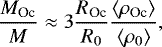 (C.2)
(C.2)
and hence:
![Mathematical equation: \begin{align*}R_{\textrm{Oc}}(M, M_{\textrm{Oc}}) \approx \frac{1}{3} \left(\frac{3}{4 \pi} \left[ 1- \frac{M_{\textrm{Oc}}}{M}\right]\frac{M}{\left< \rho_0 \right>}\right)^{1/3} \frac{M_{\textrm{Oc}}}{M} \frac{\left< \rho_0\right>}{\left< \rho_{\textrm{Oc}} \right>}. \end{align*}](/articles/aa/full_html/2021/02/aa38839-20/aa38839-20-eq111.png) (C.3)
(C.3)
Equation (C.3) is plotted for different ocean fractions MOc∕M in Fig. C.1 and assuming  and
and  , which roughly corresponds to the values for an earth like planet. Of course, the densities would be strongly dependant on the bulk composition and the total mass of the planet.
  and
and  could, in principle, be obtained from fits to our data. However, here we are merely interested in an order of magnitude estimation and the overall behaviour of the ocean depth as a function of the total mass. Figure C.1 shows a clear upwards trend of the ocean depth with total planetary mass at given ocean mass fraction. Hence, the fact that the same ocean mass fraction produces a deeper ocean for a higher total mass than for a lower total mass in Fig. 8 can qualitatively be explained by Eq. (C.3).
Appendix D Sensitivity of ρ
to  and
and 
To computethe isothermal expansion coefficient at zero pressure in Eq. (B.5) we introduced linear correction terms to account for hydration effects. The corresponding coefficients  and
and  have been estimated by extrapolating existing data (Ye et al. 2009). The uncertainty on these parameters are hence likely to be large and it is hence required to assess the sensitivity of our model to these parameters. We computed the effect on the density of saturated Olivine by varying
  and
and  by ± 50%. We find the density to be changed by up to ≈4−6% for temperatures between ≈1000 and 1500 K and ≈0−2% else. The enhanced sensitivity between ≈1000 and 1500 K comes from the fact that our hydration model is most sensitive to the water content in this regime. On one hand higher temperatures lead to lower water contents but at the same time stronger sensitivity to the water content according to Eq. (B.5). These two effects counteract each other and the resulting net effect is strongest between ≈ 1000 and 1500 K. This implies that more refined assessments of the hydration effects on Mg-silicates from experiments or first-principle simulations is crucial for obtaining reliable results from our model. However, for masses M∕M⊕≳ 0.3 the upper mantle contributes lesser to the overall structure the more massive the planets get and hence the sensitivity to
  and
and  can be safely neglected for super-Earths. Furthermore, as for higher temperature profiles in the mantles, that is larger values of ΔTTBL, the water content in the upper mantle diminishes the contribution of these parameters diminish.
Appendix E Data tables
Saturation water content in α−(Mg,Fe)2 Si O4.
Saturation water content in β−(Mg,Fe)2 Si O4.
Saturation water content in γ−(Mg,Fe)2 Si O4.
Phase transition data for anhydrous Mg2Si O4.
References
- Abbot, D. S., Cowan, N. B., & Ciesla, F. J. 2012, ApJ, 756, 178 [NASA ADS] [CrossRef] [Google Scholar]
- Adams, E. R., & Seager, S. 2007, ApJ, 673, 1160 [Google Scholar]
- Alibert, Y. 2014, A&A, 561, A41 [NASA ADS] [CrossRef] [EDP Sciences] [Google Scholar]
- Alibert, Y. 2016, A&A, 591, A79 [NASA ADS] [CrossRef] [EDP Sciences] [Google Scholar]
- Armstrong, J. C., Barnes, R., Breiner, J., et al. 2014, Astrobiology, 14, 277 [Google Scholar]
- Bali, E., & Koga, K. T. 2008, Earth Planet. Sci. Lett., 268, 354 [Google Scholar]
- Ballard, S., Chaplin, W. J., Charbonneau, D., et al. 2014, ApJ, 790, 12 [NASA ADS] [CrossRef] [Google Scholar]
- Belonoshko, A. B. 2010, Condens. Matter Phys., 13, 1 [Google Scholar]
- Bolfan-Casanova, N. 2005, Mineral. Mag., 69, 229 [Google Scholar]
- Bolfan-Casanova, N., Keppler, H., & Rubie, D. C. 2000, Earth Planet. Sci. Lett., 182, 209 [Google Scholar]
- Chen, J. 2002, Geophys. Res. Lett., 29, 2 [Google Scholar]
- Chen, J., Inoue, T., Weidner, D. J., Wu, Y., & Vaughan, M. T. 1998, Geophys. Res. Lett., 25, 575 [Google Scholar]
- Cowan, N. B., & Abbot, D. S. 2014, ApJ, 781, 1 [NASA ADS] [CrossRef] [Google Scholar]
- Demouchy, S. 2010, Earth Planet. Sci. Lett., 295, 305 [Google Scholar]
- Demouchy, S., & Mackwell, S. 2003, Phys. Chem. Minerals, 30, 486 [Google Scholar]
- Demouchy, S., tenne Deloule, E., Frost, D. J., & Keppler, H. 2005, Am. Mineral., 90, 1084 [Google Scholar]
- Deon, F., Koch-Müller, M., Rhede, D., et al. 2010, Am. Mineral., 95, 312 [Google Scholar]
- Dorfman, S. M., & Duffy, T. S. 2014, Geophys. J. Int., 197, 910 [Google Scholar]
- Dorn, C., Khan, A., Heng, K., et al. 2015, A&A, 577, A83 [EDP Sciences] [Google Scholar]
- Dorn, C., Venturini, J., Khan, A., et al. 2017, A&A, 597, A37 [NASA ADS] [CrossRef] [EDP Sciences] [Google Scholar]
- Feistel, R., Wagner, W., Feistel, R., & Wagner, W. 2006, J. Phys. Chem. Ref. Data, 35, 15 [Google Scholar]
- Férot, A., & Bolfan-Casanova, N. 2012, Earth Planet. Sci. Lett., 349, 218 [Google Scholar]
- Franck, S., Garrido, I., Block, A., et al. 2001, Naturwissenschaften, 88, 416 [Google Scholar]
- French, M., & Redmer, R. 2015, Phys. Rev., 91, 1 [Google Scholar]
- French, M., Desjarlais, M. P., & Redmer, R. 2016, Phys. Rev., 93, 1 [Google Scholar]
- Frost, J. 1998, J. Geophys. Res., 103, 7463 [Google Scholar]
- Fu, R., O’Connell, R., & Sasselov, D. 2010, ApJ, 708, 1326 [Google Scholar]
- Fukai, Y., & Sugimoto, H. 1983, Transac. Japan Inst. Metals, 24, 733 [Google Scholar]
- Gallet, F., Charbonnel, C., Amard, L., et al. 2017, A&A, 597, A14 [NASA ADS] [CrossRef] [EDP Sciences] [Google Scholar]
- Gonzalez, G. 2005, Orig Life Evol. Biosph., 35, 555 [Google Scholar]
- Gonzalez, G., Brownlee, D., & Ward, P. 2001, Icarus, 152, 185 [Google Scholar]
- Grant, K. J., Kohn, S. C., & Brooker, R. A. 2006, Contrib. Mineral Petrol, 151, 651 [Google Scholar]
- Grasset, O., Schneider, J., & Sotin, C. 2009, ApJ, 693, 722 [Google Scholar]
- Güdel, M., Dvorak, R., Erkaev, N., et al. 2014, Protostars and Planets (Tucson: University of Arizona Press), 6, 883 [Google Scholar]
- Hauck, S. A., & Phillips, R. J. 2002, J. Geophys. Res., 107, 5052 [Google Scholar]
- Helled, R., Anderson, J. D., Podolak, M., & Schubert, G. 2011, ApJ, 726, 15 [Google Scholar]
- Helled, R., Nettelmann, N., & Guillot, T. 2020, Space Sci. Rev., 726 [Google Scholar]
- Hermann, A., Hermann, A., & Mookherjee, M. 2016, PNAS, 113, 13971 [Google Scholar]
- Holl, C. M., Smyth, J. R., Jacobsen, S. D., & Frost, D. J. 2008, Am. Mineral., 93, 598 [Google Scholar]
- Huang, S.-S. 1959, Am. Sci., 47, 397 [Google Scholar]
- Inoue, T., Wada, T., Sasaki, R., & Yurimoto, H. 2010, Phys. Earth Planet. Int., 183, 245 [Google Scholar]
- Inoue, T., Weidner, D. J., Northrup, P. A., & Parise, J. B. 1998, Earth Planet. Sci. Lett., 160, 107 [Google Scholar]
- Jacobsen, S. D. 2006, Rev. Mineral. Geochem., 62, 321 [Google Scholar]
- Jacobsen, S. D., Demouchy, S., Ballaran, T. B., & Kung, J. 2005, Am. Mineral., 90, 61 [Google Scholar]
- Javaux, E. J., & Dehant, V. 2010, A&ARv, 18, 383 [Google Scholar]
- Jones, E. G., & Lineweaver, C. H. 2010, Astrobiology, 10, 3 [Google Scholar]
- Kaltenegger, L., & Sasselov, D. 2011, ApJ, 736, L25 [Google Scholar]
- Kasting, J. F., Whitmire, D. P., & Reynolds, R. T. 1993, Icarus, 101, 108 [Google Scholar]
- Katsura, T., & Ito, E. 1989, J. Geophys. Res., 94, 663 [Google Scholar]
- Katsura, T., Yokoshi, S., Song, M., et al. 2004, J. Geophys. Res., 109, 4 [Google Scholar]
- Kawamoto, T., Hervig, R. L., & Holloway, J. R. 1996, Earth Planet. Sci. Lett., 142, 587 [Google Scholar]
- Kitzmann, D., Alibert, Y., Godolt, M., et al. 2015, MNRAS, 452, 3752 [Google Scholar]
- Kohlstedt, D. L., Keppler, H., & Rubie, D. C. 1996, Contrib. Mineral. Petrol., 123, 345 [Google Scholar]
- Kotwicki, V. 1991, Hydrol. Sci. J., 36, 391 [Google Scholar]
- Kuchner, M. J. 2003, ApJ, 596, L105 [Google Scholar]
- Laskar, J., Joutel, F., & Robutel, P. 1993, Lett. Nat., 361, 615 [Google Scholar]
- Léger, A., Selsis, F., Sotin, C., et al. 2004, Icarus, 169, 499 [Google Scholar]
- Levi, A., Sasselov, D., & Podolak, M. 2017, ApJ, 838, 24 [Google Scholar]
- Li, L., Li, Q., & Li, S.-R. 2014, Acta Geologica Sinica, 88, 1884 [Google Scholar]
- Lissauer, J. J., Barnes, J. W., & Chambers, J. E. 2011, Icarus, 217, 77 [Google Scholar]
- Litasov, K., & Ohtani, E. 2008, AIP Conf. Proc., 987 [Google Scholar]
- López-Morales, M., Gómez-Pérez, N., & Ruedas, T. 2011, Orig Life Evol. Biosph., 41, 533 [Google Scholar]
- Lozovsky, M., Helled, R., Dorn, C., & Venturini, J. 2018, ApJ, 866, 49 [Google Scholar]
- Mao, Z., & Li, X. Y. 2016, Earth Sci., 59, 873 [Google Scholar]
- Marty, B. 2012, Earth Planet. Sci. Lett., 313–314, 56 [Google Scholar]
- Mayama, N., Suzuki, I., Saito, T., et al. 2005, Phys. Earth Planet. Int., 148, 353 [Google Scholar]
- Mazevet, S., Licari, A., Chabrier, G., & Potekhin, A. Y. 2019, A&A, 621, A128 [NASA ADS] [CrossRef] [EDP Sciences] [Google Scholar]
- Miyahara, M., Ohtani, E., El, A., Ozawa, S., & Gillet, P. 2016, Phys. Earth Planet. Int., 259, 18 [Google Scholar]
- Miyahara, M., Ohtani, E., Ozawa, S., et al. 2011, PNAS, 108, 5999 [Google Scholar]
- Mottl, M. J., Glazer, B. T., Kaiser, R. I., & Meech, K. J. 2007, Chemie der Erde, 67, 253 [Google Scholar]
- Mrosko, M., Koch, M., Catherine, M., et al. 2015, Contrib. Mineral. Petrol., 170, 1 [Google Scholar]
- Nakagawa, T. 2017, J. Earth Sci, 28, 563 [Google Scholar]
- Nakagawa, T., Nakakuki, T., & Iwamori, H. 2015, Geochem. Geophys. Geosyst., 16, 1449 [Google Scholar]
- Nakayama, A., Kodama, T., Ikoma, M., & Abe, Y. 2019, MNRAS, 488, 1580 [Google Scholar]
- Nettelmann, N., Helled, R., Fortney, J. J., & Redmer, R. 2013, Planet. Space Sci., 77, 143 [Google Scholar]
- Nettelmann, N., Wang, K., Fortney, J. J., et al. 2016, Icarus, 275, 107 [Google Scholar]
- Nishi, M., Irifune, T., Tsuchiya, J., et al. 2014, Nat. Geosci., 7 [Google Scholar]
- Nisr, C., Chen, H., Leinenweber, K., et al. 2020, PNAS, 117, 9747 [Google Scholar]
- Noack, L., Rivoldini, A., Hönig, D., & Zimov, N. 2016, Icarus, 277, 215 [Google Scholar]
- Noack, L., Rivoldini, A., & Hoolst, T. V. 2017, Phys. Earth Planet. Int., 269, 40 [Google Scholar]
- Nunez-Valdez,M., Wu, Z., Yu, Y. G., & Wentzcovitch, R. M. 2013, Geophys. Res. Lett., 40, 290 [Google Scholar]
- Ohtani, E. 2019, Natl. Sci. Rev., 0, 1 [Google Scholar]
- Pierrehumbert, R., & Gaidos, E. 2011, ApJ, 734, L13 [Google Scholar]
- Post, W. M., Peng, T.-H., Emanuel, W. R., et al. 1990, Am. Sci., 78, 310 [Google Scholar]
- Ramirez, R. M. 2018, Geosciences, 8, 1 [Google Scholar]
- Rasool, S. I., & De Bergh, C. 1970, Nat. Pub. Group, 226, 1037 [Google Scholar]
- Rauer, H., Aerts, C., Cabrera, J., & Team, P. 2016, Astron. Nachr., 337, 961 [Google Scholar]
- Rogers, L. 2015, ApJ, 801 [Google Scholar]
- Rogers, L., & Seager, S. 2010, ApJ, 712, 974 [Google Scholar]
- Ruedas, T., Tackley, P. J., & Solomon, S. C. 2013, Phys. Earth Planet. Int., 220, 50 [Google Scholar]
- Seager, S., Kuchner, M., Hier-Majumder, C., & Militzer, B. 2007, ApJ, 669, 1279 [Google Scholar]
- Selsis, F., Chazelas, B., Ollivier, M., et al. 2007, Icarus, 191, 453 [Google Scholar]
- Shieh, S. R., Duffy, T. S., Kubo, A., et al. 2005, PNAS, 103, 3039 [Google Scholar]
- Sinmyo, R., Bykova, E., Mccammon, C., et al. 2014, Phys. Chem. Miner., 41, 409 [Google Scholar]
- Smyth, J. R., Holl, C. M., Frost, D. J., et al. 2003, Am. Mineral., 88, 1402 [Google Scholar]
- Sokol, A. G., Palyanov, Y. N., Kupriyanov, I. N., Litasov, K. D., & Polovinka, M. P. 2010, Geochim. Cosmochim. Acta, 74, 4793 [Google Scholar]
- Sotin, C., Grasset, O., & Mocquet, A. 2007, Icarus, 191, 337 [Google Scholar]
- Stixrude, L. 2014, Phil.Trans.R.Soc. A, 372, 20130076 [Google Scholar]
- Sugimoto, H., & Fukai, Y. 1992, Acta Metall. Material., 40, 2327 [Google Scholar]
- Sun, N., Wei, W., Han, S., et al. 2018, Earth Planet. Sci. Lett., 490, 161 [Google Scholar]
- Suzuki, A., Ohtani, E., Morishima, H., Kubo, T., & Kanbe, Y. 2000, Geophys. Res. Lett., 27, 803 [Google Scholar]
- Thomas, S.-m., Jacobsen, S. D., Bina, C. R., et al. 2015, Front. Earth Sci., 2, 1 [Google Scholar]
- Thompson, E. C., Davis, A. H., Bi, W., & Zhao, J. 2018, Geochem. Geophys. Geosyst., 19, 627 [Google Scholar]
- Tikoo, S. M., Elkins-tanton, L. T., & Elkins-tanton, L. T. 2017, Phil.Trans.R.Soc. A, 375, 20150394 [Google Scholar]
- Townsend, J. P., Tsuchiya, J., Bina, C. R., & Jacobsen, S. D. 2015, Phys. Earth Planet. Int., 244, 42 [Google Scholar]
- Townsend, J. P., Tsuchiya, J., Bina, C. R., & Jacobsen, S. D. 2016, Earth Planet. Sci. Lett., 454, 20 [Google Scholar]
- Umemoto, K., & Wentzcovitch, R. M. 2011, Earth Planet. Sci. Lett., 311, 225 [Google Scholar]
- Wagner, W., & Pruß, A. 2002, J. Phys. Chem. Ref. Data, 31, 387 [Google Scholar]
- Walker, J. C., Hays, P., & Kasting, J. 1981, J. Geophys. Res., 86, 9776 [Google Scholar]
- Wang, Y., Martinez, I., & Liebermann, R. C. 1997, Science, 275, 35 [Google Scholar]
- Wolf, A. S., Jackson, J. M., Dera, P., Prakapenka, V. B., & Al, W. E. T. 2015, J. Geophys. Res. Solid Earth, 120, 7460 [Google Scholar]
- Wordsworth, R. D., & Pierrehumbert, R. T. 2013, ApJ, 778, 154 [Google Scholar]
- Wu, J., Desch,S. J., Schaefer, L., et al. 2018, J. Geophys. Res. Planets, 123, 2691 [Google Scholar]
- Xia, X., Weidner, D. J., & Zhao, H. 1998, Am. Mineral., 83, 68 [Google Scholar]
- Yao, W., Yanbin, W., Yanfei, Z., et al. 2012, Chinese Sci. Bull., 57, 894 [Google Scholar]
- Ye, Y., Schwering, R. A., & Smyth, J. R. 2009, Am. Mineral., 94, 899 [Google Scholar]
- Yusa, H., & Inoue, T. 1997, Geophys. Res. Lett., 24, 1831 [Google Scholar]
- Yusa, H., Inoue, T., & Ohishi, Y. 2000, Geophys. Res. Lett., 27, 413 [Google Scholar]
- Zapolsky, H. S., & Salpeter, E. E. 1969, ApJ, 158, 809 [Google Scholar]
- Zhao, Y.-H., Ginsberg, S. B., & Kohlstedt, D. L. 2004, Contrib. Mineral. Petrol., 147, 155 [Google Scholar]
All Tables
Coefficients for density and bulk modulus of (Mg,Fe)2 Si O4 as a function of the water and Fe content from Mao et al. (2016).
All Figures
|
Fig. 1 Schematic overview of the different planet types modelled in this study. All objects consist of a pure iron or iron hydride coreand a dry or hydrated Mg-silicate mantle. We have estimated the effect of hydration by comparing the dry planets (Type-1) with their hydrated counterparts (Type-2) at fixed composition and boundary conditions. We have then extracted the water content in the Type-2 planets and moved it into an isolated surface layer (Type-3) to assess the effect of ocean separation on the total radius at fixed composition and boundary conditions. The oceans of the Type-3 planets can consist of an upper liquid part and a lower solid part if the pressure at the bottom of the oceans is high enough to allow for the formation of high pressure ices. |
| In the text | |
|
Fig. 2 Core mass fractions (left) and mantle mass fractions (right) as a function of the mantle composition ξFe according to Eq. (24) for different bulk compositions Mg # (colours) for MOcean∕M = 0 (solid), 0.05 (dashed), and 0.1 (dotted). |
| In the text | |
|
Fig. 3 Partial hydrogen pressure |
| In the text | |
|
Fig. 4 Central temperature (left column), central pressure (middle column), and M-R relation (right column) for the Type-1 planets. The different rows correspond to different assumed values for ΔTTBL (see annotations at the right). While the core temperature increases significantly for higher ΔTTBL the central pressure and radius remain vastly unaffected. The mass-radius relations for pure H2O, MgO and Fe are shown for reference. |
| In the text | |
|
Fig. 5 Central temperature (left column), central pressure (middle column), and M-R relation (right column) for the Type-2 planets. The different rows correspond to different assumed values for ΔTTBL (see annotations at the right). While the core temperature increases significantly for higher ΔTTBL the central pressure and radius remain vastly unaffected. The central temperatures are strongly enhanced with respect to the Type-1 planets as the adiabatic gradient tends to get steepened by hydration. The mass-radius relations for pure H2O, MgO and Fe are shown for reference. |
| In the text | |
|
Fig. 6 Central temperature (left column), central pressure (middle column), and M-R relation (right column) for the Type-3 planets. The different rows correspond to different assumed values for ΔTTBL (see annotations at the right). While the core temperature increases significantly for higher ΔTTBL the central pressure and radius remain vastly unaffected. The kinks in the mass-radius curves correspondto the Pv-pPv transition, which leads to a drastic increase in the core reservoirs in the Type-2 planets. Accordingly, the ocean mass fractions in the Type-3 planets increase in the same mass range, which decreases the mean density of the palents. The mass-radius relations for pure H2O, MgO and Fe are shown for reference. |
| In the text | |
|
Fig. 7 Comparison between the Type-1 and Type-2 planets. Left column: total H2O equivalent in the interior assuming saturated Mg-silicates in the mantle and hydrogen content in the core computed from Sieverts law. Middle column: partitioning into separate contributions from the mantle- and core reservoirs. Right column: relative effect δR1 ∕R1 ≡ (R2 − R1)∕R1 of hydrationon total planetary radius at given mass, composition and surface temperature (see also Fig. 1). |
| In the text | |
|
Fig. 8 Comparison between the Type-2 and Type-3 planets. Left column: depth of the surface oceans. Middle column: ocean mass fraction in the Type-3 planets. Of course,
|
| In the text | |
|
Fig. 9 Internal profiles as functions of radial distance from the centre for M∕M⊕ = 0.1 for all modelled ΔTTBL and compositions for the temperature (left column), pressure (middle column), and density (right). The solid curves correspond to Type-1 planets, the dashed curves to Type-2 planets and the dotted curves to Type-3 planets (see text for details). Since hydration tends to steepen the temperature gradient in the mantle, the Type-2 planets exhibit generally higher temperatures in the interiors than their Type-1 and Type-3 analogues. |
| In the text | |
|
Fig. 10 Internal profiles as functions of radial distance from the centre for M∕M⊕ = 0.6 for all modelled ΔTTBL and compositions for the temperature (left column), pressure (middle column), and density (right column). The solid curves correspond to Type-1 planets, the dashed curves to Type-2 planets and the dotted curves to Type-3 planets (see text for details). Since hydration tends to steepen the temperature gradient in the mantle, the Type-2 planets exhibit generally higher temperatures in the interiors than their Type-1 and Type-3 analogues. |
| In the text | |
|
Fig. 11 Internal profiles as functions of radial distance from the centre for M∕M⊕ = 3 for all modelled ΔTTBL and compositions for the temperature (left column), pressure (middle column), and density (right column). The solid curves correspond to Type-1 planets, the dashed curves to Type-2 planets and the dotted curves to Type-3 planets (see text for details). Since hydration tends to steepen the temperature gradient in the mantle, the Type-2 planets exhibit generally higher temperatures in the interiors than their Type-1 and Type-3 analogues. For larger masses, the temperatureprofiles of the Type-3 planets can, however, exceed the temperature of the Type-2 planets for low values of ΔTTBL (see top row). |
| In the text | |
|
Fig. 12 Pressure at the bottom of the ocean (left column) and the temperature difference between the surface and the bottom of the ocean (right column). For large masses, the ocean mass is sufficient to reach pressures at the bottom of the oceans that exceed the transition pressure from liquid water to high pressure ices. This can also be seen in the density profiles in Fig. 11. |
| In the text | |
|
Fig. A.1 Comparison of the nominal case (thick curves) and ΔTCMB = 0.8 ⋅ ΔTCMB, nom (thin curves)for the bracketing cases Mg# = 0.2, 0.7 and ΔTTBL = 200, 1700 K. |
| In the text | |
|
Fig. A.2 Comparison of the nominal case (thick curves) and ΔTCMB = 0.8 ⋅ ΔTCMB, nom (thin curves)for the bracketing cases Mg# = 0.2, 0.7 and ΔTTBL = 200, 1700 K. |
| In the text | |
|
Fig. A.3 Comparison of the nominal case (thick curves) and ΔTCMB = 1.2 ⋅ ΔTCMB, nom (thin curves)for the bracketing cases Mg# = 0.2, 0.7 and ΔTTBL = 200, 1700 K. |
| In the text | |
|
Fig. A.4 Comparison of the nominal case (thick curves) and ΔTCMB = 1.2 ⋅ ΔTCMB, nom (thin curves)for the bracketing cases Mg# = 0.2, 0.7 and ΔTTBL = 200, 1700 K. |
| In the text | |
|
Fig. A.5 Comparison of the nominal case (thick curves) and ξFe = 0.0 (thin curves)for the bracketing cases Mg# = 0.2, 0.7 and ΔTTBL = 200, 1700 K. |
| In the text | |
|
Fig. A.6 Comparison of the nominal case (thick curves) and ξFe = 0.0 (thin curves)for the bracketing cases Mg# = 0.2, 0.7 and ΔTTBL = 200, 1700 K. |
| In the text | |
|
Fig. B.1 Phase diagram of pure water showing the four distinct EoS regions used in this study (thick black curves). The black, solid curve is the solid-liquid phase boundary above the triple point and the sublimation curve below the triple point. The black, dashed horizontal line shows the pressure where we switch from the low pressure EoS to the high pressure one. The high pressure ices (French et al. 2015) include ices VII and X. Other high pressure ice phases are not considered at this stage. The solid-liquid phase boundary is computed following Wagner et al. (2002) and French et al. (2016) for the low and high pressure regimes, respectively. |
| In the text | |
|
Fig. B.2 Phase diagrams of (Mg, Fe)2 Si O4. From top down: density, bulk modulus, saturation water content, and thermal expansion coefficient as functions of temperatureand pressure calculated from Eqs. (39) and (B.2). Shown are the Fe free case, that is ξFe = 0 (left) and ξFe = 0.25 (right). The dependence of the phase transitions on the Fe and water content are neglectedhere. The pressure and temperature range in the plot roughly marks the validity range of the model fit. We note that we have assumed a stability field of the γ-phase of up to ≲30 GPa, which overestimates the dissociation pressure of Ringwoodite. We imposed this assumption to ensure that our model yields strict upper bounds on the water content. |
| In the text | |
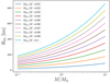 |
Fig. C.1 Rough estimation of the ocean depth at given ocean mass fraction according to Eq. (C.3). |
| In the text | |
Current usage metrics show cumulative count of Article Views (full-text article views including HTML views, PDF and ePub downloads, according to the available data) and Abstracts Views on Vision4Press platform.
Data correspond to usage on the plateform after 2015. The current usage metrics is available 48-96 hours after online publication and is updated daily on week days.
Initial download of the metrics may take a while.