| Issue |
A&A
Volume 646, February 2021
|
|
|---|---|---|
| Article Number | A178 | |
| Number of page(s) | 7 | |
| Section | Extragalactic astronomy | |
| DOI | https://doi.org/10.1051/0004-6361/202037888 | |
| Published online | 23 February 2021 | |
Detection of H2O and OH+ in z > 3 hot dust-obscured galaxies⋆
1
Department of Space, Earth and Environment, Chalmers University of Technology, Onsala Space Observatory, 439 92 Onsala, Sweden
e-mail: This email address is being protected from spambots. You need JavaScript enabled to view it.
2
CAS Key Laboratory for Research in Galaxies and Cosmology, Department of Astronomy, University of Science and Technology of China, Hefei 230026, PR China
3
School of Astronomy and Space Sciences, University of Science and Technology of China, Hefei, Anhui 230026, PR China
4
Joint ALMA Observatory (JAO) Alonso de Córdova 3107, Santiago, Chile
5
European Southern Observatory, Alonso de Córdova 3107, Casilla 19001, Vitacura, Santiago, Chile
Received:
5
March
2020
Accepted:
17
November
2020
Abstract
Aims. In this paper we present the detection of H2O and OH+ emission in z > 3 hot dust-obscured galaxies (Hot DOGs).
Methods. Using ALMA Band-6 observations of two Hot DOGs, we detected H2O(202 − 111) in W0149+2350, and H2O(312 − 303) and the multiplet OH+(11 − 01) in W0410−0913. These detections were serendipitous, falling within the side-bands of Band-6 observations aimed to study CO(9−8) in these Hot DOGs.
Results. We find that both sources have luminous H2O emission with line luminosities of LH2O(202 − 111) > 2.2 × 10⁸ L⊙ and LH2O(312 − 303) = 8.7 × 10⁸ L⊙ for W0149+2350 and W0410−0913, respectively. The H2O line profiles are similar to those seen for the neighbouring CO(9–8) line, with line widths of full width at half maximum (FWHM) ∼800−1000 km s−1. However, the H2O emission seems to be more compact than the CO(9−8). OH+(11 − 01) is detected in emission for W0410−0913, with a FWHM = 1000 km s−1 and a line luminosity of LOH+(11 − 01) = 6.92 × 10⁸ L⊙. The ratio of the observed H2O line luminosity over the IR luminosity, for both Hot DOGs, is consistent with previously observed star-forming galaxies and active galactic nuclei (AGN). The H2O/CO line ratio of both Hot DOGs and the OH+/H2O line ratio of W0410−0913 are comparable to those of luminous AGN found in the literature.
Conclusions. The bright H2O(202 − 111), and H2O(312 − 303) emission lines are likely due to the combined high star formation levels and luminous AGN in these sources. The presence of OH+ in emission, and the agreement of the observed line ratios of the Hot DOGs with luminous AGN in the literature, would suggest that the AGN emission is dominating the radiative output of these galaxies. However, follow-up multi-transition observations are needed to better constrain the properties of these systems.
Key words: galaxies: high-redshift / galaxies: ISM / galaxies: active / galaxies: evolution
The reduced spectra are only available at the CDS via anonymous ftp to cdsarc.u-strasbg.fr (130.79.128.5) or via http://cdsarc.u-strasbg.fr/viz-bin/cat/J/A+A/646/A178
© ESO 2021
1. Introduction
Energetic feedback from active galactic nuclei (AGN) has the potential to heat and remove the cold molecular gas from the interstellar medium (ISM), consequently suppressing the star formation of the host galaxy. The most successful models of galaxy formation and evolution require AGN feedback to explain many of the puzzling properties of local massive galaxies and the intergalactic medium (e.g., red colours, steep luminosity function, black-hole – spheroid relationship, and metal enrichment of the intergalactic medium; see Alexander & Hickox 2012, and Fabian 2012 for reviews). Understanding the properties of the molecular gas in the ISM of active galaxies is key to constraining and disentangling the effects of AGN and star formation.
Within the past few years the Wide-Infrared Survey Explorer (WISE; Wright et al. 2010) has led to the discovery of a population of luminous, dust-obscured AGN (e.g., Eisenhardt et al. 2012; Bridge et al. 2013; Lonsdale et al. 2015). Selected to be the reddest sources in the WISE colour-colour plot ([3.4–4.6] μm vs [4.6–12] μm), these galaxies are by definition highly obscured and dusty. They are commonly referred to as hot dust-obscured galaxies (Hot DOGs). This new class of galaxies is a rare sample with only 1000 over the entire sky (e.g., Eisenhardt et al. 2012). They are mostly high-redshift objects, at 1 < z < 4 (e.g., Wu et al. 2012; Tsai et al. 2015), and extremely luminous with Lbol > 1013 L⊙ (e.g., Jones et al. 2014; Wu et al. 2014). Based on X-ray observations and spectral energy distribution (SED) studies, there is clear evidence that they host highly dust-obscured AGN (e.g., Stern et al. 2014; Piconcelli et al. 2015; Assef et al. 2015, 2016; Fan et al. 2016a).
Hot DOGs are found in predominantly over-dense regions (e.g., Jones et al. 2017), and the most luminous among them show evidence of a high merger fraction (62% Fan et al. 2016b). This supports a scenario in which Hot DOGs could represent the post-merger transitional phase from a dusty starburst dominated phase to an optically bright quasar phase (e.g., Eisenhardt et al. 2012; Wu et al. 2012; Fan et al. 2016b). Their rarity could be a result of rare events such as major mergers, the relative briefness of the transitional phase they represent, and/or the population tracing the tail end of the mass function.
In this paper we present the detection of H2O, and OH+ emission lines for the first time in Hot DOGs. In the past few years there have been a number of detections of H2O transitions in the far-infrared (FIR) and submillimeter wavelengths with the advent of observatories such as Herschel, NOEMA, and ALMA. Studies of nearby galaxies have shown that H2O is the third most abundant species in dense, warm, star-forming regions, and shock heated regions (e.g., Cernicharo et al. 2006; Bergin et al. 2003; González-Alfonso et al. 2013). Detections of H2O transitions in high-z and lensed submillimeter galaxies confirm that they are among the strongest molecular lines in starburst galaxies and also show similar line profiles and spatial distribution as the high-J CO emission (e.g., Lis et al. 2011; van der Werf et al. 2011; Bradford et al. 2011; Combes et al. 2012; Lupu et al. 2012; Bothwell et al. 2013; Omont et al. 2013; Riechers et al. 2013; Weiß et al. 2013; Yang et al. 2016, 2019, 2020; Oteo et al. 2017; Apostolovski et al. 2019; Casey et al. 2019; Jarugula et al. 2019). Furthermore, there is a correlation between the line luminosity and the IR luminosity, extending over three orders of magnitude (e.g., Omont et al. 2013; Yang et al. 2013, 2016). Modelling of H2O emission in extragalactic sources has shown that the combination of different transitions can help disentangle the different components of the molecular ISM (e.g., González-Alfonso et al. 2014; Liu et al. 2017).
OH+ is an important part of the chemical network for the formation of H2O and can trace the ionisation rate of mixed atomic and molecular gas (e.g., Neufeld et al. 2010; Hollenbach et al. 2012), as well as the turbulent gas component (e.g., González-Alfonso et al. 2018). OH+ is observed both in emission and absorption in both low- and high-z galaxies (e.g., van der Werf et al. 2010; Spinoglio et al. 2012; Kamenetzky et al. 2012; Pereira-Santaella et al. 2013; Riechers et al. 2013; Gallerani et al. 2014; van der Tak et al. 2016; Li et al. 2020). Interestingly, OH+ is observed in emission for sources with a strong AGN component, (e.g., van der Werf et al. 2010; Spinoglio et al. 2012; Pereira-Santaella et al. 2013; Li et al. 2020), while starburst galaxies show OH+ in absorption (e.g., Kamenetzky et al. 2012; Riechers et al. 2013; van der Tak et al. 2016).
The two Hot DOGs discussed in this paper, W0149+2350 and W0410-0913, were selected to be among the most starbursting Hot DOGs, with massive molecular gas reservoirs discovered in CO(4−3) (Fan et al. 2018). Both sources have exceptionally wide CO lines in multiple transitions, with FWHM≈ 750−950 km s−1 (Fan et al. 2018; Knudsen et al., in prep.; see Table 1) and large molecular gas masses of 1010 − 1011 M⊙.
In Sect. 2 we present the ALMA observations and the extraction of the spectra. In Sect. 3 we present our results for the two sources, and in Sect. 4 we discuss the cause of excitation of the observed emission and compare this to the literature. Finally, in Sect. 5 we give the summary and conclusions. Throughout this paper we assume a WMAP7 cosmology.
2. ALMA observations and analysis
We obtained multi-band observations of W0149+2350 and W0410−0913 (project 2017.1.00123.S) to study CO rotational transitions, and these data yielded three serendipitous detections of other molecular lines. Observations were carried out using the Band-6 receivers, where one side-band was tuned to the redshifted CO(9–8) with the correlator used in frequency domain mode with each spectral window (spw) having a bandwidth of 1.875 GHz, the other sideband used a continuum set-up. Observations of W0149+2350 were carried out on 24 September 2018, with a total of 49 min of on-source integration time. The observed frequencies cover the ranges from 229.82 to 233.60 GHz and from 243.68 to 245.55 GHz, which include the redshifted H2O(202 − 111) transition in addition to the targeted CO(9–8). Observations of W0410−0913 were carried out on 7 September 2018, with a total of 6 min of on-source integration time. The observed frequencies cover the ranges from 221.08 to 224.81 GHz and from 236.28 to 240.57 GHz, which include the H2O(312 − 303) transition, and the OH+(11 − 01) multiplet in addition to the targeted CO(9–8). Flux and bandpass calibration was done using J0006−0623 and J0423−0120, and gain calibration was done with J0152+2207 and J0407−1211, for W0149+2350 and W0410−0913, respectively. Beam sizes correspond to 0.53″ × 0.32″ and 0.67″ × 0.52″ for W0149+2350 and W0410−0913, respectively.
Reduction, calibration, and imaging was done using CASA (Common Astronomy Software Application1; McMullin et al. 2007). The pipeline-reduced data delivered from the observatory were of sufficient quality; little or no additional flagging and further calibration were necessary. The steps required for standard reduction and calibration included in the pipeline include flagging, bandpass calibration, and flux and gain calibration. For our imaging process we applied natural weighting. A conservative estimate of the error on the absolute flux calibration is 10%. Continuum emission was subtracted using the line-free channels identified in both sidebands for each source. For both sources, the channel width was set to 60 km s−1.
To extract the spectrum we used the following procedure. We created the moment-0 map of each emission line, and used the IMFIT tool of CASA to get an estimate of the extent of the emission. We then extracted the spectrum from a region that is equivalent to two times the size estimate of the source.
In this paper we also show the CO(9−8) emission for comparison. This data has been extracted and analysed in the same way as the H2O and OH+ emission, which are the focus of this paper. However, the CO(9−8) data will be presented in more detail in Knudsen et al. (in prep.) along with other CO transitions.
3. Results
3.1. H2O(202 – 111) in W0149+2350
For W0149+2350 we detected H2O emission in the transition of H2O(202 − 111), see Table 2 and Fig. 1 (in yellow). Although the line is truncated, it covers ∼ 1000 km s−1 with a line profile that cannot be described by a single Gaussian. This type of line profile is also seen in their CO(9–8) line emission (see Fig. 1; Knudsen etal., in prep.).
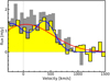 |
Fig. 1. Detected H2O line (yellow) of W0149+2350, with the CO(9−8) emission (grey) shown in the background for comparison. The fitted single and double Gaussians are shown with red and blue curves, respectively. |
Spectroscopic parameters of propynethial in MHz – S Reduction.
Identified lines based on the CDMS (https://cdms.astro.uni-koeln.de) catalogue entries and corresponding RMS of their spectrum (RMSspec).
In Fig. 1 we show the line with the fit of a single Gaussian and a double Gaussian. A double-Gaussian fit to the line improves the χ2 by 22% compared to the single-Gaussian fit. In Table 3 we give the fit results for the two-component fit to the line. However, as the line is truncated, we integrate the measured flux of the line to calculate a lower limit of the total integrated line flux (see Table 3).
Detected line properties.
In Fig. 2 we show the Hubble Space Telescope (HST) map from Fan et al. (2016b); the moment-0 map contours of the H2O emission are shown in blue and the CO contours are shown in yellow for comparison. To estimate the extent of the emission observed, we use the IMFIT tool of CASA, to fit to the moment-0 maps of each line. However, as the H2O line is truncated, to have a meaningful comparison of the extent of the emission we create moment-0 maps, limited to the velocity range of −300 < υ < 750 km s−1, for both the H2O and CO emission. We find that the H2O emission of W0149+2350 extends across 2.3 ± 0.6 kpc, while the CO(9−8) emission extends across 3.3 ± 0.5 kpc (see Table 4).
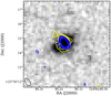 |
Fig. 2. HST WFC3 cut-out of W0149+2350. Overplotted are the contours corresponding to 3, 4, 5, 7, and 9σ for the H2O line (blue) and CO(9−8) line (yellow). The RMS values of the moment maps correspond to 0.046 Jy km s−1 and 0.055 Jy km s−1 for the H2O and CO(9−8) lines, respectively. Negative contours corresponding to −3σ are also plotted with dashed lines. |
Estimated size, based on a 2D fit to the moment-0 maps of each emission line.
3.2. H2O(312 – 303) and OH+(11 – 01) in W0410−0913
For W0410−0913 we detected the H2O(312 − 303) and OH+(11 − 01) multiplet with transitions at 1032.998–1033.118 GHz (see Table 2, although unresolved). Similar to what is seen for W0149+2350, the H2O(312 − 303) line also shows a very wide profile, which is similar to that of the CO(9−8).
In Fig. 3 we show the H2O(312 − 303) line, with the fit of a single Gaussian, and a double Gaussian. A double-Gaussian fit to the line improves the χ2 by 12% compared to the single-Gaussian fit. In Table 3 we give the results for the two-component fit to the line.
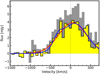 |
Fig. 3. Detected H2O line (yellow) of W0410−0913, with the CO(9−8) emission (grey) shown in the background for comparison. The fitted single and double Gaussians are shown with the red and blue curves, respectively. |
Owing to their large line widths, the CO(9−8) and OH+ lines are partially blended. We perform a simultaneous fit of the CO(9−8) and OH+ emission. We do this by using a double-Gaussian fit for the CO(9−8), and a single Gaussian for the OH+ emission. We allow all three parameters of the Gaussians to vary during the fit, restricting the central velocity (υcen) of each component of the CO line within a range of 400 km s−1, and for the OH+ line within 200 km s−1 of the expected υcen. In Fig. 5 we show the double-Gaussian fit to the CO(9−8) line and the resulting fit to the OH+ emission. In Table 3 we give line properties based on the fit. In this case the integrated line flux (Sint) is based on the fit. We note that in our analysis we assume that the OH+ is in emission based on the observed spectrum; however, it is possible that it has a different line profile, such as a P-Cygni profile, that is not visible owing to the blending with the CO(9−8) line. In some starburst galaxies OH+ has been found to have a P-Cygni line profile. An example is NGC253, for which it is concluded that the OH+ is primarily arising in cold diffuse foreground gas (van der Tak et al. 2016). If the OH+ multiplet observed here had a P-Cygni profile, it would require a strongly asymmetric line profile for the CO(9–8) to compensate for the superimposed absorption feature of the OH+. This would require luminous CO(9−8) emission at ∼1000 km s−1 from the line centre. Such a peculiar line profile is unlikely and is not seen for the lower-J CO (Fan et al. 2018; Knudsen et al., in prep.) and H2O transitions. It could also be possible for the emission identified as OH+ to be alternatively interpreted as a massive and highly excited molecular outflow. However, such a scenario would require a combination of orientation and foreground absorption that would allow us to see the red component of the outflow, while not seeing emission from the blue component. Furthermore, there is no evidence for such a massive outflow in the lower-J CO transitions (Fan et al. 2018; Knudsen et al., in prep.).
In Fig. 4 we show the HST map from Fan et al. (2016b), with the moment-0 map contours of the H2O emission in blue, the OH+ emission in white, and the CO contours in yellow for comparison. The OH+ emission closely follows the extent seen in the CO(9−8), which shows an extended non-uniform structure, but the H2O emission is more compact. We estimate the extent of the emission observed using the IMFIT tool of CASA. Following the analysis of W0149+2350, we create moment-0 maps limited to the velocity range of −500 < υ < 500 km s−1, for the H2O, CO, and OH+ emission, to match to the velocity range covered by the H2O line. The OH+ is extended across 9.3 ± 2.1 kpc, similar to the CO(9−8) emission extending over 5.7 ± 0.6 kpc, while the H2O is more compact covering 3.0 ± 0.6 kpc. The extent of the CO(9−8) and OH+ emission is significantly larger than the H2O; however, deeper and higher resolution observations are needed to better constrain these properties and to further interpret these results.
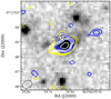 |
Fig. 4. HST WFC3 cut-out of W0410-0913. Overplotted are the contours corresponding to 3, 4, 5, 7, and 9σ, for the H2O line (blue), OH+ line (white), and CO(9−8) line (yellow). The RMS values of the moment maps correspond to 0.12 Jy km s−1, 0.146 Jy km s−1, and 0.116 Jy km s−1 for the H2O, OH+ and CO(9−8) lines, respectively. Negative contours corresponding to −3σ are also plotted with dashed lines. |
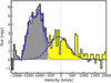 |
Fig. 5. Detected OH+ line (yellow) of W0410−0913, next to the CO(9−8) line (grey). The grey colour also shows the channels used to fit the CO(9−8) line. The dotted blue curve shows the double-Gaussian fit to the CO(9−8), the dashed blue curve shows the single-Gaussian fit to the OH+ emission, and the solid curve is the combination of the above. |
For both sources we find that the high-density gas traced by H2O extends over scales of a few kiloparsec. Based on the total gas masses estimated by Fan et al. (2018), and if we assume a spherical geometry2 with radii of 1–2 kpc and a volume filling factor of 0.01–0.1%, then the estimated gas density is in the range n(H2) ∼ 105 − 106 cm−3. This agrees with what is required for the excitation of the observed H2O emission. Therefore, the extent of the observed emission is consistent with the gas mass estimated for these galaxies.
4. Discussion
4.1. Excitation of the H2O and OH+ emission
In a detailed study of H2O submillimetre lines in the nuclei of nearby star-forming galaxies, Liu et al. (2017) used modelling to determine the physical conditions and excitation mechanisms needed for the H2O transitions of low, medium, and high energy levels. Liu et al. (2017) examined three components of the molecular ISM: a cold component with densities of n(H2) ∼ 104 − 106 cm−3, dust temperatures of Td ∼ 20−30 K, and column densities of N((H2) ∼ 1023 cm−2; a warm component with n((H2) ∼ 105 − 106 cm−3, Td ∼ 40−70 K, and N(H2) ∼ 1−4 × 1024 cm−2; and a hot component with n((H2) ≥ 106 cm−3, Td ∼ 100−200 K, N(H2) ≥ 5 × 1024 cm−2. Interestingly, the H2O(202 − 111) transition can trace both the warm and hot components, but the H2O(312 − 303) transition is stronger in the warm component of the ISM and is not strongly produced in hot ISM conditions. Based on the radiative-transfer analysis of Liu et al. (2017) the H2O(202 − 111) and H2O(312 − 303), transitions can be produced by collisional excitation alone, while higher-energy transitions characteristic of the hot ISM component require IR pumping to reach the observed intensities. However, González-Alfonso et al. (2014), which also modelled the H2O submillimetre lines for IR galaxies, argued that IR pumping has a significant role in producing the H2O(202 − 111) and H2O(312 − 303) line emission. In both cases, higher-energy transitions are more likely to exclusively trace the hot component of the ISM surrounding AGN. Indeed, there was recently a detection of H2O(414 − 321) from the circumnuclear disc of a lensed quasar (Stacey et al. 2020).
As we only have a single H2O line detection for each source, it is not possible to make an extensive analysis. But we take a simplistic modelling approach using the non-local thermodynamic equilibrium (non-LTE) molecular radiative transfer code RADEX (van der Tak et al. 2007) to provide some constraints on the possible excitation of the observed H2O emission.
We use the peak fluxes for each of the observed H2O lines and the corresponding CO(9−8) line for each source. We assume a spherical symmetry and CO column densities in the range of 1016 − 1017 cm−2 to avoid optically thin emission at the low end and opacities that are too high at the high end. Based on the SED fit and decomposition of these sources (Tsai et al. 2015; Fan et al. 2016a), we expect an AGN torus dust temperature of 450 K and a dust temperature due to star formation of 51 K and 63 K.
For W0149+2350, we find that the H2O(202 − 111) transition, at 987.94 GHz (EL = 53 K), may be collisionally excited. For intermediate densities (≤106 cm−3), relatively high H2O(202 − 111) abundances (> 10−6) are required. At higher densities (> 106 cm−3), lower abundances of 10−7 − 10−8 are possible. For W0410−0913, we find that the H2O(312 − 303) transition, at 1097.36 GHz (EL = 196 K) line may be collisionally excited, but that would require densities > 106 cm−3. Even for these high densities, the H2O(312 − 303) abundance is rather high (10−5 − 10−6). However, for both sources, it is unlikely to have such high densities filling the region corresponding to the beam at these distances (i.e. ∼4–5 kpc). This can either be solved with a small filling factor of dense clumps and/or the emission emerging from a dense nuclear structure (e.g., the AGN torus). Alternatively, all or parts of the H2O emission are being influenced by IR pumping, which would allow this emission to arise also in lower-density gas. This agrees with what is argued in González-Alfonso et al. (2014).
Based on the results of our simplistic RADEX modelling and what has been found by González-Alfonso et al. (2014) and Liu et al. (2017), we expect that the transitions that we detected are due to the high levels of star formation in our sources; there is a possibly significant contribution from the AGN (through IR pumping).
So far in the literature, sources where the OH+ line is in emission have been galaxies with significant AGN contributions such as Mrk231 (van der Werf et al. 2010), NGC1068 (Spinoglio et al. 2012), and NGC7130 (Pereira-Santaella et al. 2013). Therefore, the detection of OH+ in emission for W0410−0913 could be indicative of excitation from cosmic rays and X-rays from the AGN (e.g., van der Werf et al. 2010; Spinoglio et al. 2012; Pereira-Santaella et al. 2013; Li et al. 2020). The relative line intensities between the CO(9−8), the OH+(11 − 01) multiplet, and the H2O(312 − 303) observed for W0410−0913 are consistent with those of Mrk231 (van der Werf et al. 2010), for which it was shown that the combination of strong high-J CO, and OH+ emission indicate X-ray driven excitation from the AGN of Mrk231. However, owing to the limitations of our data and the lack of other HnO+ transitions, we cannot confirm that the OH+ emission is due to the AGN through radiative transfer modelling.
4.2. H2O–IR luminosity ratio of Hot DOGs
The relationship between the H2O line luminosity with IR luminosity (from 8 to 1000 μm; LIR), and the ratio of the two, has been closly studied for low- and high-z, dusty, star-forming galaxies (see e.g., Yang et al. 2013, 2016; Jarugula et al. 2019). In this section, we compare the two detected Hot-DOGs of this paper to low- and high-z ultra-luminous IR galaxies (ULIRGs), submillimetre galaxies (SMGs), and AGN in the literature. We only compare to sources with the same H2O transition available as each of the sources.
As our sources have both a strong AGN and star formation contribution to the total LIR, it is important to consider how we compare the H2O line luminosity and the IR luminosity. For example, if the observed H2O emission is primarily tracing the star formation in our source, then we should take the ratio with the IR luminosity due to star formation (LIR, SF); however, if the emission is tracing both AGN and star formation regions, then the total IR luminosity should be considered (LIR, tot). It is not possible in our analysis to confidently distinguish if the H2O emission is only due to the star formation of the source, as excitation from the AGN could also be contributing significantly. For this reason we examine both of the possible scenarios when comparing to the literature.
In the top panel of Fig. 6 we show the ratio of the line luminosity for the H2O(202 − 111) transition over LIR (LH2O(202 − 111)/LIR) as a function of LIR. We plot two values for W0149+2350, LH2O(202 − 111)/LIR, tot > 0.25 × 10⁻⁵ and LH2O(202 − 111)/LIR, SF > 2 × 10⁻⁵, in comparison to both strong AGN and ULIRGs/SMGs that have been detected in the same transition. As we only have a lower limit for W0149+2350 the LH2O(202 − 111)/LIR, tot ratio, although low, is consistent with both AGN and ULIRGs/SMGs at low- and high-z. However, the lower limit for LH2O(202 − 111)/LIR, SF, is only consistent with luminous high-z ULIRGs/SMGs, as can be expected if the source of the H2O emission are the star formation regions.
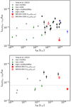 |
Fig. 6. Ratio of the H2O line luminosity over the IR luminosity (LH2O/LIR), as a function of LIR, for the two Hot DOGs. Top: W0149+2350 in comparison to literature sources with detected H2O(202−111) emission, labelled based on their classification (van der Werf et al. 2011; Combes et al. 2012; Bothwell et al. 2013; Omont et al. 2013; Riechers et al. 2013; Falstad et al. 2015, 2017; Yang et al. 2016; Liu et al. 2017; Oteo et al. 2017; Apostolovski et al. 2019; Jarugula et al. 2019). Also shown are the average ratios found by Yang et al. (2013) for nearby IR galaxies. Bottom: W0410−0913 in comparison to literature sources with detected H2O(312−303) emission, labelled based on their classification (Riechers et al. 2013; Falstad et al. 2015, 2017; Liu et al. 2017; Oteo et al. 2017); the average ratios found by Yang et al. (2013) for nearby IR galaxies are also shown. |
In the bottom panel of Fig. 6 we show the ratio for the H2O(312−303) transition (LH2O(312 − 303)/LIR) as a function of LIR. Again, we plot two values corresponding to W0410−0913, LH2O(312 − 303)/LIR, tot = 0.44 × 10⁻⁵ and LH2O(312 − 303)/LIR, SF = 1.86 × 10⁻⁵. In this case, the LH2O(312 − 303)/LIR, tot ratio of W0410−0913 is consistent with low-z AGN and ULIRGs, but is significantly below what is seen for high-z ULIRGs/SMGs, while the LH2O(312 − 303)/LIR, SF ratio is consistent with the high-z ULIRGs/SMGs.
4.3. H2O and OH+ line ratios of Hot DOGs
In this section we compare the observed H2O and OH+ line ratios of our sources to the ratios in other galaxies found in the literature. We find that for W0149+2350 the H2O(202 − 111)/CO(9−8) ratio is > 0.5. This is in agreement with what is seen in the literature for high–z ULIRGs/SMGs and AGN (0.5–0.8 for ULIRGs/SMGs, and 0.4–0.7 for AGN; e.g., Apostolovski et al. 2019; Bradford et al. 2009; Jarugula et al. 2019; Li et al. 2020; Oteo et al. 2017; Riechers et al. 2013; van der Werf et al. 2011; Weiß et al. 2007). However, the ratio of H2O(202−111)/CO(4−3) is > 1.4, which is significantly higher than what has been observed for high–z ULIRGs/SMGs (0.4–0.85; e.g., Bradford et al. 2009; Jarugula et al. 2019; Omont et al. 2013; Yang et al. 2016, 2017), although consistent with the luminous AGN APM08279+5255 that has H2O(202−111)/CO(4−3) value of 2.4 (van der Werf et al. 2011; Weiß et al. 2007).
For W0410−0913, we calculate line ratios of H2O(312−303)/CO(9−8) = 0.8 ± 0.2, H2O(312−303)/CO(4−3) = 0.6 ± 0.1 and OH+(11−01)/H2O(312−303) = 0.8 ± 0.2. In this case, there are a limited number of similar measurements available in the literature. However, the H2O(312−303)/CO(9−8) ratio of W0410−0913 is consistent if somewhat higher than high–z ULIRGs/SMGs (0.4–0.75; e.g., Oteo et al. 2017; Riechers et al. 2013). The OH+(11−01)/H2O(312−303) ratio is consistent with low–z luminous AGN (e.g., Mrk231 and NGC1068; van der Werf et al. 2010; Liu et al. 2017; Spinoglio et al. 2012).
The nearby ULIRG Mrk231 is particularly interesting to compare to as it has a luminous AGN that contributes 70% of the IR luminosity, similar to that found for our Hot DOGs with 87% and 77% in W0149+2350 and W0410−0913, respectively (Fan et al. 2016a). Mrk231 has H2O(202−111)/CO(4−3) and H2O(312−303)/CO(4−3) line ratios of 0.4 (e.g., van der Werf et al. 2010; Papadopoulos et al. 2007), and an OH+(11−01)/H2O(312−303) ratio of 0.65 (van der Werf et al. 2010; Liu et al. 2017). Overall, W0410−0913 seems most consistent with that seen for Mrk231, while for W0149+2350 the H2O(202−111)/CO(4−3) ratio is significantly larger than for Mrk231. Interestingly, W0149+2350 also has a significantly larger AGN contribution to the IR luminosity than W0410−0913 and Mrk231.
5. Summary and conclusions
In this paper we have presented the recent detection of H2O and OH+ in z > 3 Hot DOGs. This is the first detection of these emission lines for this class of galaxies, and one of the few in high-z non-lensed galaxies (e.g., Casey et al. 2019). Specifically, we detected the H2O(202−111) transition from W0149+2350, and the H2O(312−303), and the OH+(11 − 01) multiplet from W0410−0913. These were serendipitous detections in an observation programme targeting the CO(9−8) emission of these sources (Knudsen et al., in prep.).
Similar to that found for previously observed high-z ULIRGs and SMGs, the line profile of the H2O emission lines follows that of the high-J CO(9−8) emission. But the extent of the H2O emission seems to be more compact than that of CO(9−8), and in the case of W0410−0913 it is more compact than the OH+(11 − 01) emission too. However, deeper and higher resolution observations are needed to better constrain the emission properties and to further interpret these results.
A single H2O line detection does not allow us to disentangle the ISM components and determine the molecular gas properties. However, the luminous H2O emission in these two Hot DOGs indicate the existence of warm dense molecular gas conditions (n(H2) ∼ 105 − 106 cm−3, Td ∼ 40−70 K), possibly dominated by collisional excitation, and has a likely contribution from IR pumping from the AGN. We cannot confidently distinguish between excitation due to the AGN, star formation, or both for the H2O emission. However, the detection of OH+(11 − 01) in emission for W0410−0913, and the agreement of the observed line ratios with luminous AGN in the literature, indicate that the energy output from the AGN is dominating the radiative output of this galaxy, even though there is significant ongoing star formation (1000–5000 M⊙ yr−1). This is consistent with the fact that these galaxies host AGN that dominate the IR luminosity, contributing ≳70% (Fan et al. 2016a). This would also be consistent with the scenario that Hot DOGs are going through a transitional phase from a starburst–dominated to an AGN–dominated phase (e.g., Eisenhardt et al. 2012; Wu et al. 2012; Fan et al. 2016b).
In order to break the degeneracies and disentangle the relative contributions from the AGN and the star formation, a multi-transitional approach is required. Based on the results of modelling studies (e.g., González-Alfonso et al. 2014; Liu et al. 2017), it is possible to design observational programmes targeting a combination of H2O transitions that trace different components of the molecular gas. Transitions such as H2O(202−111) and H2O(312−303), which have energies of Eup < 250 − 350 K, can be produced by collisional excitation alone or a combination of collisional excitation and IR pumping. However, higher energy transitions, such as H2O(414 − 321) or H2O(422−413), require IR pumping and are therefore more likely to directly trace excitation from the AGN. A combination of H2O transitions from low, medium, and high energy levels, could be a useful tool for disentangling the AGN and star formation contributions to the excitation of the dense molecular gas. Furthermore, targeting additional HnO+ transitions, such as H2O+ and H3O+ in combination with OH+, would allow for constraints on the chemistry and excitation of the diffuse gas of these galaxies, possibly directly connected to the AGN (see e.g., González-Alfonso et al. 2013, 2018, for detailed analysis).
We note that if we instead assume a cylindrical geometry with a radius based on the estimated sizes from Table 4 and a height of 0.5 kpc, our results remain the same.
Acknowledgments
We thank the anonymous referee for constructive comments. We thank the staff of the Nordic ALMA Regional Center node for their support and helpful discussions. We thank Dr Hannah Calcutt and Dr. Pierre Cox for helpful discussions. K.K. acknowledges support from the Knut and Alice Wallenberg Foundation. S.A. acknowledges support from the European Research Council (ERC) and the Swedish Research Council. L.F. acknowledges the support from the National Natural Science Foundation of China (NSFC Nos. 11822303, 11773020 and 11421303) and Shandong Provincial Natural Science Foundation (JQ201801). This paper makes use of the following ALMA data: ADS/JAO.ALMA#2017.1.00123.S. ALMA is a partnership of ESO (representing its member states), NSF (USA) and NINS (Japan), together with NRC (Canada) and NSC and ASIAA (Taiwan) and KASI (Republic of Korea), in cooperation with the Republic of Chile. The Joint ALMA Observatory is operated by ESO, AUI/NRAO and NAOJ.
References
- Alexander, D. M., & Hickox, R. C. 2012, New Astron. Rev., 56, 93 [NASA ADS] [CrossRef] [Google Scholar]
- Apostolovski, Y., Aravena, M., Anguita, T., et al. 2019, A&A, 628, A23 [NASA ADS] [CrossRef] [EDP Sciences] [Google Scholar]
- Assef, R. J., Eisenhardt, P. R. M., Stern, D., et al. 2015, ApJ, 804, 27 [NASA ADS] [CrossRef] [Google Scholar]
- Assef, R. J., Walton, D. J., Brightman, M., et al. 2016, ApJ, 819, 111 [NASA ADS] [CrossRef] [Google Scholar]
- Bergin, E. A., Kaufman, M. J., Melnick, G. J., Snell, R. L., & Howe, J. E. 2003, ApJ, 582, 830 [NASA ADS] [CrossRef] [Google Scholar]
- Bothwell, M. S., Aguirre, J. E., Chapman, S. C., et al. 2013, ApJ, 779, 67 [Google Scholar]
- Bradford, C. M., Aguirre, J. E., Aikin, R., et al. 2009, ApJ, 705, 112 [NASA ADS] [CrossRef] [Google Scholar]
- Bradford, C. M., Bolatto, A. D., Maloney, P. R., et al. 2011, ApJ, 741, L37 [NASA ADS] [CrossRef] [Google Scholar]
- Bridge, C. R., Blain, A., Borys, C. J. K., et al. 2013, ApJ, 769, 91 [NASA ADS] [CrossRef] [Google Scholar]
- Casey, C. M., Zavala, J. A., Aravena, M., et al. 2019, ApJ, 887, 55 [Google Scholar]
- Cernicharo, J., Goicoechea, J. R., Daniel, F., et al. 2006, ApJ, 649, L33 [Google Scholar]
- Combes, F., Rex, M., Rawle, T. D., et al. 2012, A&A, 538, L4 [NASA ADS] [CrossRef] [EDP Sciences] [Google Scholar]
- Eisenhardt, P. R. M., Wu, J., Tsai, C.-W., et al. 2012, ApJ, 755, 173 [NASA ADS] [CrossRef] [EDP Sciences] [Google Scholar]
- Fabian, A. C. 2012, ARA&A, 50, 455 [Google Scholar]
- Falstad, N., González-Alfonso, E., Aalto, S., et al. 2015, A&A, 580, A52 [NASA ADS] [CrossRef] [EDP Sciences] [Google Scholar]
- Falstad, N., González-Alfonso, E., Aalto, S., & Fischer, J. 2017, A&A, 597, A105 [NASA ADS] [CrossRef] [EDP Sciences] [Google Scholar]
- Fan, L., Han, Y., Fang, G., et al. 2016a, ApJ, 822, L32 [NASA ADS] [CrossRef] [Google Scholar]
- Fan, L., Han, Y., Nikutta, R., Drouart, G., & Knudsen, K. K. 2016b, ApJ, 823, 107 [Google Scholar]
- Fan, L., Knudsen, K. K., Fogasy, J., & Drouart, G. 2018, ApJ, 856, L5 [NASA ADS] [CrossRef] [Google Scholar]
- Gallerani, S., Ferrara, A., Neri, R., & Maiolino, R. 2014, MNRAS, 445, 2848 [Google Scholar]
- González-Alfonso, E., Fischer, J., Bruderer, S., et al. 2013, A&A, 550, A25 [NASA ADS] [CrossRef] [EDP Sciences] [Google Scholar]
- González-Alfonso, E., Fischer, J., Aalto, S., & Falstad, N. 2014, A&A, 567, A91 [NASA ADS] [CrossRef] [EDP Sciences] [Google Scholar]
- González-Alfonso, E., Fischer, J., Bruderer, S., et al. 2018, ApJ, 857, 66 [NASA ADS] [CrossRef] [Google Scholar]
- Hollenbach, D., Kaufman, M. J., Neufeld, D., Wolfire, M., & Goicoechea, J. R. 2012, ApJ, 754, 105 [NASA ADS] [CrossRef] [Google Scholar]
- Jarugula, S., Vieira, J. D., Spilker, J. S., et al. 2019, ApJ, 880, 92 [Google Scholar]
- Jones, S. F., Blain, A. W., Stern, D., et al. 2014, MNRAS, 443, 146 [NASA ADS] [CrossRef] [Google Scholar]
- Jones, S. F., Blain, A. W., Assef, R. J., et al. 2017, MNRAS, 469, 4565 [NASA ADS] [CrossRef] [Google Scholar]
- Kamenetzky, J., Glenn, J., Rangwala, N., et al. 2012, ApJ, 753, 70 [Google Scholar]
- Li, J., Wang, R., Riechers, D., et al. 2020, ApJ, 889, 162 [CrossRef] [Google Scholar]
- Lis, D. C., Neufeld, D. A., Phillips, T. G., Gerin, M., & Neri, R. 2011, ApJ, 738, L6 [NASA ADS] [CrossRef] [Google Scholar]
- Liu, L., Weiß, A., Perez-Beaupuits, J. P., et al. 2017, ApJ, 846, 5 [NASA ADS] [CrossRef] [Google Scholar]
- Lonsdale, C. J., Lacy, M., Kimball, A. E., et al. 2015, ApJ, 813, 45 [NASA ADS] [CrossRef] [Google Scholar]
- Lupu, R. E., Scott, K. S., Aguirre, J. E., et al. 2012, ApJ, 757, 135 [NASA ADS] [CrossRef] [Google Scholar]
- McMullin, J. P., Waters, B., Schiebel, D., Young, W., & Golap, K. 2007, in CASA Architecture and Applications, eds. R. A. Shaw, F. Hill, & D. J. Bell, ASP Conf. Ser., 376, 127 [Google Scholar]
- Neufeld, D. A., Goicoechea, J. R., Sonnentrucker, P., et al. 2010, A&A, 521, L10 [NASA ADS] [CrossRef] [EDP Sciences] [Google Scholar]
- Omont, A., Yang, C., Cox, P., et al. 2013, A&A, 551, A115 [NASA ADS] [CrossRef] [EDP Sciences] [Google Scholar]
- Oteo, I., Zwaan, M. A., Ivison, R. J., Smail, I., & Biggs, A. D. 2017, ApJ, 837, 182 [NASA ADS] [CrossRef] [Google Scholar]
- Papadopoulos, P. P., Isaak, K. G., & van der Werf, P. P. 2007, ApJ, 668, 815 [NASA ADS] [CrossRef] [Google Scholar]
- Pereira-Santaella, M., Spinoglio, L., Busquet, G., et al. 2013, ApJ, 768, 55 [NASA ADS] [CrossRef] [Google Scholar]
- Piconcelli, E., Vignali, C., Bianchi, S., et al. 2015, A&A, 574, L9 [NASA ADS] [CrossRef] [EDP Sciences] [Google Scholar]
- Riechers, D. A., Bradford, C. M., Clements, D. L., et al. 2013, Nature, 496, 329 [Google Scholar]
- Spinoglio, L., Pereira-Santaella, M., Busquet, G., et al. 2012, ApJ, 758, 108 [NASA ADS] [CrossRef] [Google Scholar]
- Stacey, H. R., Lafontaine, A., & McKean, J. P. 2020, MNRAS, 493, 5290 [Google Scholar]
- Stern, D., Lansbury, G. B., Assef, R. J., et al. 2014, ApJ, 794, 102 [NASA ADS] [CrossRef] [Google Scholar]
- Tsai, C.-W., Eisenhardt, P. R. M., Wu, J., et al. 2015, ApJ, 805, 90 [NASA ADS] [CrossRef] [Google Scholar]
- van der Tak, F. F. S., Black, J. H., Schöier, F. L., Jansen, D. J., & van Dishoeck, E. F. 2007, A&A, 468, 627 [NASA ADS] [CrossRef] [EDP Sciences] [Google Scholar]
- van der Tak, F. F. S., Weiß, A., Liu, L., & Güsten, R. 2016, A&A, 593, A43 [NASA ADS] [CrossRef] [EDP Sciences] [Google Scholar]
- van der Werf, P. P., Isaak, K. G., Meijerink, R., et al. 2010, A&A, 518, L42 [NASA ADS] [CrossRef] [EDP Sciences] [Google Scholar]
- van der Werf, P. P., Berciano Alba, A., Spaans, M., et al. 2011, ApJ, 741, L38 [NASA ADS] [CrossRef] [Google Scholar]
- Weiß, A., Downes, D., Neri, R., et al. 2007, A&A, 467, 955 [NASA ADS] [CrossRef] [EDP Sciences] [Google Scholar]
- Weiß, A., De Breuck, C., Marrone, D. P., et al. 2013, ApJ, 767, 88 [NASA ADS] [CrossRef] [Google Scholar]
- Wright, E. L., Eisenhardt, P. R. M., Mainzer, A. K., et al. 2010, AJ, 140, 1868 [Google Scholar]
- Wu, J., Tsai, C.-W., Sayers, J., et al. 2012, ApJ, 756, 96 [NASA ADS] [CrossRef] [Google Scholar]
- Wu, J., Bussmann, R. S., Tsai, C.-W., et al. 2014, ApJ, 793, 8 [NASA ADS] [CrossRef] [Google Scholar]
- Yang, C., Gao, Y., Omont, A., et al. 2013, ApJ, 771, L24 [NASA ADS] [CrossRef] [Google Scholar]
- Yang, C., Omont, A., Beelen, A., et al. 2016, A&A, 595, A80 [NASA ADS] [CrossRef] [EDP Sciences] [Google Scholar]
- Yang, C., Omont, A., Beelen, A., et al. 2017, A&A, 608, A144 [NASA ADS] [CrossRef] [EDP Sciences] [Google Scholar]
- Yang, C., Gavazzi, R., Beelen, A., et al. 2019, A&A, 624, A138 [NASA ADS] [CrossRef] [EDP Sciences] [Google Scholar]
- Yang, C., González-Alfonso, E., Omont, A., et al. 2020, A&A, 634, L3 [CrossRef] [EDP Sciences] [Google Scholar]
All Tables
Identified lines based on the CDMS (https://cdms.astro.uni-koeln.de) catalogue entries and corresponding RMS of their spectrum (RMSspec).
All Figures
|
Fig. 1. Detected H2O line (yellow) of W0149+2350, with the CO(9−8) emission (grey) shown in the background for comparison. The fitted single and double Gaussians are shown with red and blue curves, respectively. |
| In the text | |
|
Fig. 2. HST WFC3 cut-out of W0149+2350. Overplotted are the contours corresponding to 3, 4, 5, 7, and 9σ for the H2O line (blue) and CO(9−8) line (yellow). The RMS values of the moment maps correspond to 0.046 Jy km s−1 and 0.055 Jy km s−1 for the H2O and CO(9−8) lines, respectively. Negative contours corresponding to −3σ are also plotted with dashed lines. |
| In the text | |
|
Fig. 3. Detected H2O line (yellow) of W0410−0913, with the CO(9−8) emission (grey) shown in the background for comparison. The fitted single and double Gaussians are shown with the red and blue curves, respectively. |
| In the text | |
|
Fig. 4. HST WFC3 cut-out of W0410-0913. Overplotted are the contours corresponding to 3, 4, 5, 7, and 9σ, for the H2O line (blue), OH+ line (white), and CO(9−8) line (yellow). The RMS values of the moment maps correspond to 0.12 Jy km s−1, 0.146 Jy km s−1, and 0.116 Jy km s−1 for the H2O, OH+ and CO(9−8) lines, respectively. Negative contours corresponding to −3σ are also plotted with dashed lines. |
| In the text | |
|
Fig. 5. Detected OH+ line (yellow) of W0410−0913, next to the CO(9−8) line (grey). The grey colour also shows the channels used to fit the CO(9−8) line. The dotted blue curve shows the double-Gaussian fit to the CO(9−8), the dashed blue curve shows the single-Gaussian fit to the OH+ emission, and the solid curve is the combination of the above. |
| In the text | |
|
Fig. 6. Ratio of the H2O line luminosity over the IR luminosity (LH2O/LIR), as a function of LIR, for the two Hot DOGs. Top: W0149+2350 in comparison to literature sources with detected H2O(202−111) emission, labelled based on their classification (van der Werf et al. 2011; Combes et al. 2012; Bothwell et al. 2013; Omont et al. 2013; Riechers et al. 2013; Falstad et al. 2015, 2017; Yang et al. 2016; Liu et al. 2017; Oteo et al. 2017; Apostolovski et al. 2019; Jarugula et al. 2019). Also shown are the average ratios found by Yang et al. (2013) for nearby IR galaxies. Bottom: W0410−0913 in comparison to literature sources with detected H2O(312−303) emission, labelled based on their classification (Riechers et al. 2013; Falstad et al. 2015, 2017; Liu et al. 2017; Oteo et al. 2017); the average ratios found by Yang et al. (2013) for nearby IR galaxies are also shown. |
| In the text | |
Current usage metrics show cumulative count of Article Views (full-text article views including HTML views, PDF and ePub downloads, according to the available data) and Abstracts Views on Vision4Press platform.
Data correspond to usage on the plateform after 2015. The current usage metrics is available 48-96 hours after online publication and is updated daily on week days.
Initial download of the metrics may take a while.