| Issue |
A&A
Volume 645, January 2021
|
|
|---|---|---|
| Article Number | A39 | |
| Number of page(s) | 8 | |
| Section | Astrophysical processes | |
| DOI | https://doi.org/10.1051/0004-6361/202038826 | |
| Published online | 05 January 2021 | |
Magnetic deformation of neutron stars in scalar-tensor theories
1
Dipartimento di Fisica e Astronomia, Università degli Studi di Firenze, Via G. Sansone 1, 50019 Sesto F. no (Firenze), Italy
2
INAF – Osservatorio Astrofisico di Arcetri, Largo E. Fermi 5, 50125 Firenze, Italy
e-mail: This email address is being protected from spambots. You need JavaScript enabled to view it.
3
INFN – Sezione di Firenze, Via G. Sansone 1, 50019 Sesto F. no (Firenze), Italy
Received:
2
July
2020
Accepted:
27
October
2020
Abstract
Scalar-tensor theories are among the most promising alternatives to general relativity that have been developed to account for some long-standing issues in our understanding of gravity. Some of these theories predict the existence of a non-linear phenomenon that is spontaneous scalarisation, which can lead to the appearance of sizable modifications to general relativity in the presence of compact matter distributions, namely neutron stars. On the one hand, one of the effects of the scalar field is to modify the emission of gravitational waves that are due to both variations in the quadrupolar deformation of the star and the presence of additional modes of emission. On the other hand, neutron stars are known to harbour extremely powerful magnetic fields which can affect their structure and shape, leading, in turn, to the emission of gravitational waves – in this case due to a magnetic quadrupolar deformation. In this work, we investigate how the presence of spontaneous scalarisation can affect the magnetic deformation of neutron stars and their emission of quadrupolar gravitational waves, both of tensor and scalar nature. We show that it is possible to provide simple parametrisations of the magnetic deformation and gravitational wave power of neutron stars in terms of their baryonic mass, circumferential radius, and scalar charge, while also demonstrating that a universal scaling exists independently of the magnetic field geometry and of the parameters of the scalar-tensor theory. Finally, we comment on the observability of the deviations in the strain of gravitational waves from general relativity by current and future observatories.
Key words: gravitation / stars: magnetic field / stars: neutron / gravitational waves / magnetohydrodynamics (MHD) / relativistic processes
© ESO 2021
1. Introduction
Scalar-tensor theories (STTs) are among the most studied alternatives to general relativity (GR). Since the pioneering paper by Brans & Dicke (1961), much work has been devoted to study STTs and their phenomenology (Matsuda & Nariai 1973; Novak 1998; Fujii & Maeda 2003; Zhang et al. 2019). The main premise is taking a scalar field, which is non-minimally coupled to the metric and which plays the role of an effective space-time dependent gravitational “constant”, and adding it to the gravitational action. The effects of the scalar field manifest themselves in the presence of matter, which acts as a source for the scalar field. They range from cosmological scales, where the non-minimal coupling can account for cosmological observations without needing to resort to the existence of a dark sector (see e.g. Capozziello & de Laurentis 2011), up to the small scales of compact objects. Unfortunately, black holes are not useful in constraining STTs because the no-hair theorem also holds in such theories, preventing them from developing a scalar charge (Hawking 1972; Berti et al. 2015). This means that neutron stars (NSs) hold a special importance in testing GR – and even more so given that their compactness allows the scalar field to manifest its effects in a non-perturbative fashion through spontaneous scalarisation (Damour & Esposito-Farèse 1993), while allowing the tight observational constraints in the weak-gravity regime to be fullfilled (Shao et al. 2017). These effects are of a varied nature, including the emission of additional modes of gravitational waves (GWs; Pang et al. 2020), a modified relation between the NS mass and radius and its central density, a modification of NS merger dynamics (Shibata et al. 2014), as well as a variation in the frequency of normal modes of NSs (Sotani & Kokkotas 2005) in their tidal and rotational deformation (Pani & Berti 2014; Doneva et al. 2014) and their light propagation (Bucciantini & Soldateschi 2020).
There are various effects that can induce quadrupolar modifications in the shape of NSs. For example, crustal deformations could lead to the formation of mountains on the surface of the NS (Haskell et al. 2006), which would then cause the emission of continuous GWs (CGWs; Ushomirsky et al. 2000). Mountains are also expected to form during accretion in a process called magnetic burial (Melatos & Payne 2005). GWs are expected to be also released during starquakes, following a rearrangement of the magnetic field of the star, which may excite some of its oscillation modes (Keer & Jones 2015). Moreover, oscillation modes such as the axial r-mode are unstable due to the emission of GWs (Andersson 1998). Finally, if the magnetic axis of a NS is not aligned to its rotation axis, the star acquires a time-varying quadrupolar deformation which leads to the emission of CGWs, and it is believed that a NS endowed with a strong toroidal magnetic field will develop an instability which flips the star to an orthogonal rotator, maximising its emission of CGWs (Cutler 2002). This is particularly relevant in the context of newly born and rapidly rotating magnetars, which have been invoked as possible engines for long and short gamma-ray bursts (Dall’Osso et al. 2009; Metzger et al. 2011; Rowlinson et al. 2013), where GWs can compete with electromagnetic losses and substantially modify the energetic budget and evolution of these systems. It is clear that the intense magnetic fields stored in NSs have a great importance in determining their GW phenomenology.
Neutron stars are known to harbour extremely powerful magnetic fields, in the range 108−12 G for normal pulsars and up to 1016 G for magnetars (while newly born proto-NSs are thought to contain magnetic fields as high as 1017−18 G, see e.g. Del Zanna & Bucciantini 2018; Ciolfi et al. 2019; Franceschetti & Del Zanna 2020). It is important in this sense to study the interplay between the magnetic and the scalar field in shaping the quadrupolar deformation of the NS, even more so because of its connection to the emission of GWs. Moreover, this is relevant to the study of how the presence of an additional channel for the emission of quadrupolar waves – that of “scalar waves” – affects the overall emission of quadrupolar GWs, establishing the extent to which the emission of scalar waves competes with the tensor one. In this paper, we build upon (Soldateschi et al. 2020; hereafter SBD20), where we studied the general problem of axisymmetric models of NSs in STTs in the presence of spontaneous scalarisation to investigate the magnetic deformation of NSs in a class of STTs containing spontaneous scalarisation in light of GW emissions. In SBD20, we showed that the scalar field is expected to modify the magnetic deformation of NSs, but we investigated just a few select configurations for a single STT. Here we investigate the full parameter space. We refer to SBD20 for the details of the code and formalism we used and for the definition of the main physical quantities.
In Sect. 2, we briefly introduce the problem of magnetohydrodynamics (MHD) in STTs. In Sect. 3, we show our results regarding the magnetic deformation of NSs in STTs, also describing the consequences for the emission of gravitational and scalar radiation. Finally, we present our conclusions in Sect. 4.
2. Scalar-tensor theories in a nutshell
In the following, we assume a signature { − , + , + , + } for the spacetime metric and use Greek letters μ, ν, λ,… (running from 0 to 3) for 4D spacetime tensor components, while Latin letters i, j, k,… (running from 1 to 3) are employed for 3D spatial tensor components. Moreover, we use the dimensionless units where c = G = M⊙ = 1, and we absorb the  factors in the definition of the electromagnetic quantities. All quantities calculated in the Einstein frame (E-frame) are denoted with a bar (·̄) while all quantities calculated in the Jordan frame (J-frame) are denoted with a tilde (·̃).
The action of STTs in the J-frame, according to the “Bergmann-Wagoner formulation” (Bergmann 1968; Wagoner 1970; Santiago & Silbergleit 2000), is
![Mathematical equation: $$ \begin{aligned}&\tilde{S}= \frac{1}{16\pi }\int \mathrm{d} ^4x \sqrt{-\tilde{g}}\left[ \varphi \tilde{R} - \frac{\omega (\varphi )}{\varphi } \tilde{\nabla } _\mu \varphi \tilde{\nabla } ^\mu \varphi - U(\varphi ) \right]\nonumber \\&\qquad + \tilde{S}_\mathrm{p} \left[ \tilde{\Psi } , \tilde{g}_{\mu \nu } \right] , \end{aligned} $$](/articles/aa/full_html/2021/01/aa38826-20/aa38826-20-eq2.gif) (1)
(1)
where g̃ is the determinant of the spacetime metric g̃μν,  its associated covariant derivative, R̃ its Ricci scalar, while ω(φ) and U(φ) are, respectively, the coupling function and the potential of the scalar field φ, and S̃p is the action of the physical fields
  . In the E-frame, the action is obtained by making the conformal transformation
  , where 𝒜−2(χ) = φ(χ) and χ is a redefinition of the scalar field in the E-frame, related to φ by
 (2)
(2)
In the following, we narrow the focus down to the simpler case of a massless scalar field, thus, U(φ) = 0. In the E-frame, the scalar field is minimally coupled to the metric. This means that Einstein’s field equations retain their usual form in the E-frame, taking into account the fact that the energy-momentum tensor is now the sum of the physical one and of the scalar field one. Instead, Eq. (1) shows that the scalar field is minimally coupled to the physical fields in the J-frame. This implies that MHD equations in the J-frame have the same expression as in GR. In addition to the metric and MHD equations, in STTs we have an additional equation to solve for the scalar field. In the Einstein frame, it reads:
 (3)
(3)
where  is the covariant derivative associated to the E-frame metric ḡμν,
  ,
,  is the physical energy-momentum tensor in the E-frame and αs(χ) = dln𝒜(χ)/dχ.
3. Results
In the following, we focus on the case of static NSs in the weak magnetic field regime, meaning that the effects induced by the magnetic field on the deformation of the star are well-approximated by a perturbative approach; this was shown to be the case for B̃max ≲ 1017 G (Pili et al. 2015; Bucciantini et al. 2015). This is much less than the critical field strength, of the order of 1019 G, set by the energy associated to the characteristic NS density (Lattimer & Prakash 2007). Moreover, we focus only on the mass range of stable configurations.
The Newtonian quadrupole deformation ē of a NS in STTs is formally defined as
 (4)
(4)
where Īzz and Īxx are the Newtonian moments of inertia in the E-frame, accounting for both the physical and scalar fields energy density (see Appendix C of SBD20). This definition has the advantage that it is given as an integral over the star. As is already known in Newtonian gravity (Wentzel 1960; Ostriker & Gunn 1969) and in GR (Frieben & Rezzolla 2012; Pili et al. 2017), in the limit of weak magnetic fields and slow rotation rates, the quadrupole deformation can be expressed as a bilinear combination of  , where
 ![Mathematical equation: $ B_{\mathrm{max}}=\max [\sqrt{B_i B^i}], $](/articles/aa/full_html/2021/01/aa38826-20/aa38826-20-eq13.gif) with B as the NS magnetic field, and its rotation rate (Pili et al. 2017). Equivalently, instead of using
with B as the NS magnetic field, and its rotation rate (Pili et al. 2017). Equivalently, instead of using  one can parametrise the quadrupole deformation also in terms of ℋ/W, where ℋ is the magnetic energy of the NS, defined in the J-frame as
 (5)
(5)
and with W as its binding energy (which in STTs is properly defined in the E-frame). The true gravitational quadrupole moment is properly defined from the asymptotic structure of the metric terms (Bonazzola & Gourgoulhon 1996; Gourgoulhon 2010; Doneva et al. 2014), while the moment of inertia is only properly defined for rotators; however, it has been found that the Netwonian approximation is quite reliable (Pili et al. 2015). We note here that Eq. (A2) in Pili et al. (2015) is not formally correct, because it neglects frame dragging, while it can be shown that, for compact systems like NSs, this contributes about 10–15% to the moment of inertia.
In our STT scenario, we found that ē still follows a linear trend with  (or
(or  ), although with coefficients that bear a potentially much stronger dependence on the baryonic mass M0 (defined as in Eq. (C.4) in SBD20) than in GR, depending on the value of the parameter regulating spontaneous scalarisation, β0 (see below for its definition). In particular, in the limit B̃max → 0, keeping fixed M0 and β0:
 (6)
(6)
where cB = cB(M0, β0) and cH = cH(M0, β0) are the “distortion coefficients”, and B̃max is normalised to 1018 G.
In order to compute the distortion coefficients of NSs in the low magnetic field regime, we computed several numerical models of magnetised NSs with stronger magnetic fields, and then we interpolated the results according to the functional form of Eq. (6). We studied only configurations belonging to the stable branch of the mass-density diagram, that is with masses and central densities lower than that of the configuration with maximum mass. Following SBD20, in the 3+1 formalism for spacetime splitting we used the XNS code (Bucciantini & Del Zanna 2011; Pili et al. 2014) to solve numerically the equations for static and axisymmetric equilibrium configurations with a magnetic field, in the XCFC (eXtended Conformally Flat Condition) approximation (Cordero-Carrión et al. 2009). By assuming that the spatial metric is conformally flat, this approximation allows us to cast the Einstein equations in a simplified, decoupled and numerically stable form that can be solved hierarchically. Even if it is not formally exact, the XCFC approximation has proved to be highly accurate for rotating NSs (Iosif & Stergioulas 2014; Camelio et al. 2019). We used a 2D grid in spherical coordinates extending over the range r = [0, 100] in dimensionless units, corresponding to a range of ∼150 km, and θ = [0, π]. The grid has 400 points in the r-direction, with the first 200 points equally spaced and covering the range r = [0, 20], and the remaining 200 points logarithmically spaced (Δri/Δri − 1 = const.), and 200 equally spaced point in the angular direction. We adopted a polytropic equation of state (EoS)  , where p̃ and
  are the pressure and rest mass density of the fluid, respectively, with γa = 2 and Ka = 110 in dimensionless units. This has already been used by several authors (Bocquet et al. 1995; Kiuchi & Yoshida 2008; Frieben & Rezzolla 2012; Pili et al. 2014; Soldateschi et al. 2020) as an approximation of more complex and physically motivated EoSs (Lattimer & Prakash 2007; Baym et al. 2018), above nuclear densities. We chose to solve the metric and scalar field equations in the E-frame and the MHD equations in the J-frame, converting quantities from one frame to the other when needed. We used an exponential coupling function, 𝒜(χ) = exp[α0χ+β0χ2/2], first introduced in Damour & Esposito-Farèse (1993), in which the α0 parameter controls the weak field effects of the scalar field and β0 regulates spontaneous scalarisation. The most stringent observational constraints, based on pulsar binaries, require that for massless scalar fields, |α0|≲1.3 × 10⁻³ and β0 ≳ −4.3 (Voisin et al. 2020; see also Will 2014 for a comprehensive review on tests of GR). For massive ones or for scalar fields endowed with a screening potential, lower values are still allowed (Doneva & Yazadjiev 2016) as long as the screening radius is smaller than the binary separation. However, results found in a massless STT for the structure of NSs are also valid for screened STTs as long as the screening radius is larger than the NS radius. This leaves open a large parameter space in terms of screening properties. We chose α0 = −2 × 10⁻⁴ and β0 ∈ [−6, −4.5]. By choosing this range of values, we want to highlight the effects of scalarisation while also showing its effects for values at the edge of the permitted parameter space for massless fields. For simplicity, purely toroidal magnetic fields are computed assuming a magnetic barotropic law with a toroidal magnetisation index of m = 1 (see SBD20 Eq. (47)); whereas for purely poloidal magnetic fields, we opted for the simplest choice of a magnetisation function linearly dependent on the vector potential (see SBD20 Eq. (43)). We briefly recall here that the only known formalism to compute equilibria (even magnetised ones) in the full non-linear regime, beyond the first order linear perturbation theory and beyond the Cowling approximation, is through the use of the generalised Bernoulli integral, including the case of differentially rotating stars, where the rotation rate is taken to be a function of the specific angular momentum (Bocquet et al. 1995; Kiuchi & Yoshida 2008; Frieben & Rezzolla 2012; Iosif & Stergioulas 2014; Pili et al. 2017), or through mathematically equivalent approaches. This sets severe constraints on the possible distribution of currents and, thereby, on the possible geometry of the magnetic field (the full functional dependence of the current density distribution can be found in SBD20). For example, in the case of poloidal fields, the configuration is always dominated by the dipole term, but also contains higher order multipoles. Our models have no surface currents. Typically, models with surface currents are not in true equilibria because they neglect the associated surface Lorentz force.
We decided to parametrise the solution as a function of the baryonic mass M0, which is the same in the E and J-frames. The relation with the E-frame Komar mass M̄ is  , with c = 0.04 (0.05) for purely toroidal (poloidal) magnetic fields, and is the same in STT and GR. The behaviour of cB and cH as functions of M0, for various β0, are shown in Fig. 1, for NSs endowed with a purely toroidal or a purely poloidal magnetic field. The red line represents GR. The other lines represent the cases with a decreasing β0, starting with β0 = −4.5 and going down to β0 = −6. We note that more scalarised sequences reach higher masses than less scalarised ones, because one of the effects of scalarisation is to increase the maximum possible mass of a stable NS, so that only heavily scalarised sequences are able to reach a baryonic mass as high as ≈2.4 M⊙ with our equation of state. The effect of scalarisation is clearly visible due to the distinctive rapid variation in the slope as the scalarised sequences depart from the GR one. Decreasing the value of β0 has the effect of enhancing the modifications with respect to GR and enlarging the scalarisation range. At a fixed M0, scalarised NSs have a lower distortion coefficient – and a lower quadrupole deformation – than the corresponding GR models for most of the scalarisation range. In moving towards masses close to the maximum, the difference becomes increasingly small until it changes sign at the very end of the GR sequence.
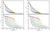 |
Fig. 1. Distortion coefficients cB (top panels) and cH (bottom panels) as functions of the baryonic mass M0 of models with a purely toroidal magnetic field (left panels) and with a purely poloidal magnetic field (right panels), for various value of β0: from β0 = − 6 (blue curve) to β0 = −4.5 (light red curve) increasing by 0.25 with every line. The red curve corresponds to GR. |
From a more quantitative point of view, the maximum relative difference between cB in GR and in STT in the purely toroidal case is roughly 63% for β0 = −6 and M0 ≈ 1.5 M⊙. This difference decreases approaching 0 as β0 increases. Moreover, as the baryonic mass increases, we can see that all sequences tend to coincide and reconnect to the GR one as the scalarisation range ends. As for cH, its maximum difference in STT relative to GR is roughly 72% at M0 ≈ 1.8 M⊙, for β0 = −6. Again, this difference decreases as β0 increases. We note, however, that the various sequences of cH do not seem to be reconnecting as the scalarisation range ends. This behaviour is to be attributed to the fact that the ratio  depends on M0, and, as such, it too exhibits the effect of scalarisation. In other words W̄, at a fixed M0, depends on β0, which implies that in STTs cH as defined in Eq. (6) is not directly comparable to GR at the same ℋ: first, it is needed to factor out the dependence of
  on M0 and add it to cH. The same holds for purely poloidal magnetic fields. The maximum relative difference of cB with respect to GR is 70% for β0 = −6 at M0 ≈ 1.5 M⊙, while for cH it is 72% at M0 ≈ 1.8 M⊙ for β0 = −6.
As we have seen, the distortion coefficients in STTs depart from the GR ones in a non-trivial way. Interestingly it looks like, apart from a scaling factor, both cH and cB have the same trend for toroidal and poloidal magnetic fields. In the case of cB, as can be seen from Fig. 1, for M0 < 1.6 M⊙, the values for toroidal magnetic fields are about a factor 1.5 higher than the cases with poloidal magnetic field. However, at higher masses, the trends are no longer similar between the two cases. Nonetheless, we have found that in the full range 1.2 ≤ M0/M⊙ ≲ 2.4 and −6 ≤ β0 ≤ −4.5, they are well approximated (to a few percents precision everywhere, except for the small range of masses in which scalarisation is triggered, where the error can reach a few tens of percents) by a combination of power laws of three global quantities defined for the corresponding unmagnetised model: the baryonic mass M0, the J-frame circumferential radius R̃c (see Eq. (C.8) in SBD20) and the E-frame scalar charge Q̄s (see Eq. (C.7) in SBD20). We note that these are not independent (for GR there is a one to one relation between mass and radius), but treating them as independent allows us to use simple power-law scalings in terms of global quantities. In particular:
![Mathematical equation: $$ \begin{aligned} c_\mathrm{B} \approx c_1 M_{1.6}^\alpha R_{10}^\beta \left[ 1-c_2 Q_{1}^\gamma M_{1.6}^\delta R_{10}^\rho \right] , \end{aligned} $$](/articles/aa/full_html/2021/01/aa38826-20/aa38826-20-eq24.gif) (7)
(7)
where the parameters are listed in Table 1, M1.6 is M0 in units of 1.6 M⊙, R10 is R̃c in units of 10 km, and Q1 is Q̄s in units of 1 M⊙. The first term of Eq. (7) describes the distortion coefficient in GR, while the second term describes the deviation due to the presence of a scalar charge. First, for the GR term, we note that the coefficient c1 of the models with toroidal field is about twice that of those with a poloidal one. The mass dependence is similar, while the exponent of the radius is higher by one for the poloidal field (this is likely due to the different geometry, prolate and oblate, of the configurations). From the coefficients in Table 1, we see that the second term of Eq. (7) has a more complex behaviour: the dependence on the scalar charge is similar, there is a weaker dependence on the mass for the poloidal field, while again the dependence on the radius is stronger by one power of R10 in the poloidal case. The similarity between NSs with poloidal and toroidal magnetic fields is much stronger for cH, to the point that it is possible to derive a universal functional form over the entire mass range with an accuracy of few percents:
 (8)
(8)
where ℱ(M0) represents the GR part and encodes the role of the equation of state,  represents the correction due to scalarisation, and the oblate versus prolate geometry induced by the different magnetic field is encoded in the last factor. We find that:
 (9)
(9)
 (10)
(10)
It is well known that in GR, the coefficient cH is only weakly dependent on the mass, to the point that it can almost be taken as a constant. This is because the specific properties of the NS cancel out if the deformation is given as a function of ℋ/W. What we found here is that the same holds in STTs. The deformation is smaller than in GR, but the functional form of the correction is independent of the specific STT. Moreover, the geometry of the magnetic field is completely encoded in a constant coefficient that likely traces the oblate or prolate geometry of the star.
Since a quadrupolar deformation of the NS results in the emission of quadrupolar waves, both tensor and scalar, it is interesting to analyse what fraction of the energy contained in them is due to the quadrupole moment of the scalar field. For this purpose, we define the following ratios:
 (11)
(11)
where
 (12)
(12)
![Mathematical equation: $$ \begin{aligned}&q_\mathrm{g} = \int \left[ \pi \mathcal{A} ^4 (\tilde{\varepsilon }+\tilde{\rho })-\frac{1}{8} (\partial \chi )^2 \right] r^4 \sin \theta \left(3\sin ^2\theta -2 \right) \mathrm{d} r \mathrm{d} \theta . \end{aligned} $$](/articles/aa/full_html/2021/01/aa38826-20/aa38826-20-eq31.gif) (13)
(13)
These are, respectively, the Newtonian approximations of the “trace quadrupole” and of the “mass quadrupole” of the NS. The mass quadrupole qg is just Īzz − Īxx = ēĪzz (see Eq. (4)). We found that, in the mass range we investigated, Īzz ranges from 6 × 1044 g cm2 to 4 × 1044 g cm2. This is consistent with GR, where the moment of inertia weakly depends on the mass (Lattimer & Prakash 2001), showing that the quadrupole is primarily encoded in the parameter ē. The quantities  and
and  are respectively the J-frame internal energy density and rest-mass density, while (∂χ)2 = (∂rχ)2 + r−2(∂θχ)2, and
  is qg calculated in GR. The quadrupole qs is closely related to the “quadrupolar deformation of the trace” (see SBD20, Eq. (C.19)), which acts as the source of scalar waves. We note that these scalar waves are of a quadrupolar nature and differ from standard scalar monopolar GWs, which we do not consider here. In fact, a monopolar scalar wave, being monopoles rotationally invariant, can only arise following time-dependent monopolar variations of the structure of the NS (e.g. when the star collapses, Gerosa et al. 2016) and is not triggered by the rotation of deformed NSs, to which our present results apply. This does not mean that rotation plays no role in monopolar waves emission since the vibrating eigenmodes depend on the NS structure, which also reflects the underlying rotational profile. We note that the distinction between monopolar and quadrupolar waves depends only on the energy distribution of the waves (the multipolar pattern of the radiation), while the distinction between scalar and tensor modes depends on the nature of the waves (the spin of the wave carriers). The quantity of 𝒮 gives a measure of which fraction of the energy lost in quadrupolar waves is contained in scalar modes, compared against tensor modes, while 𝒢 quantifies the ratio of the energy of tensor modes in STTs versus GR. We note that the tensor GW luminosity scales approximately with ē2, while it is the strain amplitude that scales with ē, so 𝒮 and 𝒢 are actually a measure of the variation in the strain, and it is their square to be related to the variation in the energy loss. It is worth pointing out that these ratios can be calculated by keeping fixed either B̃max or
  and that unlike B̃max,
  depends on M0 through W̄ in different ways for different theories of gravity. Let’s call this dependence f(M0, β0) in our case, where the difference between STT and GR is encoded only by a varying β0. This means that, in general, computing the ratios keeping fixed these two quantities does not yield the same result. In particular, ratios of quantities calculated with respect to models with the same β0, like 𝒮, are exactly the same in the two cases; instead, the ratio of a quantity in STTs over a quantity in GR, like 𝒢, differ by a factor f(M0, β0)/f(M0, 0).
In Fig. 2, we show the ratios in Eq. (11) for NSs endowed with a purely toroidal and a purely poloidal magnetic field, respectively. The top panels show that, when scalarisation occurs and 𝒮 departs from zero, very rapidly qs > qg for β0 ≲ −5, while sequences with β0 ≳ −5 do not reach 𝒮 = 1. This means that heavily scalarised NSs, once scalarisation kicks in, are dominated by losses due to scalar radiation, while less scalarised ones are always dominated by tensor radiation. Differences in 𝒮 between the purely toroidal and the purely poloidal cases are minimal, both in the scalarisation range and in the entity of its effect. The bottom panels of Fig. 2 show that once scalarisation is triggered, 𝒢 quickly falls down towards very low values; then, for NSs with a higher baryonic mass, 𝒢 rises again very steeply. At a fixed M0 below a threshold mass, the more scalarised the NS, the less energy is lost in tensor waves with respect to GR. On the other hand, the more scalarised the NS, the more energy is injected in the scalar mode channel, as shown before with the 𝒮 ratio, which increases almost monotonically with M0. However, more massive NSs have a quadrupole deformation that is closer to GR than less massive stars, which reflects in the rise of 𝒢 at high M0. For masses close to the maximum, tensor waves losses can be even higher than in GR. It is interesting to note that all sequences intersect the line 𝒢 = 1 at the same threshold mass M0 ≈ 1.85 M⊙. The reduction of the tensor GW strain is as high as 70% (75%) for M0 = 1.50 M⊙ (1.50 M⊙) for purely toroidal (poloidal) magnetic fields, for β0 = −6, while it is roughly 10% for M0 = 1.80 M⊙ and β0 = −4.5, for either purely toroidal or purely poloidal magnetic fields (see the blue and light red circles in Fig. 2). The same panels also show the ratio 𝒢 computed by keeping fixed  . We can see that, in this case, the drop and especially the subsequent rise are less steep; in the case of a purely poloidal magnetic field, 𝒢 is almost saturated to a constant value before slightly rising.
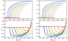 |
Fig. 2. Ratios 𝒮 (top panels) and 𝒢 (bottom panels) as functions of the baryonic mass M0 of models with a purely toroidal magnetic field (left panels) and with a purely poloidal magnetic field (right panels), for different value of β0: from β0 = −6 (blue curve) up to β0 = −4.5 (light red curve) increasing by 0.25 with every line. The red line corresponds to GR, where 𝒮 = 0 and 𝒢 = 1. Solid lines are the ratios computed by keeping B̃max fixed, while dashed lines are obtained by keeping |

As was done before with the distortion coefficient, we found that 𝒮 is well approximated (to a few percents precision everywhere but in the small range of masses where scalarisation occurs and the steepening is too strong to be well described by a simple power law) by
 (14)
(14)
for both the toroidal and the poloidal cases. This shows again that it is possible to find a unifying functional dependence, even for scalar modes. Also, the value of 𝒢 looks very similar for the poloidal and toroidal cases, except at the largest masses above 1.6 M⊙ (we note that being a ratio with respect to GR it can only be computed up to maximum GR mass). On the other hand, due to its more complex behaviour, we did not find a satisfying approximation for 𝒢 based on power laws of the quantities M0, Q̄s, R̃c.
It is evident that the power emitted in tensor modes by scalarised NSs is smaller, for masses below ≈1.85 M⊙, than for the model in GR of the same mass and same equation of state, even if the minimum does not correspond to the configuration with the strongest scalar charge. The trend changes for higher masses, where the losses in tensor modes in STTs are higher than for the corresponding GR models. Given that the scalar modes also contribute to the total energy losses, we see that as the mass rises, we first find a regime at the beginning of scalarisation, where the total GW emission is suppressed with respect to GR, which is then followed by a regime that is closer to the maximum mass where, due to the scalar channel, losses might even be enhanced by a factor of between 2 and 3.
The minimum value of 𝒢 (marked by the circles and squares in Fig. 2) scales quadratically, with β0 at fixed B̃max and  :
:
 (15)
(15)
and
 (16)
(16)
Analogously, the mass at which the minimum of 𝒢 occurs scales linearly with β0:
 (17)
(17)
and
 (18)
(18)
4. Conclusions
In this work we explore how the addition of a scalar field that is non-minimally coupled to the metric affects the magnetic quadrupolar deformation of a NS in the weak field regime (B̃max ≲ 1017 G). We find, as in Newtonian gravity and in GR, in this limit the quadrupolar deformation, ē, can be well-approximated by a linear function of either  or
or  , for fixed baryonic mass, M0, and scalarisation parameter, β0. We find that the coefficients of the linear expansion strongly depart from those of GR for sufficiently negative values of β0: for the range of parameters investigated here, spontaneous scalarisation can decrease the magnetic deformation of a NS by up to ≈70% of the GR value, for β0 = −6. For values of β0 ≳ −4.3, we find that the results in massless STTs without screening are indistinguishable from GR. This behaviour can be attributed to the interplay between various effects. First, given a certain EoS, we find that NSs in STTs have a different central density than those in GR with the same mass. In particular, below a threshold mass in the stable branch of the mass-central density diagram, scalarised models have a higher central density than the GR models with the same mass, which causes the inner region of the star to be less prone to deformation; the opposite happens for masses above the threshold, which are more susceptible to deformation than the corresponding GR models with the same mass. This tendency explains why 𝒢 is higher than unity for M0 ≳ 1.85 M⊙, which is very close to the threshold mass, which we found to be M0 ≈ 1.88 M⊙ for low magnetisations. Moreover, NSs endowed with a purely toroidal magnetic field have a prolate shape, with a more pronounced density gradient at the equator than at the pole, which, in turn, generates a steeper gradient of the scalar field at the equator than at the pole. Given that the effective pressure of the scalar field depends on its spatial derivatives and has the same sign as the fluid pressure, we see that its effect is to reduce the deformation of the star, making it more spherical. The same qualitative behaviour is exhibited by a star endowed with a purely poloidal magnetic field and which possesses an oblate shape with a steeper density gradient at the pole, thus causing the scalar field to apply more pressure in the polar direction than in the equatorial one. As expected, a more pronounced scalarisation (i.e. a more negative β0) reflects in a stronger pressure of the scalar field, rendering the star even more spherical, thus reducing the distortion coefficients further. It is known that the scalar field can act as a “stabiliser” for NSs, rendering their shape more spherical. Finally, the scalar field acts as an effective coupling term (it replaces the inverse of the gravitational constant of GR) between matter and the metric. In more scalarised systems, or in the NS central region where the scalar field is larger, this coupling is weaker, and this also holds for perturbations of the energy momentum tensor. Thus, the same structural deformation of the NS produces a weaker metric deformation. All these effects depend on where the deformation is located (centre versus the outer layers).
It is interesting to note that unlike the quadrupolar deformation of NSs caused by their rotation (see e.g. Doneva et al. 2014), the magnetic quadrupolar deformation, as we have seen, decreases in STTs with respect to GR, except for masses close to the maximum. This difference can be explained by the fact that rotation, unlike a magnetic field, affects mostly the outer layers of the NS, which in scalarised systems are less gravitationally bound than in GR (scalarized NS have larger radii than in GR), increasing their deformability with respect to GR. Magnetic deformation seems to be instead mostly regulated by the density in the central region where the magnetic field strength peaks.
Regarding GWs, STTs predict the existence of scalar waves, which, as we show here, can have an amplitude comparable to standard tensor waves and might even dominate the GW losses for strongly scalarised NSs. This can lead to a point when the total emission is even larger than in GR.
We find that a good approximation of the distortion coefficients is given by a simple power-law dependence on M0, R̃c, and Q̄s. More interestingly, we found that in terms of the ratio of magnetic to binding energy the effect of a scalar field on the NS deformation and the ratio of scalar to tensor waves emission can be parametrised by a unique function independently of the magnetic field structure or of the STT parameters. It seems that the presence of a scalar charge can easily be factorised. This is a generalisation of what was already known for GR, that is, with cH being almost a constant. As we described above, the magnetic deformability of NSs heavily depends on their internal structure, determined by the EoS. We leave to a future work to verify how much the functional form and the coefficients entering such function depend on the EoS.
Since the quadrupolar deformation of NSs, at a fixed M0 and for most of the scalarisation range, is reduced in STTs with respect to GR, it is expected that the energy lost in tensor GWs by deformed NSs is also reduced in STTs; on the other hand, it is enhanced for masses close to the maximum mass for a stable NS in GR. In fact, we found that strongly scalarised stars with a baryonic mass around 1.5 M⊙ have a tensor GW strain, h0, that is up to 75% lower than for the corresponding stars in GR, while it is roughly 10% lower, for β0 = −4.5, for masses of 1.8 M⊙. This means that, for values of β0 currently allowed by observations, a less than 10% variation in h0 is to be expected for massless scalar fields. This is much smaller than the typical uncertainties over the distances and the strength of magnetic fields, even for well-constrained galactic objects. Higher values might hold for massive scalar fields and this could lead to serious underestimations (or overestimations, depending on the mass) of the energetics of the system and all that follows from that, such as its distance or the strength of its magnetic field. If similar results on the role of the scalar field in the modification of tensor modes hold as well for other kinds of deformation (e.g. tidal deformations of scalarised NSs in mergers), this could have a deep impact on our understanding of binary NS merger events (Abbott et al. 2017). More interestingly, we found that the scalar mode can be emitted carrying an energy comparable to the tensor one. However, its strain is suppressed by a factor α0 ∼ 10−5 − 10−4, which weakens the coupling of the scalar mode to the detector and renders the possibility of it being detected even fainter.
Our results are computed in the full non-linear regime. We also computed the quadrupole deformation, holding both the metric and the scalar field fixed, which can be thought of as a Cowling approximation in STTs. In this case we found that for the mass range we investigated, the coefficients cB and cH are smaller by a factor ≈0.5−0.65.
The current sensitivities of the LIGO-Virgo observatories (Abbott et al. 2018) could be enough to detect tensor CGWs emitted by galactic neutrons stars remnants form merger events, with millisecond period (lasting few seconds), if the quadrupole deformation is e ≳ 10−5 (Lasky 2015; Abbott et al. 2020). Future GW detector of the class of Einstein Telescope (Punturo et al. 2010) and Cosmic Explorer (Reitze et al. 2019) could detect deformations as low as e ≳ 10−6. This means that, for what concerns continuous scalar waves, detectors with same sensitivity could reveal them from millisecond NSs, spinning for few seconds, only if the scalar quadrupole is  time bigger, which means magnetic field strength of the order of few 1017 G, at the limit of the values that can be reached (Ciolfi et al. 2019). For the same magnetic fields, tensor waves could be much more easily detected. Instead, the detection of scalar CGWs from slowly spinning magnetars with internal fields of few 1017 G (Olausen & Kaspi 2014; Thompson et al. 2020) requires instruments with a sensitivity at least one order of magnitude better than DECIGO (Kawamura et al. 2008) and BBO (Harry et al. 2006).
We caution the reader that there is evidence that the magnetic field at the surface or in the magnetosphere of NSs can have strong multipoles (Bignami et al. 2003; Bilous et al. 2019; Parthasarathy et al. 2020; Raynaud et al. 2020). However, the interpretation of the data is not unambiguous (e.g. the magnetic field inferred from cyclotron lines changes if either electron or proton cyclotron are assumed). It is even less clear how these apply to the magnetic field in the interior, whose geometry is totally unknown. From a theoretical point of view, it is reasonable to expect a difference between the interior and surface magnetic fields. The evolution of the latter is mostly dictated by the Hall term associated to crustal impurities, which leads to the formation of small-scale structures and higher order multipoles (Pons & Viganò 2019; De Grandis et al. 2020), while the dissipation of the former is mostly Ohmic, preferentially suppressing small-scale structure and higher multipoles (Haensel et al. 1990). Given that here we are mostly interested in the deviation with respect to GR, we can consider the purely toroidal and purely poloidal cases as two extrema of the much larger space of possible magnetic configurations. Our results showing that the deviations with respect to GR due to a scalar field are very similar in these two extrema lend us confidence to the consideration that similar deviations with respect to GR will also apply in more complex magnetic field geometries (Mastrano et al. 2013, 2015).
Acknowledgments
The authors also acknowledge financial support from the “Accordo Attuativo ASI-INAF n. 2017-14-H.0 Progetto: on the escape of cosmic rays and their impact on the background plasma” and from the INFN Teongrav collaboration.
References
- Abbott, B. P., Abbott, R., Abbott, T. D., et al. 2017, Phys. Rev. Lett., 119, 161101 [NASA ADS] [CrossRef] [PubMed] [Google Scholar]
- Abbott, B. P., Abbott, R., Abbott, T. D., et al. 2018, Liv. Rev. Rel., 21, 3 [NASA ADS] [CrossRef] [Google Scholar]
- Abbott, R., Abbott, T. D., Abraham, S., et al. 2020, ApJ, 902, L21 [CrossRef] [Google Scholar]
- Andersson, N.1998, ApJ, 502, 708 [NASA ADS] [CrossRef] [Google Scholar]
- Baym, G., Hatsuda, T., Kojo, T., et al. 2018, Rep. Prog. Phys., 81, 056902 [NASA ADS] [CrossRef] [Google Scholar]
- Bergmann, P. G.1968, Int. J. Theor. Phys, 1, 25 [CrossRef] [Google Scholar]
- Berti, E., Barausse, E., Cardoso, V., et al. 2015, CQG, 32, 243001 [CrossRef] [Google Scholar]
- Bignami, G. F., Caraveo, P. A., De Luca, A., & Mereghetti, S.2003, Nature, 423, 725 [NASA ADS] [CrossRef] [PubMed] [Google Scholar]
- Bilous, A. V., Watts, A. L., Harding, A. K., et al. 2019, ApJ, 887, L23 [CrossRef] [Google Scholar]
- Bocquet, M., Bonazzola, S., Gourgoulhon, E., & Novak, J.1995, A&A, 301, 757 [NASA ADS] [Google Scholar]
- Bonazzola, S., & Gourgoulhon, E.1996, A&A, 312, 675 [NASA ADS] [Google Scholar]
- Brans, C., & Dicke, R. H.1961, Phys. Rev., 124, 925 [NASA ADS] [CrossRef] [MathSciNet] [Google Scholar]
- Bucciantini, N., & Del Zanna, L.2011, A&A, 528, A101 [CrossRef] [EDP Sciences] [Google Scholar]
- Bucciantini, N., & Soldateschi, J.2020, MNRAS, 495, L56 [CrossRef] [Google Scholar]
- Bucciantini, N., Pili, A. G., & Zanna, L. D.2015, MNRAS, 447, 1 [CrossRef] [Google Scholar]
- Camelio, G., Dietrich, T., Marques, M., & Rosswog, S.2019, Phys. Rev. D, 100, 123001 [CrossRef] [Google Scholar]
- Capozziello, S., & de Laurentis, M.2011, Phys. Rep., 509, 167 [NASA ADS] [CrossRef] [MathSciNet] [Google Scholar]
- Ciolfi, R., Kastaun, W., Kalinani, J. V., & Giacomazzo, B.2019, Phys. Rev. D, 100, 023005 [CrossRef] [Google Scholar]
- Cordero-Carrión, I., Cerdá-Durán, P., Dimmelmeier, H., et al. 2009, Phys. Rev. D, 79, 024017 [NASA ADS] [CrossRef] [Google Scholar]
- Cutler, C.2002, Phys. Rev. D, 66, 084025 [NASA ADS] [CrossRef] [Google Scholar]
- Dall’Osso, S., Shore, S. N., & Stella, L.2009, MNRAS, 398, 1869 [NASA ADS] [CrossRef] [Google Scholar]
- Damour, T., & Esposito-Farèse, G.1993, Phys. Rev. Lett., 70, 2220 [NASA ADS] [CrossRef] [Google Scholar]
- De Grandis, D., Turolla, R., Wood, T. S., et al. 2020, ApJ, 903, 40 [CrossRef] [Google Scholar]
- Del Zanna, L., & Bucciantini, N.2018, MNRAS, 479, 657 [NASA ADS] [Google Scholar]
- Doneva, D. D., & Yazadjiev, S. S.2016, JCAP, 2016, 019 [CrossRef] [Google Scholar]
- Doneva, D. D., Yazadjiev, S. S., Staykov, K. V., & Kokkotas, K. D.2014, Phys. Rev. D, 90, 104021 [CrossRef] [Google Scholar]
- Franceschetti, K., & Del Zanna, L.2020, Universe, 6, 83 [CrossRef] [Google Scholar]
- Frieben, J., & Rezzolla, L.2012, MNRAS, 427, 3406 [NASA ADS] [CrossRef] [Google Scholar]
- Fujii, Y., & Maeda, K.-I.2003, The Scalar-Tensor Theory of Gravitation, Cambridge Monographs on Mathematical Physics (Cambridge University Press) [CrossRef] [Google Scholar]
- Gerosa, D., Sperhake, U., & Ott, C. D.2016, CQG, 33, 135002 [CrossRef] [Google Scholar]
- Gourgoulhon, E.2010, CompStar 2010: School and Workshop on Computational Tools for Compact Star Astrophysics [Google Scholar]
- Haensel, P., Urpin, V. A., & Yakovlev, D. G.1990, A&A, 229, 133 [NASA ADS] [Google Scholar]
- Harry, G., Fritschel, P., Shaddock, D., Folkner, W., & Phinney, E.2006, CQG, 23, 4887; Erratum: Class. Quant. Grav., 23, 7361 (2006) [CrossRef] [Google Scholar]
- Haskell, B., Jones, D. I., & Andersson, N.2006, MNRAS, 373, 1423 [NASA ADS] [CrossRef] [Google Scholar]
- Hawking, S. W.1972, Commun. Mat. Phys., 25, 167 [CrossRef] [MathSciNet] [Google Scholar]
- Iosif, P., & Stergioulas, N.2014, Gen. Relativ. Grav., 46, 1800 [CrossRef] [Google Scholar]
- Kawamura, S., Ando, M., Nakamura, T., et al. 2008, J. Phys. Conf. Ser., 122, 012006 [CrossRef] [Google Scholar]
- Keer, L., & Jones, D. I.2015, MNRAS, 446, 865 [CrossRef] [Google Scholar]
- Kiuchi, K., & Yoshida, S.2008, Phys. Rev. D, 78, 044045 [NASA ADS] [CrossRef] [Google Scholar]
- Lasky, P. D.2015, PASA, 32, e034 [CrossRef] [Google Scholar]
- Lattimer, J., & Prakash, M.2007, Phys. Rep., 442, 109 [NASA ADS] [CrossRef] [Google Scholar]
- Lattimer, J. M., & Prakash, M.2001, ApJ, 550, 426 [NASA ADS] [CrossRef] [Google Scholar]
- Mastrano, A., Lasky, P. D., & Melatos, A.2013, MNRAS, 434, 1658 [NASA ADS] [CrossRef] [Google Scholar]
- Mastrano, A., Suvorov, A. G., & Melatos, A.2015, MNRAS, 447, 3475 [CrossRef] [Google Scholar]
- Matsuda, T., & Nariai, H.1973, Prog. Theor. Phys., 49, 1195 [CrossRef] [Google Scholar]
- Melatos, A., & Payne, D. J. B.2005, ApJ, 623, 1044 [NASA ADS] [CrossRef] [Google Scholar]
- Metzger, B. D., Giannios, D., Thompson, T. A., Bucciantini, N., & Quataert, E.2011, MNRAS, 413, 2031 [NASA ADS] [CrossRef] [Google Scholar]
- Novak, J.1998, Phys. Rev. D, 57, 4789 [CrossRef] [Google Scholar]
- Olausen, S. A., & Kaspi, V. M.2014, ApJS, 212, 6 [Google Scholar]
- Ostriker, J. P., & Gunn, J. E.1969, ApJ, 157, 1395 [NASA ADS] [CrossRef] [Google Scholar]
- Pang, P. T. H., Lo, R. K. L., Wong, I. C. F., Li, T. G. F., & Van Den Broeck, C.2020, Phys. Rev. D, 101, 104055 [CrossRef] [Google Scholar]
- Pani, P., & Berti, E.2014, Phys. Rev. D, 90, 024025 [CrossRef] [Google Scholar]
- Parthasarathy, A., Johnston, S., Shannon, R. M., et al. 2020, MNRAS, 494, 2012 [CrossRef] [Google Scholar]
- Pili, A. G., Bucciantini, N., & Del Zanna, L.2014, MNRAS, 439, 3541 [CrossRef] [Google Scholar]
- Pili, A. G., Bucciantini, N., & Del Zanna, L.2015, MNRAS, 447, 2821 [CrossRef] [Google Scholar]
- Pili, A. G., Bucciantini, N., & Del Zanna, L.2017, MNRAS, 470, 2469 [CrossRef] [Google Scholar]
- Pons, J. A., & Viganò, D.2019, Liv. Rev. Comput. Astrophys., 5, 3 [CrossRef] [Google Scholar]
- Punturo, M., Abernathy, M., Acernese, F., et al. 2010, CQG, 27, 194002 [Google Scholar]
- Raynaud, R., Guilet, J., Janka, H.-T., & Gastine, T.2020, Sci. Adv., 6, 2732 [NASA ADS] [CrossRef] [Google Scholar]
- Reitze, D., Adhikari, R. X., Ballmer, S., et al. 2019, BAAS, 51, 35 [NASA ADS] [Google Scholar]
- Rowlinson, A., O’Brien, P. T., Metzger, B. D., Tanvir, N. R., & Levan, A. J.2013, MNRAS, 430, 1061 [NASA ADS] [CrossRef] [Google Scholar]
- Santiago, D. I., & Silbergleit, A. S.2000, Gen. Relativ. Grav., 32, 565 [CrossRef] [Google Scholar]
- Shao, L., Sennett, N., Buonanno, A., Kramer, M., & Wex, N.2017, Phys. Rev. X, 7, 041025 [Google Scholar]
- Shibata, M., Taniguchi, K., Okawa, H., & Buonanno, A.2014, Phys. Rev. D, 89, 084005 [CrossRef] [Google Scholar]
- Soldateschi, J., Bucciantini, N., & Del Zanna, L.2020, A&A, 640, A44 [CrossRef] [EDP Sciences] [Google Scholar]
- Sotani, H., & Kokkotas, K. D.2005, Phys. Rev. D, 71, 124038 [CrossRef] [Google Scholar]
- Thompson, K. L., Frederick, S. G., & Kuchera, M. P.2020, ArXiv e-prints [arXiv:2002.02619] [Google Scholar]
- Ushomirsky, G., Cutler, C., & Bildsten, L.2000, MNRAS, 319, 902 [NASA ADS] [CrossRef] [Google Scholar]
- Voisin, G., Cognard, I., Freire, P. C. C., et al. 2020, A&A, 638, A24 [CrossRef] [EDP Sciences] [Google Scholar]
- Wagoner, R. V.1970, Phys. Rev. D, 1, 3209 [NASA ADS] [CrossRef] [Google Scholar]
- Wentzel, D. G.1960, ApJS, 5, 187 [NASA ADS] [CrossRef] [Google Scholar]
- Will, C. M.2014, Liv. Rel. Rev., 17, 4 [NASA ADS] [CrossRef] [PubMed] [Google Scholar]
- Zhang, X., Niu, R., & Zhao, W.2019, Phys. Rev. D, 100, 024038 [CrossRef] [Google Scholar]
All Tables
All Figures
|
Fig. 1. Distortion coefficients cB (top panels) and cH (bottom panels) as functions of the baryonic mass M0 of models with a purely toroidal magnetic field (left panels) and with a purely poloidal magnetic field (right panels), for various value of β0: from β0 = − 6 (blue curve) to β0 = −4.5 (light red curve) increasing by 0.25 with every line. The red curve corresponds to GR. |
| In the text | |
|
Fig. 2. Ratios 𝒮 (top panels) and 𝒢 (bottom panels) as functions of the baryonic mass M0 of models with a purely toroidal magnetic field (left panels) and with a purely poloidal magnetic field (right panels), for different value of β0: from β0 = −6 (blue curve) up to β0 = −4.5 (light red curve) increasing by 0.25 with every line. The red line corresponds to GR, where 𝒮 = 0 and 𝒢 = 1. Solid lines are the ratios computed by keeping B̃max fixed, while dashed lines are obtained by keeping |
| In the text | |
Current usage metrics show cumulative count of Article Views (full-text article views including HTML views, PDF and ePub downloads, according to the available data) and Abstracts Views on Vision4Press platform.
Data correspond to usage on the plateform after 2015. The current usage metrics is available 48-96 hours after online publication and is updated daily on week days.
Initial download of the metrics may take a while.