| Issue |
A&A
Volume 694, February 2025
|
|
|---|---|---|
| Article Number | A39 | |
| Number of page(s) | 13 | |
| Section | Astrophysical processes | |
| DOI | https://doi.org/10.1051/0004-6361/202451904 | |
| Published online | 31 January 2025 | |
Reality of inverse cascading in neutron star crusts
1
Departament de Física Aplicada, Universitat d’Alacant, Ap. Correus 99, E-03080 Alacant, Spain
2
Nordita, KTH Royal Institute of Technology and Stockholm University, 10691 Stockholm, Sweden
3
The Oskar Klein Centre, Department of Astronomy, Stockholm University, AlbaNova, SE-10691 Stockholm, Sweden
4
McWilliams Center for Cosmology & Department of Physics, Carnegie Mellon University, Pittsburgh, PA 15213, USA
5
School of Natural Sciences and Medicine, Ilia State University, 3-5 Cholokashvili Avenue, 0194 Tbilisi, Georgia
⋆ Corresponding author; This email address is being protected from spambots. You need JavaScript enabled to view it.
Received:
16
August
2024
Accepted:
9
January
2025
Abstract
The braking torque that dictates the timing properties of magnetars is closely tied to the large-scale dipolar magnetic field on their surface. The formation of this field has been a topic of ongoing debate. One proposed mechanism, based on macroscopic principles, involves an inverse cascade within the neutron star’s crust. However, this phenomenon has not been observed in realistic simulations. In this study, we provide compelling evidence supporting the feasibility of the inverse cascading process in the presence of an initial helical magnetic field within realistic neutron star crusts and discuss its contribution to the amplification of the large-scale magnetic field. Our findings, derived from a systematic investigation that considers various coordinate systems, peak wavenumber positions, crustal thicknesses, magnetic boundary conditions, and magnetic Lundquist numbers, reveal that the specific geometry of the crustal domain–with its extreme aspect ratio–requires an initial peak wavenumber from small-scale structures for the inverse cascade to occur. However, this same aspect ratio confines the cascade to structures on the scale of the crust, making the formation of a large-scale dipolar surface field unlikely. Despite these limitations, the inverse cascade remains a significant factor in the magnetic field evolution within the crust and may help explain highly magnetized objects with weak surface dipolar fields, such as low-field magnetars and central compact objects.
Key words: magnetic fields / stars: evolution / stars: interiors / stars: magnetars / stars: magnetic field / stars: neutron
© The Authors 2025
 Open Access article, published by EDP Sciences, under the terms of the Creative Commons Attribution License (https://creativecommons.org/licenses/by/4.0), which permits unrestricted use, distribution, and reproduction in any medium, provided the original work is properly cited.
This article is published in open access under the Subscribe to Open model. This email address is being protected from spambots. You need JavaScript enabled to view it. to support open access publication.
1. Introduction
Magnetars are the most magnetic objects within the population of neutron stars (NSs) (Turolla et al. 2015; Esposito et al. 2021). Their bright X-ray luminosity and occurrence of observed bursts and outbursts are attributed to the restless dynamics and dissipation of a strong magnetic field (about 1014 to 1015 G) near the NS surface (Thompson & Duncan 1995). Moreover, the large-scale dipolar field on the surface regulates the braking torque responsible for their timing properties (Ostriker & Gunn 1969), resulting in long spin-periods.
The origin and evolution of NS magnetic fields have been long-debated topics. While it is widely accepted that the fossil magnetic field inherited from the progenitor star is insufficient to account for the strongest observed NS fields, additional amplification is necessary. This amplification might occur during the proto-NS stage through a turbulent dynamo process (Balbus & Hawley 1991; Obergaulinger et al. 2014; Raynaud et al. 2020; Reboul-Salze et al. 2021; Aloy & Obergaulinger 2021). Magnetic field amplification can also take place later in an NS’s life, for instance due to the re-emergence of a buried magnetic field driven by Hall drift (see Igoshev et al. 2021 for a review), or through the chiral magnetic instability (CMI) in the NS crust, a microscopic-based mechanism that can explain the formation of large-scale magnetic fields (Dehman & Pons 2024).
Understanding the amplification of the surface dipolar field in magnetars is a challenging task, where macroscopic mechanisms like inverse cascading could be important phenomena to consider. A recent attempt to explain this phenomenon, utilizing an initial turbulent field structure derived from proto-NS dynamo simulations (Reboul-Salze et al. 2021), is presented in Dehman et al. (2023a). The authors conducted the first 3D coupled magneto-thermal simulation in the crust of a NS, incorporating temperature-dependent microphysical calculations and a realistic stellar structure. The study aimed to determine if starting from such an initial field configuration could explain the observed dipolar field in magnetars. While successful in explaining the characteristic energy spectrum of low-field magnetars, high-field pulsars, and central compact objects (CCOs), this study falls short in explaining the strong surface dipolar field observed in magnetars. The surface dipolar component remained constant over time, with no evidence of an inverse cascade. Other simulations dedicated to the investigation of CCOs have also sought to observe inverse cascading, as seen in Gourgouliatos et al. (2020). Although they did find a substantial increase of the dipole component of the magnetic field, the location of the peak of the spectrum remained unchanged. Because of this, they concluded that their simulations showed no signs of a true inverse cascade.
Earlier work by Wareing & Hollerbach (2009, 2010) and Cho (2011) identified the role of magnetic helicity in driving an inverse cascade under the influence of Hall drift. An inverse cascade was known to exist in magnetohydrodynamics with helical driving (Frisch et al. 1975). Building on those findings, recent local simulations of the Hall cascade with initial magnetic helicity were presented by Brandenburg (2020). This model was later applied to simulate the evolution of a population of NSs (Sarin et al. 2023). In the study by Brandenburg (2020), the author proposed a model suggesting that the large-scale magnetic field of NSs grows as a result of small-scale turbulence. Initially, the magnetic field in young NSs may predominantly exist at small scales, but it could later undergo an inverse cascade, particularly after the crust solidifies. This process implies that the spectral magnetic energy at lower multipoles would increase over time rather than decrease. The study further demonstrates that the resulting dipolar field intensifies approximately linearly with time, typically growing by three orders of magnitude, while thermal dissipation gradually diminishes.
As explained by Brandenburg (2020), the presence of an initial helical magnetic field could be a key factor behind the observed phenomenon of inverse cascading. The simulations further suggest that, even with a relatively weak initial magnetic field, the occurrence of strong inverse cascading is evident. There are two possible sources of magnetic helicity in a NS. One is through dynamo action by neutrino-driven convection in young NS, resulting in oppositely signed magnetic helicities in the two hemispheres (Thompson & Duncan 1995; Brandenburg & Subramanian 2005). Another possible origin of helical magnetic fields in NSs is the CMI. This effect is significant during supernova explosions, throughout the proto-NS phase, and in young NSs. The CMI influences the evolution of the magnetic field in these compact objects, leading to the saturation of magnetic helicity. This, in turn, results in the growth of magnetic fields, which is governed by a conservation law for total chirality (Sigl & Leite 2016; Rogachevskii et al. 2017; Schober et al. 2018; Masada et al. 2018; Brandenburg et al. 2023a,b; Dehman & Pons 2024). Consequently, adopting an initial helical magnetic field provides a realistic foundation for modeling the long-term evolution of NS magnetic fields.
In addition to the significance of the initial helical field in explaining the phenomenon of inverse cascading, several other factors play a crucial role in comprehending the occurrence of inverse cascading within a realistic NS crust. Building upon the findings of Brandenburg (2020), where inverse cascading was first observed in the NS crust, several extensions can be explored. These include incorporating a spherical shell geometry, accounting for the precise aspect ratio determined by applying the Tolman-Oppenheimer-Volkoff equation (Oppenheimer & Volkoff 1939) and employing a realistic nuclear matter equation of state (EoS). Furthermore, instead of imposing periodic boundary conditions, alternative boundary conditions can be considered. Options such as potential boundary conditions at the surface and perfect conductor at the crust-core interface may provide valuable insights. However, at the surface of the star, the most suitable boundary conditions are force-free ones (Akgün et al. 2018; Urbán et al. 2023). Finally, within the NS, the stratification of matter is a crucial consideration. The inclusion of density- and temperature-dependent microphysics becomes imperative for accurately computing the Hall prefactor and magnetic diffusivity employed in the evolution equations.
In this article, we aim to explore the potential occurrence of inverse cascading in the crust of a NS by simulating a realistic NS scenario. Our objective is to understand the role of inverse cascading in explaining the strong surface dipole field observed in magnetars. Additionally, we seek to address why this phenomenon has not been identified in previous studies within the NS community. We investigate this process over a time span of 103 to 105 years, corresponding to the observed lifetime of magnetars. To achieve these goals, we employ both the PENCIL CODE1 (Pencil Code Collaboration 2021) and MATINS (Dehman et al. 2023b), taking into account the various relevant parameters.
This paper is organized as follows: In Sect. 2, we discuss the theoretical formalism of magnetic helicity and its realizability conditions in both Cartesian and spherical coordinates. The numerical setups and the initial conditions are described in Sect. 3. The results of our simulations are presented in Sect. 4, and we conclude with a discussion of our findings in Sect. 5.
2. Magnetic helicity and realizability condition
2.1. General considerations
As previously noted, a helical magnetic field plays an important role in explaining inverse cascading, which might be considered as a candidate to explain the large-scale dipolar field in magnetars. The idea of explaining inverse cascading using a helical field was first proposed by Frisch et al. (1975). The first application to NS physics was explored by Brandenburg (2020). The idea is based on the conservation of magnetic helicity,
 (1)
(1)
where A is the magnetic vector potential and B = ∇ × A is the magnetic field in a volume V.
Following Brandenburg (2020), simple coordinate-independent measures related to magnetic helicity can be defined in terms of the fractional helicity χ and the length scale ξ, which are introduced through the ratios
 (2)
(2)
Here, J = ∇ × B/μ0 is the current density, where μ0 is the vacuum permeability (in practice, we often use units such that μ0 = 1). Angle brackets denote averages over closed volumes, so ⟨A ⋅ B⟩ is gauge-invariant. These relations yield χ2 = μ0⟨A ⋅ B⟩⟨J ⋅ B⟩/⟨B2⟩2, from which the fractional magnetic helicity χ is determined.
We recall that for a fully helical Beltrami field with periodic boundary conditions, we have χ = 1. When the boundary conditions are nonperiodic, for example perfectly conducting on one side and a vertical field condition on the other, Brandenburg (2017) determined analytically the quantity ϵm ≡ ⟨J ⋅ B⟩/(⟨J2⟩⟨B2⟩)1/2 ≈ 0.883, which also implies χ = 0.883, because in his case ⟨J ⋅ B⟩/⟨A ⋅ B⟩ = μ0⟨J2⟩/⟨B2⟩. Thus, χ can be close to unity even in the nonperiodic case. Furthermore, because χ is only an approximate quantity, it can sometimes also exceed unity by a certain amount (Brandenburg 2020).
The χ approach provides a practical alternative to more rigorous methods that are typically feasible in Cartesian coordinates, which will be discussed next. Using χ, when treated as position-dependent, is also a useful tool if the magnetic diffusivity and/or the Hall prefactor vary with depth (see Brandenburg 2020, for examples). However, in order to clarify the viability of an inverse cascade in spherical geometry, such variations will be ignored in the present paper.
2.2. Cartesian coordinates
Assuming periodic boundary conditions, the spectra of magnetic energy and magnetic helicity, EM(k) and HM(k), can be computed by calculating the three-dimensional Fourier transforms of the magnetic vector potential  and the magnetic field
  . The spectra are obtained by integrating
  and the real part of
  over shells of constant k = |k|, yielding EM(k) and HM(k), respectively. Here, the asterisk denotes complex conjugation. These spectra are normalized such that ∫EM(k) dk = ⟨B2⟩/2μ0 and ∫HM(k) dk = ⟨A ⋅ B⟩ for k from 0 to ∞. By applying the Schwartz inequality, one can derive the so-called realizability condition (Moffatt 1978),
 (3)
(3)
The realizability condition serves as an indicator of the degree of helicity within the magnetic field. When Eq. (3) is saturated at a particular wavenumber k, the magnetic helicity is maximal at that wavenumber. If this condition holds true for any arbitrary k, the system is characterized as being in a state of maximal helicity (Frisch et al. 1975).
For fully helical magnetic fields with (say) positive helicity (e.g., HM = 2μ0EM(k)/k), Frisch et al. (1975) demonstrated that energy and magnetic helicity cannot cascade directly. Specifically, the interaction of modes with wavenumbers p and q produces fields whose wavevector k = p + q has a length that is equal to or smaller than the maximum of either |p| or |q| (Brandenburg & Subramanian 2005), expressed as
 (4)
(4)
This implies that magnetic helicity and magnetic energy transform into progressively larger length scales, defining what is known as the inverse cascade. Consequently, the entire spectrum is expected to shift leftward, toward larger length scales, in an approximately self-similar fashion (Brandenburg & Kahniashvili 2017).
For the decay of a fully helical magnetic field, the height of the spectrum  remains unchanged. This is because the typical length scale ξ increases (k ∝ 1/ξ decreases for a fully helical field; see Eq. (4)), but the mean magnetic helicity density ⟨A ⋅ B⟩ ≈ ξ⟨B2⟩ is constant, so the mean magnetic energy density
  must decrease such that
  stays constant. Thus, the constancy of the height of the spectrum in the case of a fully helical field does not indicate that the mean magnetic energy density is constant during the evolution.
2.3. Spherical coordinates
In spherical coordinates, B can be expressed using two scalar functions Φ(x) and Ψ(x), following the Chandrasekhar-Kendall formulation (Chandrasekhar & Kendall 1957; Chandrasekhar 1981):
 (5)
(5)
Using the notation of Krause & Rädler (1980) and Geppert & Wiebicke (1991), the basic idea is to expand the poloidal Φ and toroidal Ψ scalar functions in a series of spherical harmonics:
 (6)
(6)
where ℓ = 1 to ∞ is the degree and m = −ℓ,…,ℓ the order of the multipole. The toroidal field in 3D is a mix of the two tangential components of the magnetic field, whereas the poloidal field is a mix of all three components. This is less trivial than in 2D, where the toroidal part consists of the azimuthal component and the poloidal part consists of the two other components of the magnetic field.
The spectra of the magnetic helicity and the magnetic energy in 3D spherical coordinates are, respectively, defined as follows:
 (7)
(7)
![Mathematical equation: $$ \begin{aligned}&E_{\rm M}(\ell ,m;t) = \frac{1}{2} \int \frac{\ell (\ell +1)}{r^2} \bigg [\frac{\ell (\ell +1)}{r^2} \Phi _{\ell m}^2 +\Phi ^\prime _{\ell m} \,^2 +\Psi _{\ell m}^2\bigg ]. \end{aligned} $$](/articles/aa/full_html/2025/02/aa51904-24/aa51904-24-eq15.gif) (8)
(8)
Here, Φ′ℓm = ∂Φℓm/∂r. From these expressions, one can define the spectral realizability condition (Eq. (3)) in terms of the poloidal and toroidal scalar functions as
 (9)
(9)
The pseudo wavenumber  possesses the dimension of inverse length, where R denotes the surface of our computational domain.
3. Numerical models
3.1. Evolution equations
Using SI units, the equations governing the Hall cascade in NS crust can be written as (Goldreich & Reisenegger 1992)
 (10)
(10)
where e is the unit charge, ne is the electron density, and η is the magnetic diffusivity (inversely proportional to the electrical conductivity σe).
A suitable adimensional measure quantifying the importance of magnetic diffusivity is the Lundquist number, given by
 (11)
(11)
Owing to the decay of Brms, the value of Lu is time-dependent. Additionally, it exhibits positional dependence because ne and η vary with density. However, this positional dependence is not addressed in the present study.
3.2. Numerical codes
As mentioned above, we use two numerical codes: the PENCIL CODE2 (Pencil Code Collaboration 2021) and MATINS (Dehman et al. 2023b). The PENCIL CODE is primarily designed to solve the fully nonlinear, compressible hydromagnetic equations. Its highly modular structure allows for easy adaptation to a wide range of physical setups. It is a high-order finite-difference code, which is efficiently parallelized, enabling therefore high resolution and Lundquist numbers on the order of 103. The code can operate on a Cartesian or spherical grid and can be configured to work within a limited sector, θ1 ≤ θ ≤ θ2 and ϕ1 ≤ ϕ ≤ ϕ2, of a 3D spherical shell. This capability allows us to exclude the axis to avoid singularities and to adjust the aspect ratio as needed. Therefore, the PENCIL CODE is a valuable tool for this study.
On the other hand, MATINS is a 3D code for the MAgneto-Thermal evolution in Isolated NS crusts, based on finite-volume numerical schemes discretized over a nonorthogonal cubed-sphere grid, which effectively resolves the axis singularity problem in 3D spherical coordinates. The cubed-sphere formalism, introduced by Ronchi et al. (1996) and implemented in MATINS by Dehman et al. (2023b), uses one coordinate as the radial direction, similar to spherical coordinates, with the volume composed of multiple radial layers. Each layer is divided into six patches, resembling arcs of great circles, created by inflating the six faces of a cube into a spherical shape. Each patch is bordered by four others and is described by angular-like coordinates, ξcs and ηcs, ranging from [ − π/4 : π/4]. These patches are orthogonal to the radial direction but not orthogonal to each other, except at the patch centers. This nonorthogonality requires careful distinction between covariant (lower indices) and contravariant (upper indices) field components.
Additionally, MATINS incorporates a spherical star based on a realistic EoS, including corresponding relativistic factors in the evolution equations. It also integrates the latest temperature-dependent microphysical calculations3, enabling coupled magneto-thermal simulations if needed (Dehman et al. 2023a,b; Ascenzi et al. 2024).
3.3. Initial conditions
In the following, our objective is to construct an initial helical magnetic field. We use a random initial field with a specific magnetic energy spectrum. It peaks at a certain wavenumber k0. For wavenumbers k > k0, the spectrum exhibits a distinct inertial range, which may follow a k−5/3 scaling for Kolmogorov-like turbulence or a k−2 scaling for wave turbulence (Brandenburg et al. 2015). For k < k0, referred to as the sub-inertial range, we adopt a spectrum corresponding to a random vector potential. This implies that in 3D space, the vector potential follows a k2 spectrum and the magnetic field a k4 spectrum, as depicted in Table 1. Such a spectrum is often used in the cosmological context, where it is usually referred to as a causal spectrum (Durrer & Caprini 2003). It means that no point is correlated with any other, but the field is additionally divergence-free.
Spectrum of the magnetic vector potential A and the magnetic field B for k ≪ k0, depicting the ascending spectra.
3.3.1. The Pencil Code
In Cartesian coordinates, we use a Fourier transform to construct a helical initial condition for the magnetic vector potential A(k) by applying the helicity operator  with unit vector
  on a nonhelical transverse field given by:
 (12)
(12)
Here, A0 is an amplitude factor, φ with |φ|< π are uniformly distributed random phases, and
![Mathematical equation: $$ \begin{aligned} {S\!}_A(k)= \frac{k_0^{-3/2} (k/k_0)^{\alpha /2-2}}{\big [1+ (k/k_0)^{2(\alpha +7/3)}\big ]^{1/4}}\cdot \end{aligned} $$](/articles/aa/full_html/2025/02/aa51904-24/aa51904-24-eq23.gif) (13)
(13)
is a function that gives EM(k)∝kα for k ≪ k0 and EM(k)∝k−7/3 for k ≫ k0. For more details on how α scales with the dimension of the domain, we refer to Table 1 and to the work of Brandenburg & Boldyrev (2020). Here, k0 is the peak wavenumber of the spectrum. For a given value of B0, the resulting initial value of the rms magnetic field, Brms, which will be denoted as  , is usually somewhat larger than B0. For k0/k1 = 180, for example, we find
  when σ = 0, and
  when σ = 1.
Owing to the use of Fourier transforms, our initial conditions are implicitly assumed to be triply periodic in x, where x = (x, y, z) with x1 < x < x2, y1 < y < y2, and z1 < z < z2. The boundary conditions imposed during the simulation may lead to sharp gradients at the boundaries during the initial time steps, but those will be smoothed out later in time.
When using the PENCIL CODE, we can still use the Cartesian initial condition in spherical geometry by replacing (x, y, z)→(r, θ, ϕ). In that case, the vector potential will no longer be perfectly divergence-free. Also, in the simulations, we are not working in the Coulomb gauge; instead, we employ the Weyl gauge where the electrostatic potential vanishes. Additionally, the fractional magnetic helicity will be different in this scenario (see Sect. 2 for coordinate-independent measures of the fractional magnetic helicity).
In the following, we characterize the surface magnetic field in the Cartesian simulations through its two-dimensional energy spectrum, EM(k; x, t), where k = |k| and k = (ky, kz) is the wavevector in the yz plane. We choose a value of x that is close to the outer boundary, x2 (beneath the star’s surface). Owing to the reduction in dimensionality, the otherwise k4 spectrum of the magnetic field turns into a k3 spectrum (see Table 1).
3.3.2. The MATINS code
According to the Chandrasekhar-Kendall formalism (Chandrasekhar & Kendall 1957), the magnetic field B can be decomposed in spherical coordinates, into poloidal Φ(x) and toroidal Ψ(x) scalar functions, as explained in Sect. 2.3. The initial magnetic field structure can be constructed by selecting a set of spherical harmonics (see Eq. (6)), which defines the angular part of the magnetic field configuration. For additional details, consult Appendix B of Dehman et al. (2023b).
As mentioned at the beginning of Sect. 3.3, our goal is to start the simulations with a locally isotropic spectrum characterized by an ℓ3 slope4. Thus, we express the poloidal scalar function Φ(x) as:
 (14)
(14)
with
 (15)
(15)
Here, Φℓm(ra) represents the weights of the multipoles, extracted from simulations using the PENCIL CODE at a given radial layer ra beneath the surface of the star R. The surface differential is denoted by dSr, fℓ(r) is the radial spectral mode function, and Br is the contravariant radial component of the magnetic field, as MATINS employs a nonorthogonal cubed-sphere metric. This selection ensures the achievement of the desired locally isotropic ℓ3 initial sub-inertial range.
To establish a locally isotropic magnetic field across all radial layers, we define fℓ(r) as follows:
 (16)
(16)
where kℓeff is the radial wavenumber. The choice of kℓeff is motivated by the dimensional argument of the realizability condition; see Eqs. (3) and (9). The parameter ι is a constant that can be adjusted in our simulations to ensure the desired number of multipoles along the radial direction, as one can define k0R ∝ ι ℓ0. Here, k0 and ℓ0 are the peak wavenumber and degree of the multipoles in the spectrum, respectively. For ι = 1, kℓeff simplifies to the wavenumber k. We refer to Sect. 4.2 for details regarding the selection of the ι parameter.
The choice of the radial spectral mode function fl(r), as defined, does not adhere to the potential and perfect conductor boundary conditions imposed at the surface and the crust-core boundary, respectively. However, considering our goal of conducting simulations with a large Lundquist number on the order of 100 − 1000, it is anticipated that the initial condition’s influence on the global evolution will be minimal. Also, as discussed above, the magnetic field is expected to readjust to the imposed boundary conditions after a few evolution time steps, a behavior also observed in the PENCIL CODE simulations. It is worth noting that, in order to construct an initial field that respects boundary conditions, the solution of Bessel functions would be necessary, which inspired our current choice of the sine function.
To construct an initial helical field, the toroidal scalar function Ψ(x) must be expressed as
 (17)
(17)
where  . Upon examining Equation (9), it becomes apparent that, at the surface of the star, the ratio of the left-hand side to the right-hand side approaches one, indicating that the magnetic field tends toward maximal helicity. However, the presence of the
  term on the right-hand side of Equation (9) prevents the Chandrasekhar-Kendall formalism from achieving a fully helical field. It is worth noting that different choices of the radial function also ensure a helical field if Equation (17) is enforced.
The magnetic field components are computed using the finite-volume curl operator applied to Φ(x) and Ψ(x) in cubed-sphere coordinates; see Dehman et al. (2023b). This method guarantees that the initial magnetic field structure is divergence-free up to machine precision and effectively avoids the axis-singularity problem inherent in spherical coordinate. Our experience shows that this approach yields satisfactory results for our objectives, particularly in generating a visually more locally isotropic field, as will be demonstrated in Sect. 4.
3.4. Boundary conditions
In our simulations, we confine the magnetic field to the crust of the star. Consequently, the inner boundary conditions are imposed by requiring the normal (radial) component of the magnetic field to vanish at the lower boundary (r = r0). This physically represents the transition from normal to superconducting matter. Under these assumptions, the Poynting flux at the inner boundary is zero, preventing any energy flow into or from the core of the star. In the PENCIL CODE, this boundary condition, in terms of the magnetic vector potential, translates to
 (18)
(18)
On the other hand, MATINS enforces vanishing inner boundary conditions for the radial component of the magnetic field (Br = 0). This condition arises from the direct evolution of the magnetic field components within the code. Furthermore, the tangential components of the electric and magnetic fields in cubed-sphere coordinates at the inner boundary are specified as follows:
 (19)
(19)
In the equations above, we have omitted the angular coordinates for brevity. The radial coupling among the nearest neighbors occurring over a distance dr (see Eq. (19)), is implemented to address the issue of odd-even decoupling or checkerboard oscillations, which arise from two slightly different solutions–one corresponding to odd grid points and the other to even grid points. This phenomenon is a known issue with second-order central difference schemes when applied to the second derivative of a function. By adopting this approach, we mitigate tangential currents at the crust-core interface and improve stability during the evolution.
At the outer boundary, all components of the magnetic field are continuous, if surface current sheets are excluded. In the PENCIL CODE simulations, the magnetic field is radial at the outer boundary, which, in terms of the magnetic vector potential, translate to
 (20)
(20)
Along the θ (or y) direction, perfect boundary conditions were imposed. Moreover, in the PENCIL CODE, we sometimes use periodic boundary conditions (Sect. 4.5).
Conversely, in MATINS, we implement an external potential (current-free) solution for the magnetic field at the surface of the star, governed by ∇ × B = 0 and ∇ ⋅ B = 0. This magnetic field is expressed as the gradient of a magneto-static potential that satisfies the Laplace equation. The potential is expanded in spherical harmonics, allowing us to express the three components of the magnetic field at the surface of the star as
 (21)
(21)
where B0 is a normalization factor and bℓm corresponds to the dimensionless weight of the multipoles:
 (22)
(22)
The angular components of the magnetic field are given by:
 (23)
(23)
 (24)
(24)
The angular components of the magnetic field (Bθ and Bϕ) are then converted into the Bξ and Bη components on the cubed-sphere grid within the code. For a detailed description of the magnetic boundary condition in MATINS, see Dehman et al. (2023b).
3.5. Units and simulation parameters
For the PENCIL CODE simulations, we present the results in adimensional form by introducing the following units
![Mathematical equation: $$ \begin{aligned}{[x]} = R, \quad [t] = R^2/ \eta , \quad [\boldsymbol{B}] = e n_e \mu _0 \eta . \end{aligned} $$](/articles/aa/full_html/2025/02/aa51904-24/aa51904-24-eq48.gif) (25)
(25)
This implies that the current density is measured in units of [J]=[B]/μ0R. To express the PENCIL CODE results in dimensional units, we multiply by the appropriate units described above. Moreover, we consider a Hall cascade with a characteristic wavenumber k0, which represents the initial peak of the spectrum. This peak wavenumber is related to the spherical harmonic degree ℓ0, where most of the energy is concentrated, through the relation  . We set 1/eneμ0 = 1 and adopt a time-dependent prescription for the magnetic diffusivity η:
 (26)
(26)
Here, η remains constant throughout most of the evolution time, except for the very late stage (after t > 0.1). This adjustment ensures an increase in the Lundquist number at later times (t > 0.1) if the simulation continues for that duration. We ignore in this study the depth-dependence of the magnetic diffusivity η and the electron number density ne. Additionally, for the PENCIL CODE, we use different mesh points depending on the aspect ratio considered in each simulation. The specific mesh points used are detailed in Table 2.
Summary of the PENCIL CODE simulations.
In MATINS, we use physical units commonly applied in astrophysics, defined as follows
![Mathematical equation: $$ \begin{aligned}{[x]} = 1\,\mathrm{km}, \quad [t] = 1\,\mathrm{Myr}, \quad [\boldsymbol{B}] = 1\,\mathrm{G},\nonumber \\ \quad [\boldsymbol{J}] = 1\,\mathrm{G\,Myr}^{-1}, \quad [E_{\rm M}(\ell )] = 1\,\mathrm{erg}. \end{aligned} $$](/articles/aa/full_html/2025/02/aa51904-24/aa51904-24-eq51.gif) (27)
(27)
We have set the average magnetic field strength to approximately 1012 G and fixed the Hall prefactor at 1/eneμ0 = 1 km2 Myr−1(1012 G)−1. Instead of varying these parameters, we adjusted the magnetic diffusivity η (as shown in Table 4), ignoring the depth-dependence of the electric conductivity, to achieve a Lundquist number Lu of order 100 (Eq. (11)), consistent with the magnetic field strengths typical of magnetars (1014 − 1015 G). Additionally, the grid consists of 64 × 472 × 6 mesh points, with nr = 64 radial mesh points, nξ = nη = 47 angular mesh points, and 6 patches forming the cubed-sphere structure.
In the following section, we will use t (in Myr) to represent time in MATINS simulations and the dimensionless  for time in the PENCIL CODE simulations (see also Table 3 for the correspondence of our times in various units in the PENCIL CODE simulations). To compare time between the two codes, it is essential to use a dimensionless quantity. Specifically, we compare the value of ηt/R2.
Correspondence of times in various units for the PENCIL CODE simulations.
4. Simulations
Constructing the NS background model entails solving the Tolman-Oppenheimer-Volkoff equations (Oppenheimer & Volkoff 1939), considering a nuclear EoS at zero-temperature5. This approach involves describing both the liquid core and the solid crust of the star. Through these calculations, we can determine the thickness of the NS crust, estimated to be approximately 1 km in relation to its overall radius of about 10 km. This estimation reveals the extreme aspect ratio of the crust, approximately 1:30, with 𝒜 = (R − r0)/πR. In our simulations conducted in Cartesian, spherical (PENCIL CODE), and cubed-sphere (MATINS) coordinates, we account for the actual aspect ratio of the NS crust.
Below, we delve into the various runs relevant to our study. We focus on simulations favoring the inverse cascade in the crust of a NS. The simulations conducted with the PENCIL CODE are detailed in Table 2, while those performed using MATINS are outlined in Table 4.
Summary of MATINS simulations on a cubed-sphere grid representing a crustal shell.
4.1. Reference run
In this section, we describe the reference run in our study, run R1, performed using the PENCIL CODE in Cartesian coordinates (see Table 2). This run is constructed based on our experience and represents the optimal configuration to validate the inverse cascade in a NS crust. Run R1 is characterized by an average value of Lu on the order of a few hundred. In our Cartesian domain, the crustal shell extends from x = 0.9 − 1, y = 0 − 1, and z = 0 − 1, corresponding to spherical coordinates in the range r/R = 0.9 − 1, θ/π = 0 − 1, and ϕ/π = 0 − 1.
The initially helical magnetic field for run R1 is formulated as detailed in Sect. 3.3. Given the extreme aspect ratio (𝒜 ≈ 1 : 30) of the NS crust, attributed to its small thickness, our experience has shown that a sufficiently small-scale magnetic field structure is necessary to facilitate inverse cascading. As a result, the magnetic spectrum should predominantly feature small-scale structures with ℓ0 = k0R ≈ 200. This corresponds to a wavelength 2π/k0 = 0.03 R, which is about one-hundredth of the latitudinal extent but only about one third of the crust’s depth.
In Figure 1, we present magnetic energy spectra of run R1 at four distinct dimensionless times:  (black), 6 × 10⁻⁶ (blue), 2 × 10⁻⁵ (yellow), and 6 × 10⁻⁵ (red). These times correspond to the normalized times t/τOhm = 0.11, 0.15, 0.20, and 0.26, respectively, where the Ohmic diffusion timescale is defined as τOhm = ξ2/η (see Table 3). The spectra reveal an inverse cascade of the magnetic peak evolving underneath k3/2 envelope (not shown). For times
  , the peak of the magnetic energy spectrum no longer decays over time (yellow and red curves in Figure 1). As explained at the end of Sect. 2.2, this indicates that the magnetic field has reached a maximally helical state, while the total magnetic energy continues to dissipate.
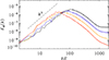 |
Fig. 1. Spectral energy of the Cartesian reference run R1. The magnetic spectra are displayed at |


Toward the end of the simulation, we notice that the inverse cascade stalls when ℓ0 ≈ 30, with almost no further transfer of energy toward the dipolar component. In the following sections, we examine the impact of the coordinate system, peak wavenumber position, aspect ratio, and boundary conditions to understand what is limiting the inverse cascade from transferring energy to larger-scale structures.
4.2. Different coordinate systems
To study the impact of the coordinate systems on the inverse cascade, we replicated run R1 in spherical coordinates using PENCIL CODE in run R2 (see Table 2) and in cubed-sphere coordinates using MATINS in run Rι5 (see Table 4). These two runs have an average value of Lu similar to that of run R1, both on the order of a few hundred. The crustal shell is in the range r/R = 0.9 − 1 for both runs. In run R2, we choose θ/π = 0.1 − 0.9 to avoid the axis singularity problem in 3D spherical coordinates, while ϕ/π = 0 − 1. By contrast, run Rι5 covers the full crustal shell and has θ/π = 0 − 1, and ϕ/π = 0 − 2.
The meridional slices of the Br(r, θ) component of the magnetic field for run R2 are illustrated in Figure 2 at three different times:  , 2 × 10⁻⁶, and 6 × 10⁻⁶ (from left to right). Initially, the magnetic spectrum predominantly features small-scale structures on the order of k0R ≈ 200 (at
  ). As the evolution processes, the emergence of large-scale structures from small-scale ones becomes increasingly apparent, ultimately resulting in magnetic field structures comparable in size to the NS crust. This growth in scale hints at why the inverse cascade concludes, which can be attributed to the extreme aspect ratio 𝒜 of the NS crust. The inverse cascade phenomenon observed in the magnetic field of run R2 is further corroborated by the magnetic energy spectra shown in Figure 3 at various times.
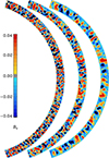 |
Fig. 2. Meridional slices of Br(r, θ) for run R2, with |


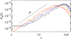 |
Fig. 3. Spectral energy of the spherical run R2. As in Figure 1, the magnetic spectra are shown at |

To verify if the same behavior occurs with cubed-sphere coordinates, we conducted simulations using MATINS. This test is also essential for determining if two different numerical codes yield similar results. As demonstrated previously using the PENCIL CODE, for the inverse cascade to occur, the initial magnetic spectrum should predominantly exhibit small-scale structures with ℓ0 ≈ 200. However, achieving the necessary resolution with MATINS is challenging because it is not parallelized, unlike the PENCIL CODE.
An alternative approach involves concentrating more structures exclusively in the radial direction. This initial magnetic field configuration can be conceptualized as a squashed magnetic field structure, achieved by selecting an ι value greater than one; see Eq. (16). The ι parameter is determined based on the results from run R1. During run R1, the initial value  decreased to
  . By this time, the radial scale has reduced to π/k ≈ 0.1, corresponding to the crustal thickness, and the inverse cascade concluded. This indicates that for the inverse cascade to remain active, ℓ must not fall significantly below the inverse aspect ratio ≳𝒜−1. To span a factor ℱ ≈ 200/30 in the inverse cascade during MATINS simulations with ℓmax = 80, where the affordable spherical degree at the peak is ℓ0afford ≈ 40, the radial scale must be reduced by a squashing factor ι. The value of ι can be computed using the following equation:
 (28)
(28)
For example, with ℓ0afford ≈ 40 in MATINS, an ι value of approximately 5 is required to accommodate ℓ0 ≈ 200.
Figure 4 presents the magnetic energy spectra for the Rι5 simulation at four different times: t0 = 0.0 (black), t1 = 0.005 (blue), t2 = 0.01 (yellow), and t3 = 0.02 Myr (red). The Ohmic diffusion timescale, defined as ξ2/η, is approximately 0.02 Myr. Similar to the Cartesian and spherical runs (R1 and R2) conducted with the PENCIL CODE, the magnetic field in run Rι5 exhibits an inverse cascade, featuring ascending ℓ3 spectra and demonstrating temporal decay that scales as ℓ3/2 on the cubed-sphere grid (not shown). Figure 5 shows meridional slices of the Br(r, θ) component of the magnetic field for run Rι5 at t = 0.0, 0.01 and, 0.02 Myr. The radial magnetic field structures are visibly squashed along the radial direction. Notably, the inverse cascade observed in MATINS is less pronounced than in the PENCIL CODE, as demonstrated in Figures 4 and 5. This discrepancy may be related to the ι parameter (Eq. (28)), which represents the squashing factor.
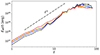 |
Fig. 4. Spectral energy of the cubed-sphere run Rι5 at t0 = 0.0 (black), t1 = 0.005 Myr (blue), t2 = 0.01 Myr (yellow), and t3 = 0.02 Myr (red). |
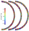 |
Fig. 5. Meridional slices of Br(r, θ) for run Rι5 at t = 0.0, 0.01 Myr and, 0.02 Myr (from left to right). |
The consistent behavior observed in run R1, run R2, and run Rι5, which utilize Cartesian, spherical, and cubed-sphere coordinates respectively, indicates that the choice of coordinate system is not critical as long as the initial conditions (and the correct aspect ratio) are nearly identical. Notably, despite the differing geometrical coordinates, all three models exhibit an inverse cascade limited to ℓ0 ≈ 30, with minimal energy transfer to the dipolar component.
4.3. Effects of peak position
In this section, we examine the effect of varying initial k0R values on the inverse cascade using MATINS simulations. In the first case, we set ι = 1 (see Equation (28)) for run Rι1, resulting in k0R = 40. In the second case, ι was increased to 10 for run Rι10, resulting in k0R = 400. These simulations were designed to test our interpretation of the squashed initial field configuration in MATINS and evaluate whether it yields the anticipated results.
Figure 6 presents the results for runs Rι1 (upper panel) and Rι10 (lower panel) at various stages of evolution. In run Rι1, no inverse cascade is observed, likely because the field structures are comparable in size to the crustal thickness. In contrast, run Rι10 exhibits a clear and more pronounced inverse cascade compared to run Rι5. These results suggest that the presence of small-scale initial spherical degrees is crucial for the inverse cascade to occur.
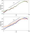 |
Fig. 6. Spectral magnetic energy for run Rι1 (upper panel) and run Rι10 (lower panel). As in Figure 4, the magnetic spectra are shown at t = 0.0 (black), 0.005 (blue), 0.01 (yellow), 0.02 (red), and 0.04 Myr (green). |
4.4. Aspect ratio
To study the impact of the aspect ratio on the inverse cascade, we conducted a replication of the reference run R1, and in this iteration, we adjusted solely the crust aspect ratio. On the one hand, in the new run R3 (see Table 2), we doubled the crustal thickness. Consequently, the crustal shell is now in the range r/R = 0.8 − 1, accounting for one-fifth of the entire NS cross-sectional area, as opposed to the previous one-tenth. On the other hand, in the new run R4, we also doubled the crustal thickness and, in addition, we reduced θ/π and ϕ/π from the range of 0 − 1 to 0 − 0.5. Therefore, the geometry of our domain now approaches a cubic configuration.
The magnetic energy spectra for runs R3 and R4 are depicted in the upper and lower panels of Figure 7, respectively. In this representation, magnetic spectra are plotted at  (black), 2 × 10⁻⁶ (blue), 6 × 10⁻⁶ (yellow), and 2 × 10⁻⁵ (red). Compared to the reference run R1 (Figure 1), R3 and R4 exhibit a more pronounced inverse cascading phenomenon with several distinct behaviors.
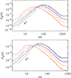 |
Fig. 7. Spectral energy of run R3 (upper panel) and run R4 (lower panel) in Cartesian coordinates, each characterized by different aspect ratios compared to the reference run R1. Data is shown at |

At  , the characteristic scale ℓ0 is approximately 20 for run R3 and 10 for run R4, whereas for run R1, ℓ0 ≈ 50 at the same time. Furthermore, at largest scale (ℓ ∼ 1), the spectral magnetic energy remains nearly constant in run R1, with EM(k)≈6 × 10⁻¹⁰. In contrast, runs R3 and R4 show significant energy accumulation in the dipolar component (ℓ ∼ 1), with EM(k)≈10−8 for run R3 and EM(k)≈10−6 for run R4.
Compared to run R3 and the reference run R1, run R4 demonstrates a more rapid inverse cascade, achieving a fully helical field state in a shorter time. For  , the peak of the magnetic energy spectrum,
  , in run R4 is steadily maintained throughout its evolution, indicating a convergence toward a maximally helical field. Meanwhile, the total magnetic energy continues to dissipate.
These differences relative to the reference run R1 are attributed to the aspect ratio, particularly in run R4, where the geometry approximates cubic symmetry, while run R3 involves only doubling the crustal thickness. Variations in crustal geometry significantly influence the inverse cascade, the efficiency of achieving a maximally helical field, and the formation of the large-scale magnetic field. The realistic extreme aspect ratio of the NS crust limits the inverse cascade, and the energy transfer toward the dipolar component.
At this stage, it is intriguing to explore whether a less extreme aspect ratio, as used in run R4, can reveal the presence or absence of an inverse cascade for a smaller initial ℓ0. To investigate this, we replicated run R4, adjusting ℓ0 from approximately 200 to 50 for run R5, as detailed in Table 2. The magnetic energy spectra for run R5 exhibit behavior similar to that of run R4, confirming the presence of an inverse cascade even with an initial peak wavenumber of ℓ0 ≈ 50. Notably, at  , the peak wavenumber for both runs R4 and R5 reaches ℓ0 ≈ 10, as shown in Table 2. As previously mentioned, this outcome is influenced by the crustal geometry used in both runs, which closely resembles a cubic configuration. We note that starting with ℓ0 ≈ 50 in a model replicating the reference run R1 does not result in an inverse cascade.
4.5. Periodic boundary conditions
In this section, we examine the impact of magnetic boundary conditions on our simulations. To do so, we replicate reference run R1, but modify the magnetic boundary conditions by replacing the perfect conductor and vertical field boundary conditions on the inner and outer radial boundaries, respectively, with periodic boundary conditions. In Table 2 it is labeled as run R6.
The magnetic spectrum of run R6 is illustrated in Figure 8 at various times. The magnetic field undergoes pronounced inverse cascading. However, unlike the reference run R1, run R6 exhibits energy transfer to low spherical degree (ℓ ∼ 1), with EM(k)≈2 × 10⁻⁹ compared to EM(k)≈6 × 10⁻¹⁰ in run R1 at  . This energy transfer is less efficient than in runs R3 and R4. On the other hand, the inverse cascade remains limited to ℓ0 ≈ 50, the same as in run R1 at
  . Consequently, adopting periodic boundary conditions does not explain the formation of the large-scale magnetic field in magnetars.
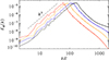 |
Fig. 8. Spectral energy of run R6 in Cartesian geometry, characterized using periodic boundary conditions compared to reference run R1. Data is shown at |

In contrast to the reference run R1, where the magnetic spectrum undergoes temporal decay, run R6 exhibits a stable value of  throughout its evolution. The energy spectrum of run R6 aligns with the characteristics of fully helical MHD spectra; see the end of Sect. 2.2 for details on a fully helical magnetic field and Figure 5 in Brandenburg (2020). Nonperiodic boundary conditions–such as potential, vertical, and perfect conductor boundaries–resulted in a partially helical field, explaining the decay in
  . In contrast, the periodic boundary conditions in run R6 facilitate the development of a fully helical magnetic field.
5. Discussion
Studying the inverse cascade in NS crusts presents a significant challenge, as it remains a relatively unexplored topic in the existing literature. A notable exception is the work of Brandenburg (2020), which employed local simulations of the Hall cascade and identified the occurrence of an inverse cascade. However, these simulations, restricted to a cubic domain, are not adequate for capturing the complex and realistic properties of the NS crust.
In contrast, Gourgouliatos et al. (2020) explored the possibility of an inverse cascade in the NS crust but found no evidence of its occurrence. While an increase in the dipole component of the magnetic field was observed, the hallmark feature of an inverse cascade–a shift in the energy spectrum peak from smaller to larger scales–was absent. In their setup, magnetic energy was initially concentrated in multipoles within the range ℓ = 10 − 20, with minimal or zero contributions from other multipoles. Mode coupling, driven by the nonuniformity of coefficients and Hall nonlinearity, redistributed energy to neighboring multipoles and resulted in a shallow energy spectrum dominated by the initial scales. Instead of a spectral peak shifting to larger scales, energy redistributed to multipoles that initially carried negligible magnetic energy, with no discernible evidence of an inverse cascade manifesting. Over time, smaller-scale structures dissipated as Hall drift became less efficient, shaping their final energy spectra. The lack of magnetic helicity measurements in their study left a critical gap in understanding–specifically, whether the absence of an inverse cascade was due to the lack of magnetic helicity or the initial dominance of structures at scales comparable to the NS crust.
Despite these efforts, several critical factors remained unaddressed within a single comprehensive setup. These include high resolution simulations capable of resolving small-scale structures while incorporating the correct aspect ratio, spherical geometry, an initial causal spectrum (Sect. 3.3) designed to better capture conditions conducive to an inverse cascade, appropriate boundary conditions, and the consideration of time-dependent magnetic diffusivity–an essential factor influenced by the cooling processes of NSs.
To address these gaps, our research undertook a comprehensive investigation to evaluate the efficacy of the inverse cascade in the NS crust. Our work also aimed to understand its potential role in explaining the origin of the large-scale dipolar field observed in magnetars–an intriguing question with significant implications. A crucial requirement for a strong inverse cascade to occur is the presence of an initial helical magnetic field (Brandenburg 2020). Nonhelical magnetic fields can also induce an inverse cascade via the Hall effect (Brandenburg 2023), but it is weaker. To produce an initially helical magnetic field, we developed a formalism for both Cartesian and spherical coordinates, allowing for systematic study using the PENCIL CODE and MATINS.
The slenderness of the NS crust adds complexity, necessitating initial peak wavenumbers from small-scale structures on the order of k0R ≈ 200 for the inverse cascade to occur. Resolving these scales requires high-resolution simulations, which is challenging. To overcome this, MATINS introduces additional wavenumbers in the radial direction, whereas the PENCIL CODE does not encounter this issue. MATINS lacks parallelization, making it less computationally powerful than the PENCIL CODE.
In our reference run R1, we constructed a model in Cartesian coordinates with an initial helical field dominated by small-scale structures, k0R ≈ 200, while maintaining the correct aspect ratio of the NS crust (see Sect. 4.1). This setup was designed to optimally observe the inverse cascade, as the peak wavenumber shifted towards larger-scale structures within the crust’s interior. However, the spectra revealed limitations: dissipation of the peak wavenumber (attributable to the use of nonperiodic boundary conditions that enforced a partially helical field), restriction of the cascade to k0R ≈ 30, and negligible energy transfer to the largest-scale structure (kR ≈ 1). To understand these phenomena, we explored the influence of geometrical coordinates, initial peak position, aspect ratio, and boundary conditions.
To explore the effects of geometry, we analyzed different coordinate systems in Sect. 4.2. Spherical coordinates were employed in the PENCIL CODE (run R2), with axis adjustments to avoid singularities, while cubed-sphere coordinates were used in MATINS (run Rι5), which inherently bypass this issue. Despite these differences, the results were consistent, demonstrating that the choice between Cartesian and spherical domains has no significant effect when initial conditions are nearly identical. This observation aligns with findings by Mitra et al. (2009). Additionally, in Sect. 4.3, we confirmed that small-scale initial spherical degrees (ℓ0 ≈ 200) are essential for the occurrence of the inverse cascade.
Expanding our analysis, we examined the role of aspect ratio by exploring various crustal domain configurations (Sect. 4.4). In the first case (Run R3), the crustal thickness was doubled. In the second case (Run R4), the crustal thickness was also doubled, but the domain in the angular directions θ/π and ϕ/π was halved, resulting in a nearly cubic geometry. Compared to the reference run R1, three main differences were observed: First, the peak wavenumber k0R continued shifting toward larger-scale structures and was no longer constrained to 30. Second, a significant transfer of energy toward the largest-scale structure (kR = 1) occurred. Third, the efficiency of achieving a fully helical field was more pronounced, especially in run R4, highlighting the impact of geometrical configuration on the development of a fully helical field, even under nonperiodic boundary conditions. These findings suggest that the thin-layer geometry of the NS crust hinders the inverse cascade, thereby limiting the formation of a large-scale magnetic field.
Building on these findings, we then investigated how different boundary conditions affect the spectral characteristics of the inverse cascade in Sect. 4.5. Our results indicated that, using periodic boundary conditions (run R6) rather than perfect conductor boundary conditions at the crust-core interface or potential and vertical field boundary conditions at the surface, resulted in  being approximately constant. Periodic boundary conditions produce a fully helical magnetic field (see Brandenburg 2020), unlike other boundary conditions, which result in a partially helical field (Brandenburg 2017). For a fully helical field, the constancy of the mean magnetic helicity density ensures that the spectral peak height
  remains unchanged as the typical length scale ξ increases and the mean magnetic energy density decreases (refer to the end of Sect. 2.2, for more details).
While periodic boundary conditions offer insights, they are not a realistic choice for studying the NS scenario. Similarly, using perfect conductor boundary conditions, which expel the field from the NS core, and vertical field or potential boundary conditions, which prevent current flow outside the star, do not fully capture the realistic conditions of magnetic field evolution in a NS crust. Carefully addressing boundary conditions is crucial for gaining a better understanding of the inverse cascade in NS crusts. Although this level of detail is beyond the scope of this paper and not feasible with the numerical tools currently available, it remains an important consideration for future studies.
In this study, we disregarded the exact temperature-dependent microphysics and the stratification within the interior of a NS crust, anticipating that these factors would not significantly impact our findings regarding the inverse cascade. The temperature-dependent microphysics is expected to reduce the magnetic diffusion parameter as the NS cools over time, leading to a higher Lundquist number (see Section 5.4 of Dehman et al. 2023b). Our simulations have partially reflected this through a time-dependent magnetic diffusivity, as shown in Eq. (26). Additionally, there is a radial dependence of Lu ∝ (neη)−1; see Eq. (11). Gourgouliatos et al. (2020) considered the case of moderate stratification with ne ∝ [1 − (r − R)/He]4 and He/R = 0.0463, and used η ∝ ne−2/3, so Lu ∝ ne−1/3 increased by a factor of about five from r/R = 1 down to 0.9. Using their approximation, Brandenburg (2020) found that Brms decays more slowly with depth, and ξ increased only ∝t1/3. Nevertheless, the relation between magnetic dissipation and magnetic field strength was found to be remarkably similar to the unstratified case. Furthermore, Cumming et al. (2004) demonstrated that at all depths, the transition from ohmic decay–dominated behavior to Hall-dominated behavior occurs at roughly the same time.
To ensure a Hall-dominant simulation and the occurrence of an inverse cascade, the Lundquist number must be significantly greater than one (Lu ≫ 1). We initialized our study with a Lundquist number on the order of a few hundred, simulating a magnetar-like scenario. Consequently, our Hall-dominant simulations are representative of magnetic field evolution in middle-aged magnetars. Since the aspect ratio limits the inverse cascade to field structures on the order of the crustal size, k0R ≈ 30, we expect that considering a density (or radius) dependent Lundquist number will not change this conclusion.
In light of these insights, it is essential to consider realistic NS parameters, particularly the crustal thickness and its correct aspect ratio, when investigating the inverse cascade within a NS crust. While the inverse cascade cannot account for the formation of the large-scale dipolar field in magnetars–where the dipolar component remains on the order of 1012 − 1013 G–it does occur within the crust’s interior at smaller scales. These findings have significant implications for the evolution of NS magnetic fields. Our study reveals a field configuration characterized by a weak, large-scale dipolar component (≈1012 − 1013 G), along with dominant small-scale magnetic fields (≈1014 − 1015 G). The inverse cascade mechanism plays a crucial role by transferring energy from turbulent small scales to larger scales, effectively reducing small-scale dissipation. This energy transfer shapes the field’s configuration and stability, influencing the crustal lattice dynamics and potentially impacting NS asteroseismology (Steiner & Watts 2009; Sotani et al. 2012; Neill et al. 2023), crustal failures (Perna & Pons 2011; Pons & Perna 2011; Dehman et al. 2020), plastic flow within the star’s interior (Lander et al. 2015; Lander & Gourgouliatos 2019; Gourgouliatos & Lander 2021), and may explain key observational properties of low-field magnetars and CCOs, which exhibit these characteristic magnetic features.
In summary, incorporating a helical magnetic field into the evolution of a NS’s crust favors the occurrence of an inverse cascade, which reshapes the magnetic field over time. This process influences key mechanisms that determine the star’s physical properties and observational characteristics.
Data availability
The source code used for the simulations of this study, the PENCIL CODE (Pencil Code Collaboration 2021), is freely available on https://github.com/pencil-code/. The simulation setups and corresponding input and reduced out data are freely available on https://doi.org/10.5281/zenodo.14513354; see also http://norlx65.nordita.org/~brandenb/projects/Reality-InvCasc-NS for easier access of the same data.
The public routines implemented in MATINS are available at http://www.ioffe.ru/astro/conduct/. For details, see Potekhin et al. (2015).
The plotted energy spectrum (Eq. (8)) in MATINS is a 2D spectrum decomposed into spherical harmonics along θ and ϕ coordinates.
NSs consist of degenerate matter, typically characterized by temperatures lower than the Fermi temperature for their entire existence. In this specific temperature range, quantum effects, as dictated by Fermi statistics, overwhelmingly dominate over thermal effects. Therefore, the EoS for NSs can be effectively approximated as that of zero temperature, allowing us to largely ignore thermal contributions for most of their lifespan.
Acknowledgments
We thank the anonymous referee for their useful suggestions. We acknowledge the inspiring discussions with participants in the programs “Turbulence in Astrophysical Environments” at the Kavli Institute for Theoretical Physics, Santa Barbara (NSF PHY-2309135), and the Munich Institute for Astro-, Particle and BioPhysics (MIAPbP), which is funded by the Deutsche Forschungsgemeinschaft (DFG, German Research Foundation) under Germany’s Excellence Strategy – EXC-2094 – 390783311, as well as with Jose A. Pons. We also acknowledge the visiting PhD fellow program at Nordita, which partially funded this research. This research was supported in part by the Swedish Research Council (Vetenskapsrådet) under Grant No. 2019-04234, the National Science Foundation under Grant No. AST-2307698 and the NASA ATP Award 80NSSC22K0825. We also acknowledge funding from the Conselleria d’Educació, Cultura, Universitats i Ocupació de the Generalitat Valenciana through grants CIPROM/2022/13 and ASFAE/2022/026 (with funding from NextGenerationEU PRTR-C17.I1), as well as the AEI grant PID2021-127495NB-I00 funded by MCIN/AEI/10.13039/501100011033. We acknowledge the allocation of computing resources provided by the Swedish National Allocations Committee at the Center for Parallel Computers at the Royal Institute of Technology in Stockholm.
References
- Akgün, T., Cerdá-Durán, P., Miralles, J. A., & Pons, J. A. 2018, MNRAS, 481, 5331 [CrossRef] [Google Scholar]
- Aloy, M. Á., & Obergaulinger, M. 2021, MNRAS, 500, 4365 [Google Scholar]
- Ascenzi, S., Viganò, D., Dehman, C., et al. 2024, MNRAS, 533, 201 [NASA ADS] [CrossRef] [Google Scholar]
- Balbus, S. A., & Hawley, J. F. 1991, ApJ, 376, 214 [Google Scholar]
- Brandenburg, A. 2017, A&A, 598, A117 [NASA ADS] [CrossRef] [EDP Sciences] [Google Scholar]
- Brandenburg, A. 2020, ApJ, 901, 18 [NASA ADS] [CrossRef] [Google Scholar]
- Brandenburg, A. 2023, J. Plasma Phys., 89, 175890101 [NASA ADS] [CrossRef] [Google Scholar]
- Brandenburg, A., & Boldyrev, S. 2020, ApJ, 892, 80 [NASA ADS] [CrossRef] [Google Scholar]
- Brandenburg, A., & Kahniashvili, T. 2017, Phys. Rev. Lett., 118, 055102 [NASA ADS] [CrossRef] [Google Scholar]
- Brandenburg, A., & Subramanian, K. 2005, Phys. Rep., 417, 1 [NASA ADS] [CrossRef] [Google Scholar]
- Brandenburg, A., Kahniashvili, T., & Tevzadze, A. G. 2015, Phys. Rev. Lett., 114, 075001 [NASA ADS] [CrossRef] [Google Scholar]
- Brandenburg, A., Kamada, K., Mukaida, K., Schmitz, K., & Schober, J. 2023a, Phys. Rev. D, 108, 063529 [NASA ADS] [CrossRef] [Google Scholar]
- Brandenburg, A., Kamada, K., & Schober, J. 2023b, Phys. Rev. Res., 5, L022028 [CrossRef] [Google Scholar]
- Chandrasekhar, S. 1981, Hydrodynamic and Hydromagnetic Stability, Dover Books on Physics Series (Dover Publications) [Google Scholar]
- Chandrasekhar, S., & Kendall, P. C. 1957, ApJ, 126, 457 [Google Scholar]
- Cho, J. 2011, Phys. Rev. Lett., 106, 191104 [NASA ADS] [CrossRef] [Google Scholar]
- Cumming, A., Arras, P., & Zweibel, E. 2004, ApJ, 609, 999 [NASA ADS] [CrossRef] [Google Scholar]
- Dehman, C., & Pons, J. A. 2024, ArXiv e-prints [arXiv:2408.05281] [Google Scholar]
- Dehman, C., Viganò, D., Rea, N., et al. 2020, ApJ, 902, L32 [NASA ADS] [CrossRef] [Google Scholar]
- Dehman, C., Viganò, D., Ascenzi, S., Pons, J. A., & Rea, N. 2023a, MNRAS, 523, 5198 [NASA ADS] [CrossRef] [Google Scholar]
- Dehman, C., Viganò, D., Pons, J. A., & Rea, N. 2023b, MNRAS, 518, 1222 [Google Scholar]
- Durrer, R., & Caprini, C. 2003, JCAP, 2003, 010 [CrossRef] [Google Scholar]
- Esposito, P., Rea, N., & Israel, G. L. 2021, Astrophys. Space Sci. Lib., 461, 97 [NASA ADS] [CrossRef] [Google Scholar]
- Frisch, U., Pouquet, A., Leorat, J., & Mazure, A. 1975, J. Fluid Mech., 68, 769 [NASA ADS] [CrossRef] [Google Scholar]
- Geppert, U., & Wiebicke, H.-J. 1991, A&AS, 87, 217 [NASA ADS] [Google Scholar]
- Goldreich, P., & Reisenegger, A. 1992, ApJ, 395, 250 [NASA ADS] [CrossRef] [Google Scholar]
- Gourgouliatos, K. N., & Lander, S. K. 2021, MNRAS, 506, 3578 [NASA ADS] [CrossRef] [Google Scholar]
- Gourgouliatos, K. N., Hollerbach, R., & Igoshev, A. P. 2020, MNRAS, 495, 1692 [Google Scholar]
- Igoshev, A. P., Popov, S. B., & Hollerbach, R. 2021, Universe, 7, 351 [NASA ADS] [CrossRef] [Google Scholar]
- Krause, F., & Rädler, K.-H. 1980, Mean-Field Magnetohydrodynamics and Dynamo Theory (Oxford: Pergamon Press) [Google Scholar]
- Lander, S. K., Andersson, N., Antonopoulou, D., & Watts, A. L. 2015, MNRAS, 449, 2047 [NASA ADS] [CrossRef] [Google Scholar]
- Lander, S. K., & Gourgouliatos, K. N. 2019, MNRAS, 486, 4130 [NASA ADS] [CrossRef] [Google Scholar]
- Masada, Y., Kotake, K., Takiwaki, T., & Yamamoto, N. 2018, Phys. Rev. D, 98, 083018 [NASA ADS] [CrossRef] [Google Scholar]
- Mitra, D., Tavakol, R., Brandenburg, A., & Moss, D. 2009, ApJ, 697, 923 [NASA ADS] [CrossRef] [Google Scholar]
- Moffatt, H. K. 1978, Magnetic Field Generation in Electrically Conducting Fluids (Cambridge: Cambridge University Press) [Google Scholar]
- Neill, D., Preston, R., Newton, W. G., & Tsang, D. 2023, Phys. Rev. Lett., 130, 112701 [NASA ADS] [CrossRef] [Google Scholar]
- Obergaulinger, M., Janka, H. T., & Aloy, M. A. 2014, MNRAS, 445, 3169 [CrossRef] [Google Scholar]
- Oppenheimer, J. R., & Volkoff, G. M. 1939, Phys. Rev., 55, 374 [NASA ADS] [CrossRef] [Google Scholar]
- Ostriker, J. P., & Gunn, J. E. 1969, ApJ, 157, 1395 [Google Scholar]
- Pencil Code Collaboration (Brandenburg, A., et al.) 2021, JOSS, 6, 2807 [CrossRef] [Google Scholar]
- Perna, R., & Pons, J. A. 2011, ApJ, 727, L51 [NASA ADS] [CrossRef] [Google Scholar]
- Pons, J. A., & Perna, R. 2011, ApJ, 741, 123 [NASA ADS] [CrossRef] [Google Scholar]
- Potekhin, A. Y., Pons, J. A., & Page, D. 2015, Space Sci. Rev., 191, 239 [Google Scholar]
- Raynaud, R., Guilet, J., Janka, H.-T., & Gastine, T. 2020, Sci. Adv., 6, eaay2732 [NASA ADS] [CrossRef] [Google Scholar]
- Reboul-Salze, A., Guilet, J., Raynaud, R., & Bugli, M. 2021, A&A, 645, A109 [NASA ADS] [CrossRef] [EDP Sciences] [Google Scholar]
- Rogachevskii, I., Ruchayskiy, O., Boyarsky, A., et al. 2017, ApJ, 846, 153 [NASA ADS] [CrossRef] [Google Scholar]
- Ronchi, C., Iacono, R., & Paolucci, P. 1996, J. Comput. Phys., 124, 93 [NASA ADS] [CrossRef] [Google Scholar]
- Sarin, N., Brandenburg, A., & Haskell, B. 2023, ApJ, 952, L21 [NASA ADS] [CrossRef] [Google Scholar]
- Schober, J., Rogachevskii, I., Brandenburg, A., et al. 2018, ApJ, 858, 124 [NASA ADS] [CrossRef] [Google Scholar]
- Sigl, G., & Leite, N. 2016, JCAP, 2016, 025 [Google Scholar]
- Sotani, H., Nakazato, K., Iida, K., & Oyamatsu, K. 2012, Phys. Rev. Lett., 108, 201101 [NASA ADS] [CrossRef] [Google Scholar]
- Steiner, A. W., & Watts, A. L. 2009, Phys. Rev. Lett., 103, 181101 [NASA ADS] [CrossRef] [Google Scholar]
- Thompson, C., & Duncan, R. C. 1995, MNRAS, 275, 255 [Google Scholar]
- Turolla, R., Zane, S., & Watts, A. L. 2015, Rep. Progr. Phys., 78, 116901 [Google Scholar]
- Urbán, J. F., Stefanou, P., Dehman, C., & Pons, J. A. 2023, MNRAS, 524, 32 [CrossRef] [Google Scholar]
- Wareing, C. J., & Hollerbach, R. 2009, A&A, 508, L39 [NASA ADS] [CrossRef] [EDP Sciences] [Google Scholar]
- Wareing, C. J., & Hollerbach, R. 2010, J. Plasma Phys., 76, 117 [NASA ADS] [CrossRef] [Google Scholar]
Appendix A: Magnetic formalism in 3D spherical coordinates
In spherical coordinates, various formalism can be used to describe the magnetic field. In this context, we present the most common notations found in the literature. For any three-dimensional solenoidal vector field B, representing the magnetic field, we can always introduce the vector potential A such that
 (A.1)
(A.1)
The magnetic field B can be expressed using the poloidal Φ(x) and the toroidal Ψ(x) scalar functions, based on the formalism of Chandrasekhar (1981):
 (A.2)
(A.2)
Using the notation of Krause & Rädler (1980) and Geppert & Wiebicke (1991), the two scalar functions can be expanded in a series of spherical harmonics:
 (A.3)
(A.3)
where ℓ = 1, …, ℓmax is the degree and m = −ℓ,…,ℓ the order of the multipole.
The three components of the vector potential A in spherical coordinates are obtained by combining the poloidal and toroidal components:
 (A.4)
(A.4)
The three components of the magnetic field B in the Newtonian limit are given by:
 (A.5)
(A.5)
Here, Φ′ℓm = ∂Φℓm/∂r, ignoring relativistic corrections. For the complete form, including relativistic corrections, refer to Dehman et al. (2023b). Using Equation (A.4) and Equation (A.5), one can derive the expressions for the spectral magnetic helicity Eq. (7), the spectral magnetic energy Eq. (8), and the spectral realizability condition Eq. (9).
All Tables
Spectrum of the magnetic vector potential A and the magnetic field B for k ≪ k0, depicting the ascending spectra.
Summary of MATINS simulations on a cubed-sphere grid representing a crustal shell.
All Figures
|
Fig. 1. Spectral energy of the Cartesian reference run R1. The magnetic spectra are displayed at |
| In the text | |
|
Fig. 2. Meridional slices of Br(r, θ) for run R2, with |
| In the text | |
|
Fig. 3. Spectral energy of the spherical run R2. As in Figure 1, the magnetic spectra are shown at |
| In the text | |
|
Fig. 4. Spectral energy of the cubed-sphere run Rι5 at t0 = 0.0 (black), t1 = 0.005 Myr (blue), t2 = 0.01 Myr (yellow), and t3 = 0.02 Myr (red). |
| In the text | |
|
Fig. 5. Meridional slices of Br(r, θ) for run Rι5 at t = 0.0, 0.01 Myr and, 0.02 Myr (from left to right). |
| In the text | |
|
Fig. 6. Spectral magnetic energy for run Rι1 (upper panel) and run Rι10 (lower panel). As in Figure 4, the magnetic spectra are shown at t = 0.0 (black), 0.005 (blue), 0.01 (yellow), 0.02 (red), and 0.04 Myr (green). |
| In the text | |
|
Fig. 7. Spectral energy of run R3 (upper panel) and run R4 (lower panel) in Cartesian coordinates, each characterized by different aspect ratios compared to the reference run R1. Data is shown at |
| In the text | |
|
Fig. 8. Spectral energy of run R6 in Cartesian geometry, characterized using periodic boundary conditions compared to reference run R1. Data is shown at |
| In the text | |
Current usage metrics show cumulative count of Article Views (full-text article views including HTML views, PDF and ePub downloads, according to the available data) and Abstracts Views on Vision4Press platform.
Data correspond to usage on the plateform after 2015. The current usage metrics is available 48-96 hours after online publication and is updated daily on week days.
Initial download of the metrics may take a while.