| Issue |
A&A
Volume 644, December 2020
|
|
|---|---|---|
| Article Number | A166 | |
| Number of page(s) | 14 | |
| Section | Stellar structure and evolution | |
| DOI | https://doi.org/10.1051/0004-6361/202038775 | |
| Published online | 16 December 2020 | |
The RGB tip of galactic globular clusters and the revision of the axion-electron coupling bound
1
INAF, Osservatorio d’Abruzzo, Via M. Maggini, 64100 Teramo, Italy
e-mail: This email address is being protected from spambots. You need JavaScript enabled to view it.
2
INFN, Laboratori Nazionali del Gran Sasso, Assergi, Italy
3
Dipartimento di Fisica e Astronomia, Università di Bologna, Via Gobetti 93/2, 40129 Bologna, Italy
4
INAF, Osservatorio di Astrofisica e Scienza dello Spazio di Bologna, Via Gobetti 93/3, 40129 Bologna, Italy
5
Departamento de Fisíca Teoríca y del Cosmos, Universidad de Granada, 18071 Granada, Spain
6
Physical Sciences, Barry University, 11300 NE 2nd Ave., Miami Shores 33161, USA
7
Dipartemento Interateneo di Fisica “Michelangelo Merlin”, Via Amendola 173, 70126 Bari, Italy
8
INFN, Sezione di Bari, Via Orabona 4, 70126 Bari, Italy
Received:
27
June
2020
Accepted:
6
October
2020
Abstract
Context. The production of neutrinos by plasma oscillations is the most important energy sink process operating in the degenerate core of low-mass red giant stars. This process counterbalances the release of energy induced by nuclear reactions and gravitational contraction, and determines the luminosity attained by a star at the moment of the He ignition. This occurrence coincides with the tip of the red giant branch (RGB), whose luminosity is extensively used as a calibrated standard candle in several cosmological studies.
Aims. We aim to investigate the possible activation of additional energy sink mechanisms, as predicted by many extensions of the so-called Standard Model. In particular, our objective is to test the possible production of axions or axion-like particles, mainly through their coupling with electrons.
Methods. By combining Hubble Space Telescope and ground-based optical and near-infrared photometric samples, we derived the RGB tip absolute magnitude of 22 galactic globular clusters (GGCs). The effects of varying the distance and the metallicity scales were also investigated. Then we compared the observed tip luminosities with those predicted by state-of-the-art stellar models that include the energy loss due to the axion production in the degenerate core of red giant stars.
Results. We find that theoretical predictions including only the energy loss by plasma neutrinos are, in general, in good agreement with the observed tip bolometric magnitudes, even though the latter are ∼0.04 mag brighter on average. This small shift may be the result of systematic errors affecting the evaluation of the RGB tip bolometric magnitudes, or, alternatively, it could be ascribed to an axion-electron coupling causing a non-negligible thermal production of axions. In order to estimate the strength of this possible axion sink, we performed a cumulative likelihood analysis using the RGB tips of the whole set of 22 GGCs. All the possible sources of uncertainties affecting both the measured bolometric magnitudes and the corresponding theoretical predictions were carefully considered. As a result, we find that the value of the axion-electron coupling parameter that maximizes the likelihood probability is gae/10−13 ∼ 0.60−0.58+0.32. This hint is valid, however, if the dominant energy sinks operating in the core of red giant stars are standard neutrinos and axions coupled with electrons. Any additional energy-loss process, not included in the stellar models, would reduce such a hint. Nevertheless, we find that values gae/10−13 > 1.48 can be excluded with 95% confidence.
Conclusions. The new bound we find represents the most stringent constraint for the axion-electron coupling available so far. The new scenario that emerges after this work represents a greater challenge for future experimental axion searches. In particular, we can exclude that the recent signal seen by the XENON1T experiment was due to solar axions.
Key words: elementary particles / stars: low-mass / globular clusters: general / Hertzsprung-Russell / C–M diagrams
© ESO 2020
1. Introduction
The observed properties of stars compared to model predictions have often been used to constrain various physical processes occurring in stellar interiors. In particular, the brightest stars on the red giant branch (RGB) of a globular cluster may probe some processes responsible for the energy generation, such as nuclear reactions, as well as the efficiency of energy sinks, the most important of which is the plasma neutrino emission. Indeed, in the core of these low-mass stars, which are close to the He ignition, the temperature reaches ∼100 MK, while the central density is ∼106 g cm−3. According to the Standard Model, in this condition free electrons are highly degenerate and neutrinos are efficiently produced by plasma oscillations. Once produced, neutrinos escape from the stellar core, a process that subtracts the thermal energy spent for their production. On the other hand, degenerate electrons are excellent heat conductors and, in turn, they allow an efficient redistribution of the thermal energy. In addition, the high pressure of degenerate electrons hampers the core contraction and the consequent release of gravitational energy. As a result of the combined effects of neutrino production and electron degeneracy, the maximum temperature moves outward, to a layer placed approximately 0.2 M⊙ from the center, and the He ignition is delayed. In this framework, the luminosity of the RGB tip, which is the luminosity of a star at the off-center He ignition, is determined by the efficiency of these physical processes.
Although the scenario we describe here is widely accepted, additional energy sink processes, as predicted by the most popular extensions of the Standard Model, may greatly modify our understanding of the RGB evolution, and, in particular, they may affect the theoretical predictions of the RGB tip luminosity. Since the RGB tip luminosity is also considered a reliable standard candle, often used in cosmological studies (see, e.g., Freedman et al. 2020), it is important to investigate the possible impact of these additional energy-loss processes. Among them, the most appealing is probably the production of axions, or, more generally, of axion-like particles (ALPs). The existence of axions, which are small and weak interactive pseudo-scalar particles, was firstly proposed more than 40 years ago to solve the so-called strong CP problem, that is, the lack of evidence for a violation of the charge-parity symmetry by strong interactions (Peccei & Quinn 1977; Weinberg 1978; Wilczek 1978). Furthermore, ALPs also emerge as pseudo-Nambu-Goldstone bosons of spontaneously broken global symmetries in high-energy extensions of the Standard Model.
Like plasma-neutrinos, axions or ALPs may be produced in the core of an RGB star by thermal processes, thus modifying the internal energy budget. The general rule is well known (Raffelt & Weiss 1995): the larger the production rate of weak interactive particles produced by a thermal process, the brighter the tip of the RGB. For this reason, the RGB tip luminosity can be used to constrain the properties of neutrinos and other weak interactive slim particles (WISPs). In the case of axions, Bremsstrahlung should be the most efficient production mechanism in RGB stars, while other processes, like Primakoff and Compton, are suppressed because of the high electron degeneracy1.
In a previous attempt, Viaux et al. (2013a) made use of I-band photometric data of NGC 5904 (M5), a well-studied globular cluster of the Milky Way, to derive an upper bound for the strength of the axion-electron coupling (gae). They found gae < 4.3 × 10⁻¹³ (95% C.L.). For this paper, we attempted to improve this constraint. Two are the major sources of uncertainty in the evaluation of the RGB tip luminosity: the bolometric corrections and the cluster distance. In addition to that, since the evolutionary timescale is rather short for stars in the brightest portion of the RGB, only few of them are usually observed within two or three magnitudes of the RGB tip. This occurrence hampers the clear identification of the RGB tip. In order to reduce this uncertainty, we extended the M5 constraint to other clusters. First of all, we considered V and I photometries of other two well-studied clusters, NCG 362 and NGC 104 (47 Tuc). In order to collect large and more complete samples of RGB stars, we combined catalogs of high spatial resolution Hubble Space Telescope (HST) images of the most crowded central regions with ground based observations of the external portions of the cluster fields. In addition, NGC 362 and NGC 104 are the only two galactic globular clusters (GGCs) for which a reliable distance can be estimated from the parallaxes reported in the latest Gaia Data Release 2 (Chen et al. 2018). Then, we extended our analysis to a sample of 22 GCs, for which near-infrared (near-IR) photometries are available following a wide observational campaign performed by Ferraro et al. (2000), Sollima et al. (2004), and Valenti et al. (2004a,b). The availability of JHK observations presents several advantages. Indeed, the brightest RGB stars are rather cool objects, and their spectral energy distribution is dominated by near-IR light. For this reason, near-IR bolometric corrections of RGB stars are more reliable than that required at shorter wavelengths, allowing a more reliable derivation of the bolometric magnitudes (see. e.g., Buzzoni et al. 2010). In addition, some of the brightest RGB stars are long period variables, whose amplitude may be quite large in the optical spectral range, while it is much smaller in the near-IR (Kiss & Bedding 2003).
The models used to estimate the RGB tip luminosity of GGCs are presented in Sect. 2, while the adopted photometric samples and the derivation of the absolute bolometric magnitude of the RGB tip are described in Sect. 3. The statistical analysis and its results are discussed in Sect. 4. A summary and conclusions follow.
2. Theoretical recipes
2.1. The RGB tip luminosity from stellar models
The stellar models we use in the following analysis were computed by means of the Full Network Stellar evolution code (FuNS). This code has been extensively used to calculate models of stars of any mass and chemical composition and the related nucleosynthesis. We recently included the terms that account for the energy loss caused by an axion production possibly induced by various thermal processes in the energy conservation equation, in particular, Primakoff, Bremsstrahlung, e+e− pair annihilation, and Compton scattering on electrons or nuclei. The current version of the FuNS code and the relevant input physics are described in Straniero et al. (2019)2. It also contains a detailed description of the algorithms we use to calculate the axion energy-loss rates3. Here, we summarize the most important input physics adopted in the present work.
In general, the convective boundaries are fixed according to the Ledoux criterion. No convective overshoot is applied. In the convective zones, the temperature gradient is computed according to the mixing-length theory, as described in Cox & Giuli (1968). The mixing length parameter, α = Λ/HP = 1.82, was calibrated so as to reproduce the solar radius (Piersanti et al. 2007). The FuNS code may also account for stellar rotation (Piersanti et al. 2013) and microscopic diffusion (Straniero et al. 1997 and Piersanti et al. 2007), but these processes are not included in the present stellar models.
The FuNS has been optimized to handle large nuclear networks, such as those required to follow the neutron-capture nucleosynthesis in AGB stars (see Straniero et al. 2006). For the purpose of the present work, we considered 19 reactions for the H burning, those describing a full pp-chain and CNO-cycle, and an α-chain for the He burning. All the stable isotopes of H, He, Li, Be, C, N, O, plus 20Ne, are explicitly included in the nuclear network. The reaction rates are from version 6 of the STARLIB database (Sallaska et al. 2013). We note that most of the H and He burning reaction rates in this database are based on available experimental data. Rates of reactions for which no experimental information exists, or extrapolation to low/high temperatures are required, were obtained by means of statistical (Hauser–Feshbach) models of nuclear reactions (TALYS code; Goriely et al. 2008). The luminosity of the RGB tip is particularly sensitive to the adopted rates of the 14N(p, γ)15O and the triple-α reactions. The first reaction is the bottleneck of the CNO cycle, and, in turn, it determines the rate of growth of the core mass during the RGB phase. This reaction has been the object of an intense experimental campaign performed by the LUNA collaboration down to a center-of-mass energy of 70 keV, which corresponds to the Gamov peak for the typical temperature of the H-burning shell in evolved RGB stars (Formicola et al. 2004; Imbriani et al. 2004; Lemut et al. 2006). Our knowledge of this reaction is illustrated in Fig. 1, where the rate reported in the STARLIB repository (Sallaska et al. 2013), is compared to those reported in Adelberger et al. (2011) and in the NACREII repository (Xu et al. 2013). We note that in the temperature range of 20–100 MK, the differences are always smaller than 10%. On the other hand, the triple-α reaction determines the He ignition, and, in turn, it fixes the brightest point attained by an RGB star. The most recent experimental investigation of this reaction was reported by Fynbo et al. (2005). Nevertheless, the widely adopted reaction rates, such as those reported in STARLIB or REACLIB (Cyburt et al. 2010), are all based on the NACRE rate (Angulo et al. 1999). In any case, in the temperature range of 100 to 300 MK, the differences between the Fynbo et al. (2005) and the NACRE rates are less than the quoted 20% error. Finally, screening corrections are computed according to Dewitt et al. (1973), Graboske et al. (1973), and Itoh et al. (1979), for weak, intermediate, and strong ion coupling, respectively. The importance of the nuclear screening in the computation of RGB models is discussed in Sect. 2.4.
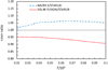 |
Fig. 1. 14N(p, γ)15O reaction rates suggested by the collaborations NACRE II and Solar Fusion are compared to the rate reported in the STARLIB repository. |
Concerning the neutrino-energy-loss rates, the most important contribution in RGB stars is due to plasma neutrinos (Haft et al. 1994). FuNS also includes the energy losses due to photo and pair neutrinos (Itoh et al. 1996), Bremsstrahlung neutrinos (Dicus et al. 1976), and recombination neutrinos (Beaudet et al. 1967).
Radiative opacities are computed according to Lederer & Aringer (2009), for log T ≤ 4, and to Iglesias & Rogers (1996), at larger temperature, while electron conductivity are from Potekhin et al. (1999) and Potekhin (1999).
The equation of state (EoS) is computed according to Rogers et al. (1996), for log T < 6.5, and to Straniero (1988) and Prada Moroni & Straniero (2002), at larger temperature (see Sect. 2.3 for further details).
The Henyey method employed in the FuNS to solve the stellar structure equations is a first-order implicit method, and the accuracy of the solutions depends on the assumed mass and time resolutions. We employed an adaptive algorithm to select the grid of mass shells and the time steps. In particular, the variations between adjacent mesh points of luminosity, pressure, temperature, mass, and radius should be:
 (1)
(1)
where A is one of L, P, T, M, or R. In the present work, we used δ = 0.05 everywhere, except for the shells located around some critical points, such as the boundaries of the convective zones, for which we used δ = 0.005. Similarly, the algorithm that we used to fix the time steps limits the variations of physical and chemical variables. Typically, when models climb the RGB, the total number of mesh points is about 1500, while the time step decreases from Δt ∼ 3 × 10⁴ yr, at log L/L⊙ = 2.1, down to Δt ≤ 103 yr, for log L/L⊙ > 3. Finally, the external boundary conditions were fixed according to a scaled solar T(τ) relation (Krishna Swamy 1966).
The set of stellar models on which our analysis is based is illustrated in Table 1. These models share the age at the RGB tip, namely ∼13 Gyr, and the initial He mass fraction, namely Y = 0.25. The metallicity (Z) and the corresponding [M/H] are listed in Cols. 1 and 2, respectively, while the resulting bolometric magnitudes at the RGB tip are reported in Col. 4. Variations of the cluster parameters, that is, age, Y, and Z as well as the theoretical uncertainties are discussed in Sects. 3.5 and 2.3, respectively.
Theoretical predictions of the tip bolometric magnitudes for globular cluster models with age = 13 Gyr and Y = 0.25.
2.2. Axions by RGB stars
In stellar interiors, axions can be produced through their interactions with standard model particles, mainly with photons and electrons, and, to a lesser extent, with nucleons. The Primakoff process, that is, the conversion of a photon into an axion in the electromagnetic field of an ion, γ + Ze → a + Ze, is the major consequence of the coupling with photons. The energy-loss rate due to this process depends on the square of gaγ, a quantity representing the strength of the axion-photon coupling. This rate increases as T4, but it is suppressed at the density of the RGB core due to the electron screening that reduces the effective charge of the nuclei. By adopting the present upper bound for the axion-photon coupling, that is, gaγ = 6 × 10⁻¹¹ GeV−1 (Ayala et al. 2014; Anastassopoulos et al. 2017), we found that the Primakoff process alone would produce a maximum decrease of the tip bolometric magnitude by ∼0.05 mag. Regarding the coupling with electrons, the most important axion sources at T ∼ 108 K are the Compton scattering, γ + e → γ + e + a, and the Bremsstrahlung, e + Ze → e + Ze + a. As noted by Raffelt & Weiss (1995), owing to the large electron degeneracy, which develops in the core of a red giant star, the Compton process is suppressed due to the Pauli blocking. On the contrary, the Bremsstrahlung process may induce a sizable axion production. The energy-loss rate due to Bremsstrahlung axion scales as the square of gae, a quantity representing the strength of the axion-electron coupling.
In Fig. 2, we compare the plasma-neutrino luminosity with those expected from axion emission due to Compton and Bremsstrahlung. This figure refers to a model with M = 0.82 M⊙, Y = 0.25, and Z = 0.001, and an axion-electron coupling gae = 10−13. Almost the whole RGB evolution is shown, from log L/L⊙ = 1 to the tip. After the RGB bump, which corresponds to the double luminosity inversion occurring at log L/L⊙ ∼ 2, the neutrino emission becomes the dominant energy-loss process. Close to the RGB tip (just before the He ignition) the neutrino luminosity is about five times the axion luminosity. On the other hand, Bremsstrahlung is the leading axion-emission process in RGB stars, more than one order of magnitude brighter than Compton. Finally, Fig. 3 shows the energy-loss rates within the core just before the He ignition. We note that while neutrinos are mainly emitted near the center, where the density is higher, the axion energy loss peaks at ∼0.2 M⊙ out of the center, where the temperature attains its maximum.
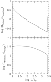 |
Fig. 2. Upper panel: evolution of ratio between axion and neutrino luminosites, from the base of the RGB (log L/L⊙ = 1) to the RGB tip, for a model with M = 0.82 M⊙, Y = 0.25, and Z = 0.001. Only the coupling with electrons has been switched on (g13 = 1). Lower panel: evolution of the ratio between Bremsstrahlung and Compton axion luminosities. |
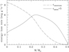 |
Fig. 3. Neutrinos and axions energy-loss rate within the core of a RGB model close to the RGB tip (just before the He ignition). Model parameters as in Fig. 2. |
The variations of the tip bolometric magnitudes as a function of gae are reported in Table 1 for models with different initial metallicities (see also, Fig. 4). Here, g13 = gae × 1013. The corresponding reductions of the tip bolometric magnitudes with respect to models without axions are reported in the last column of Table 1. We note that the more metal poor models show a higher sensitivity to the axion-electron coupling. As a whole, a g13 = 6 would imply ∼1 mag brighter bolometric magnitude, a value that is evidently incompatible with the observed RGB tip luminosity. A more stringent constraint can be obtained by means of a detailed evaluation of the error budget.
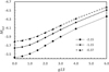 |
Fig. 4. Relation Mbol at the RGB tip versus g13 for 3 different metallicities ([M/H]). |
2.3. Theoretical uncertainty
For the purpose of the present work, we carried out a sensitivity study, with the aim of assigning a sort of theoretical error to the model prediction of the RGB tip luminosity. There are many examples of this kind of study in the extant literature (Viaux et al. 2013b; Valle et al. 2013; Serenelli et al. 2017). In these papers, the reader can find exhaustive illustrations of the various uncertainties affecting the relevant input physics. We do not repeat this discussion here. The uncertainties we adopted are listed in Table 2. From Col. 1 to Col. 4, we report: (1) the model inputs; (2) the reference for the preferred values; (3) the assumed 1σ errors; (4) the variations of the RGB tip bolometric magnitudes implied by the variation of each input physics within the assumed error bar (full width). The quantities ΔMbol reported in the last column represent the sensitivity of the predicted tip bolometric magnitude to the various model inputs. We note that the relationship between tip luminosity and model input is often nonlinear, so the uncertainty may be not perfectly symmetric around the central Mbol value. For this reason, in the last column of Table 2 we report the full-width variation rather than the half-width one. In any case, a rough estimation of the cumulative theoretical error may be obtained by summing the (average) half-width variations in quadrature, that is, ΔMbol/2. The result is σtheo ∼ 0.04. On the other hand, a more accurate estimation of this error can be obtained by means of a Monte Carlo propagation method. In practice, we assumed that each one of the listed model inputs (except for the microscopic diffusion and EoS) may vary according to a normal error distribution function. This assumption, which is appropriate when the uncertainty represents statistical fluctuations of experimental measurements, is certainly not strictly appropriate when the model input has been obtained through a theoretical calculation. Nevertheless, this is still a reasonable and simple assumption when the theory can identify a preferred (or best) value for the model input and when values far from it are less likely than values close to it. For example, the neutrino energy-loss rates are computed on the basis of the Weinberg-Salam electro-weak theory (see, e.g., Raffelt 1996). In the last 30 years, precision experiments have tested this quantum field theory at the level of one percent or better. Nevertheless the neutrino rates depend on some constants, such as the Weinberg angle, not predicted by the theory, whose values are determined experimentally. This occurrence introduces an uncertainty that we assume to be modeled by means of a proper normal error distribution4.
Uncertainties of the input physics adopted in the calculations of the tip bolometric magnitudes.
On the other hand, such an approach cannot be applied when the theory can not identify a preferred (or best) value of the model input, but a range of equally possible values. In that case a rectangular probability distribution is more appropriate. This is the case of microscopic diffusion and EoS.
The term EoS should be intended as a set of relations we used to calculate all the thermodynamical quantities that appear in the stellar structure equations. It includes the density, the specific heats, the adiabatic gradient, and the partial derivatives of the density with respect to pressure, temperature, and molecular weight. We note that in FuNS we used P and T as native thermodynamic variables. For log T < 6.5, we used the latest version of the OPAL EoS, while for larger temperatures we adopted the EoS described in Straniero (1988) and Prada Moroni & Straniero (2002). The latter assumes fully ionized matter and includes a detailed description of the relevant quantum-relativistic effects as well as the ion and electron Coulomb coupling. No approximate formulas were used for the evaluation of the Fermi-Dirac integral, which are always computed numerically. On the other hand, the OPAL EoS represents the state-of-the-art for the computation of the thermodynamical quantities in the partially ionized H-rich envelope. As a whole, the most important uncertainties affecting EoS calculations concern the deviations from a perfect gas that arise at high density. Then, to evaluate the sensitivity of the RGB tip luminosity on the EoS, we computed some stellar models by assuming a perfect gas EoS. Firstly, we removed all the Coulomb corrections in the EoS calculation for log T > 6.5. These corrections should mainly affect the core of the brightest RGB models, where the central density approaches ∼106 g cm−3. In this case, the resulting tip bolometric magnitude is 0.0025 mag larger than that obtained with the reference models. Then, we have replaced the OPAL EoS with a perfect gas low-temperature EoS, in which the ionization degree was obtained with a classical Saha equation. In this case, the resulting tip bolometric magnitude differs by less than 0.001 mag with respect to the reference case. Hence, we assumed a conservative systematic uncertainty associated with the EoS of 0.003 mag.
Concerning microscopic diffusion, the effect of the combined actions of gravitational settling and thermal diffusion in main sequence stars is that He and heavy elements are slowly moved toward the stellar center. In the FuNS code, microscopic diffusion is taken into account by inverting the set of Burgers equations (Thoul et al. 1994). We note that in the evaluation of the Coulomb logarithm, full ionization is often assumed. Although this approximation is very common among the extant calculations of evolutionary tracks and isochrones for globular cluster stars, it presents some limitations. For log T < 6, the Coulomb cross-section is overestimated when full ionization is assumed, and, in turn, the diffusion coefficients are underestimated. In addition, the gravitational settling may be hampered by the acceleration caused by the net transfer of momentum from the outgoing photon flux to ions and electrons, a process also known as radiative levitation (Turcotte et al. 1998; Delahaye & Pinsonneault 2005, and references therein). We note that the interior of a main-sequence star with mass ∼0.8 M⊙ is mostly stable against convection, with the exception of a small external convective zone, so that microscopic diffusion is the major instability affecting the internal composition. Owing to the large main sequence lifetime, this secular instability may produce sizeable modifications to the chemical stratification, and, in turn, of the physical structure (Proffitt & Vandenberg 1991; Chaboyer et al. 1992, and Straniero et al. 1997). However, just after the central H exhaustion, the convective instability penetrates inward, so about 80% of the stellar mass is homogenized (first dredge up). As a consequence, the original amounts of He and heavy elements are restored in a large part of the star, and the evolutionary track resembles that of a model computed without diffusion. Later on, during the RGB phase, the evolutionary lifetime becomes much shorter than the diffusion timescale. Nonetheless, the star still keeps some memory of the modifications induced by diffusion in the previous evolutionary phase. Small changes in some critical quantities are found. In particular, RGB models with diffusion present a larger core mass at the He flash and, in turn, a higher RGB tip luminosity.
In our reference models (Table 1), we switched off the microscopic diffusion. Nonetheless, in our analysis we considered its effect as a systematic uncertainty. In practice, to maximize the effects of microscopic diffusion, we neglected the radiative levitation. As a result, the tip bolometric magnitudes are from −0.006 mag (at Z = 0.006) up to −0.025 mag (at Z = 0.0001) brighter than that of the corresponding reference models (no diffusion).
In summary, in the Monte Carlo calculation we assumed that the uncertainties associated with the EoS and microscopic diffusion produce equally probable variations in between the two extreme cases previously described. For all the other model inputs, we assumed a normal error distribution with σ values as reported in Col. 3 of Table 2. Some targeted checks have been done to verify that the variations of the tip luminosity implied by the variations of the various model inputs are uncorrelated. This occurrence allows us to evaluate the cumulative shift of the tip luminosity simply by summing the independent effects induced by the variations of the single model inputs. Then, we calculated a large number (105) of tip Mbol by randomly varying the model inputs. The result for an hypothetical Cluster with age = 13 Gyr, [M/H] = − 1 and Y = 0.25 is illustrated in Fig. 5. The normalized frequency histogram is well fit by a Gaussian distribution with mean ΔMbol ∼ 0 and standard deviation STD = 0.038. Finally, we repeated the Monte Carlo calculation, changing the cluster parameters, that is, the age and the initial composition, finding only marginal variations in the resulting standard deviation. In summary, the adopted theoretical error of the tip bolometric magnitude is σtheo = 0.038.
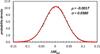 |
Fig. 5. Result of Monte Carlo error propagation: points represent the normalized frequency of Monte Carlo events, while the curve is the best-fit Gauss. function. The mean and standard deviation are shown. |
2.4. Comparisons with previous calculations
In the extant literature there are several papers reporting calculations of RGB stellar models for globular cluster stars. Here, we compare our results with the most recent ones, as obtained with four different evolutionary codes, namely BaSTI (Pietrinferni et al. 2004)5, PGPUC (Valcarce et al. 2012), GARSTEC (Serenelli et al. 2017), and PISA (Dell’Omodarme et al. 2012)6. To perform these comparisons, we computed specific models with the same initial stellar parameters as in the previous calculations. The results of these comparisons are reported in Table 3. In general, the differences in the tip bolometric magnitude are within the quoted 1σ theoretical uncertainty (see Sect. 2.3). However, a larger discrepancy is found with respect to the PGPUC model, the latter being about 0.09 mag fainter (or δ log L/L⊙ = 0.037). Since this model is the same one adopted by Viaux et al. (2013a) to constrain the axion-electron coupling, we attempted to understand the origin of this discrepancy. This faintness of the PGPUC models at the RGB tip was already noted by Serenelli et al. (2017). These authors suggested that it is due to the evaluation of the screening enhancement factors that multiply the nuclear reaction rates. Indeed, Viaux et al. (2013a,b) followed the prescriptions of Salpeter (1954), who developed the theoretical framework for the calculation of the screening potential in the two extreme cases of weak and strong regime of the stellar plasma. In the weak screening regime, the coupling between a nucleus and the nearby electrons and nuclei is weak, or, more precisely, the Coulomb interaction energy is much smaller than the thermal energy (KT). On the other hand, the strong regime refers to the case of strong coupling, that is, Coulomb interaction energy much greater than the thermal energy. The weak regime condition is usually fulfilled in the core of H-burning stars with masses ∼0.8 M⊙. However, at the higher density of the core of an RGB star (∼106 g cm−3), the interaction energy is comparable to the thermal energy, and the weak screening prescription by Salpeter (1954) largely overestimates the screening factors. As shown by Dewitt et al. (1973) and Graboske et al. (1973), the intermediate regime is more appropriate to describe the plasma conditions in the core of an RGB star. As an example, for a He-rich gas of which the temperature and density are 108 MK and 106 g cm−3, respectively, the effective 3α rate is more then a factor of 2 larger when the weak screening is imposed. As a result, the He ignition should occur at lower luminosity. To quantify this effect, we calculated an additional model, M = 0.82 M⊙, Z = 0.00136, and Y = 0.25, by imposing week screening factors for all the nuclear reactions, from the beginning of the evolution up to the RGB tip. As reported in the last column of Table 3, at the RGB tip this model is about 0.075 mag fainter than our reference model computed by calculating the screening factors according to Dewitt et al. (1973) and Graboske et al. (1973). We conclude that most of the discrepancies between our models and the PGPUC ones are likely due to the different nuclear screening prescriptions. As we show in Sect. 4, the larger RGB tip luminosity we obtain by adopting the intermediate screening reduces the need for additional energy loss from the RGB core, and, in turn, it implies a lower upper bound for gae.
Comparisons with previous calculations.
Finally, we wish to mention a discrepancy between our sensitivity study and that discussed in Valle et al. (2013). At variance with our result, these authors find that the major uncertainty affecting the RGB tip luminosity is due to a variation of the radiative opacity. On the other hand, our result confirms previous findings reported by Viaux et al. (2013a) and Serenelli et al. (2017). In principle, the energy transport within the core of an RGB star is mainly driven by the heat conduction from degenerate electrons, so that a 5% variation of the radiative opacity at high temperature is expected to produce a small effect on the tip luminosity. Outside the core, the radiative opacity affects the temperature gradient, which is super-adiabatic in a large portion of the convective envelope. As a result, the effective temperature of an RGB star is modified by a change of the radiative opacity, but its luminosity is only marginally affected. For these reasons, although further investigations are certainly needed to clarify the origin of such a discrepancy, we are quite confident about the robustness of our prediction.
3. Combining HST photometries with those from ground-based telescopes
In this section, we illustrate the strategy we followed to derive the RGB tip bolometric magnitudes from optical (V and I) and near-infrared (J and K) photometries.
3.1. The VI catalog
In order to select the most complete samples of RGB stars, the adopted strategy was to combine different catalogs characterized by complementary properties. In particular, to resolve the crowded central regions, we exploited the high spatial resolution of space-based telescopes, while to sample the entire radial extension of the clusters, we used photometric data from ground-based facilities that cover a larger field of view (FoV). To this aim, the required data sets were extracted from public catalogs, namely the ACS globular cluster survey (Sarajedini et al. 2007) and the homogeneous UBVRI photometry of globular clusters (Stetson et al. 2019). In particular, we used V and I magnitudes from the latter and the magnitudes in the filters F606W and F814W, as calibrated into the ground photometric system, for the former. By using common stars, we carefully checked that the ground system magnitudes tabulated into the HST catalog and those from the ground-based catalogs were homogeneous.
For the present work, we selected three clusters, namely M5, NGC 362 and 47 Tuc. The first is the cluster already used by Viaux et al. (2013b) to constrain the strength of the axion-electron coupling, while the other two clusters are the only ones for which reliable parallax distances are available after the Gaia DR2 (Chen et al. 2018). In the specific case of NGC 362, since the ground-based catalog was not complete as for M5 and 47 Tuc, we have complemented our analysis with additional observations from the ESO archive, that is, FORS2 data from the program 60.A-9203. In particular, we analyzed two short images (1 s each) obtained with the standard resolution (0″.25 pixel−1 for a total FoV of 6′.8 × 6′.8; hereafter SR) and two (1 s each) with a high-resolution (0″.125 pixel−1 for a total FoV of 4′.2 × 4′.2; hereafter HR) collimator in both IBESS and VBESS filters. For both data sets (i.e., HR and SR), the photometric analysis was performed using DAOPHOT II (Stetson 1987). Briefly, for each exposure, we first modeled a spatially variable point spread function using more than 50 isolated and bright stars. We then applied this model to all the sources detected more than 3σ from the background level, and we built the final catalog containing all the sources detected in both filters. Finally, we report the instrumental magnitudes to the absolute reference system by cross-correlation7 with the standard Ste-tson catalog. Then, the combined catalogs were built by joining together the different available catalogs. When possible, we preferentially adopted the HST magnitude, which is not prone to crowding. However, for a few central very bright stars, we nevertheless preferred to adopt the ground based magnitudes, since the HST magnitudes may be biased because of the nonlinear regime close to the photometric saturation level. We note that for such bright objects, the crowding is not a problem, even in the most central regions. In the case of NGC 362, for which two FORS2 data sets were also available, the priority adopted in the catalog compilation was HST, FORS2 HR, FORS2 SR, and Stetson standard, except for very bright objects, for which we adopted the FORS HR magnitudes even if detected in the HST catalog. Finally, we dereddened the magnitudes by adopting the E(B − V) values tabulated in Harris (1996, 2010 version) and a standard extinction law with Rv = 3.1. Following Cardelli et al. (1989) and O’Donnell (1994), we assumed AV = 3.12 E(B − V) and AI = 1.87 E(B − V).
The apparent bolometric magnitudes of the RGB stars were calculated by means of the UBVRIJHK color-temperature calibration reported in Worthey & Lee (2011). In all cases, we assumed log g = 0, which is a typical gravity value for bright RGB stars. Then, we estimated the bolometric correction of all stars making use of their own dereddened color (V − I)0. The combined errors on the bolometric magnitudes were calculated as the propagation of several sources of uncertainty: namely the photometric error as estimated with DAOPHOT, all the sources of errors in the determination of the calibrated and dereddened magnitudes (e.g., the value of reddening E(B − V), the extinction law, the calibration zero points, etc.), and the error on the bolometric correction. The latter includes the intrinsic uncertainty of the BC-color empirical relation by Worthey & Lee (2011) and that of the measured V − I colors. For the brightest RGB stars, this uncertainty is of the order of ±0.15 mag and it represents the major contribution to the mBOL error budget.
3.2. The near-IR catalog
In addition to the VI photometry described in the previous section, we also considered the near-IR catalog of GGCs presented in a series of papers by the Bologna team (Ferraro et al. 2000; Valenti et al. 2004a). The catalog contains a set of JHK photometric data of 22 GGCs, obtained at the ESO MPI 2.2 m telescope equipped with the near-IR camera IRAC-2. These data cover the most central 4 × 4 arcmin2 regions of each cluster. In some cases, additional data from the 2mass survey have been used to sample more external regions (Valenti et al. 2004a). For five clusters, that is, M3, M5, M10, M13, and M92, we also considered the J and K observations obtained by Valenti et al. (2004b) with the Telescopio Nazionale Galileo (TNG) equipped with the ARNICA IR camera. These observations cover the most crowded 1.5 × 1.5 arcmin2 central regions. Finally, a rather large sample of giants belonging to the RGBa of ω Cen, as obtained by Sollima et al. (2004) with the ESO NTT telescope during the commissioning of the SOFI camera, was also used. This data set covers a 13 × 13 arcmin2 area around the cluster center. Then, the bolometric magnitudes were estimated by means of the empirical bolometric corrections derived by Buzzoni et al. (2010). In particular, we used their BCK versus (J–K) color relation. As for the VI photometriic samples, the errors of the bolometric magnitudes were calculated by combining the uncertainties due to the photometry with those affecting the bolometric correction. In general, the K-band bolometric corrections are more reliable than the V and I ones. Following Buzzoni et al. (2010), for the brightest RGB stars, we assumed σBC = ±0.1 mag.
3.3. Selection of RGB stars
Particular attention has been paid to decontaminate the RGB photometric samples from background field stars and from the presence of AGB stars. The selection of RGB star candidates was done based on the available colors and magnitudes (VIJHK). Given the very small photometric errors of RGB and AGB stars (∼0.01 mags) and the expected color separation between the two parent sequences (0.02 < (V − I)RGB − (V − I)AGB < 0.1), we found a clear separation between the two populations from a minimum of 2σ, around 1 mag below the RGB-tip, up to more than 20σ at larger magnitudes. A good example of this RGB-AGB separation can be found in Fig. 1 of Beccari et al. (2006), where the two populations of 47 Tuc, thanks to the high quality of the data similar to that of the present work, are well populated and clearly distinguishable. Such a clear separation allowed us to select the RGB sample through a box selection drawn around the RGB fiducial line and properly checked by a visual inspection.
3.4. The RGB tip luminosity from GGC photometries
In this section, we illustrate the method we followed to determine the luminosity of the RGB tip from a finite photometric sample of RGB stars. This problem is equivalent to the evaluation of the difference of the luminosity of the RGB tip and that of the brightest observed RGB star. To do that, we made use of theoretical luminosity functions (LFs) and synthetic color-magnitude diagrams (SCMDs). First of all, we verified that the observed and the theoretical LFs were drawn from the same distribution. In Fig. 6, the observed luminosity function of the cluster M5 is compared to the theoretical expectation. By means of a classical Kolmogorov-Smirnov test, we found a statistic parameter d = 0.2 and a probability of 97.5% that the theoretical and the observed data sets are drawn from the same distribution. Furthermore, a chi-squared test leads to a 86% probability that the theoretical and the observed LFs are drawn from the same distribution. These statistical tests support our use of the theoretical LFs to evaluate the differences between observed luminosity of the brightest RGB stars and the RGB tip luminosity. Then, synthetic color-magnitude diagrams were generated following a standard Monte Carlo procedure. Some examples are illustrated in Fig. 7. In computing these four SCMDs, we assumed the same input parameters; in particular, the same age, chemical composition, B and V photometric uncertainties, and total number of stars. In all cases, the RGB tip occurs at MV = −2.15 mag. In contrast, the location of the brightest star changes randomly because of statistical fluctuations.
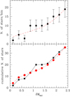 |
Fig. 6. Upper panel: observed luminosity function of the 2.5 mag brightest portion of the RGB of cluster M5 (squares) is compared to the theoretical luminosity function (dashed line). Poisson errors ( |

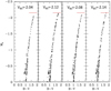 |
Fig. 7. Synthetic color-magnitude diagrams of bright globular cluster stars. All SCMDs were computed with the same input parameters; in particular, the same age, chemical composition, and number of stars. The location of the RGB tip is marked by a red horizontal line. For all the SCMDs, it is at MV = −2.15. The MV mag of the brightest stars are reported in each panel (VBS). |
The analysis of these fluctuations can be done by collecting a sufficient number of these SCMDs, as illustrated in Fig. 8. This frequency histogram represents the distribution of the differences between the bolometric magnitude of the brightest stars and that of the RGB tip in a sample of 105 SCMDs. Each SCMD was computed assuming an age of 13 Gyr, Z = 0.001, and Y = 0.25. In addition, each SCMD contains 100 stars in the brightest 2.5 mag portion of the RGB. The mode of the probability distribution is evidently 0, while the median is ⟨δ⟩100 = 0.030 mag, and the standard deviation from the median is STD = 0.056 mag. However, for probability distributions with a long right tail, the standard deviation overestimates the dispersion. For this reason, the mean deviation from the median (MDM8), or the interquartile range, were often preferred to the STD. For the probability distribution shown in Fig. 8, we find MDM100 = 0.035 mag, while the first and the third quartiles are at −0.019 and +0.033 with respect to the median. We note that the semi-interquartile range is 0.026 mag, which is slightly smaller than MDM and about half the STD. In Table 4, we report the values of medians, standard deviations, and mean deviations from medians, as obtained under different assumptions about age, chemical composition, and the parameter N that represents the number of stars in the brightest portion of the RGB. It results that the statistical descriptors are practically insensitive to variations of age, Y, and Z, within the range expected for globular cluster stars. In contrast, they are substantially affected by the number of bright RGB stars. Then, knowing the bolometric magnitude of the brightest RGB star (mBS) and the number of stars in the brightest 2.5 mag of the observed RGB (N) for each cluster, we can estimate the tip bolometric magnitude as: mtip = mBS − ⟨δ⟩N, where ⟨δ⟩N is the median of the distribution function of mBS − mtip. Concerning the total error, we assumed  , where σBS is the error on the apparent bolometric magnitude of the brightest RGB star (see Sects. 3.1 and 3.2) and MDMN is the mean deviation from the median. We note that in principle mBS − mtip cannot be negative, so the error bar may be asymmetric. However, the assumption of a symmetric error, although it implies a small overestimation of the left side of the uncertainty, has a negligible impact on the final results. For practical purposes, good approximations of median, standard deviation, and mean deviation from the median can be obtained by means of the following equations (valid for 50 ≤ N ≤ 300):


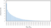 |
Fig. 8. Histogram representing frequency of differences between the bolometric magnitute of the brightest star (MBS) and that of the RGB tip (Mtip) for a sample of 105 SCMDs computed for an age of 13 Gyr, Z = 0.001, Y = 0.25 and with 100 stars within 2.5 mag from the RGB tip. |
Medians, standard deviations, and mean deviations from the median of the corrections applied to the bolometric magnitude of the brightest RGB stars.
where x = log(N). We note that the photometric samples of all 22 of the GGCs we analyzed contain between 50 and 200 stars in the brightest 2.5 mag of the RGB. Clusters with N < 50 have been excluded.
3.5. Cluster parameters: Distance, age, and chemical composition
Comparisons of models with observations require the knowledge of stellar parameters, such as the mass and the initial chemical composition. As is well known, globular cluster stars show substantial deviations from a scaled-solar composition. In particular, α elements, such as O, Mg, Si, and Ca, are enhanced ([α/Fe]> 0). According to Salaris et al. (1993), reliable predictions of the observed stellar properties of α−enhanced globular cluster stars, such as the RGB tip luminosity, can be obtained with models computed assuming a scaled-solar composition with global metallicity9:
![Mathematical equation: $$ \begin{aligned} \left[ \frac{{M}}{{H}} \right] = \left[ \frac{\mathrm{Fe}}{\mathrm{H}} \right]+\log (a\times f_\alpha + b), \end{aligned} $$](/articles/aa/full_html/2020/12/aa38775-20/aa38775-20-eq8.gif) (2)
(2)
where fα = 10[α/Fe] is the α-enhancement factor, while a and b are numerical coefficients that depend on the adopted solar composition. According to the extant spectroscopic analysis of globular cluster stars, the average α-enhancement is [α/Fe] ∼ 0.3, with the most metal-rich clusters showing lower values, and the most metal-poor ones presenting larger enhancements (Carney 1996; Pritzl et al. 2005). In the present work, we adopted the [Fe/H] from Carretta et al. (2009) and assumed [α/Fe] = 0.4, for clusters with [Fe/H]< − 2, [α/Fe] = 0.3, for those with −2 < [Fe/H]< − 0.8, and [α/Fe] = − 0.375[Fe/H], for the more metal-rich ones. Since we adopted the Lodders et al. (2009) solar composition, the numerical coefficients should be: a = 0.6695 and b = 0.3305 (see Piersanti et al. 2007). Owing to the large uncertainty of the metallicity estimation, we assumed a conservative [M/H] error bar of ±0.2. As reported in Table 5, the propagation of this error into the tip bolometric magnitude produces an uncertainty of about ±0.04 mag. The estimated [M/H] value of the 22 clusters in our sample are listed in Col. 2 of Table 6.
Uncertainties of cluster parameters and their effects on the tip bolometric magnitude.
RGB tip bolometric magnitudes as obtained under different assumtion for the distance scale.
Concerning the cluster age, we assumed 13 ± 2 Gyr. Then, for each metallicity, we selected the initial stellar mass corresponding to the assumed age. We note that this uncertainty of the age/mass implies a marginal variation of the estimated tip bolometric magnitude (see Table 5).
For the bulk of the halo stellar population, we assumed a He abundance Y = 0.25 ± 0.01 (Izotov et al. 2014; Aver et al. 2015). On the other hand, the possible presence of He-enhanced stars in the cluster samples should be also considered. According to Milone et al. (2018), the He enhancement of second generation stars in the clusters of our sample is always smaller than δY2G − 1G < 0.03, while the maximum Y variation is generally smaller than δYmax < 0.0510. We note that the RGB tip of He-enhanced stars is fainter than that of stars with normal initial He abundance. In addition, if the age difference between the first and the second generation of stars is negligible, the second generation RGB stars, due to the higher initial He content, should have smaller masses. This occurrence partially counterbalances the decrease of the tip luminosity caused by the He enhancement in second generation stars. To quantify this effect, we calculated a few He-enhanced models by reducing the initial mass in order to keep their age equal to that of normal He stars (13 Gyr). In practice, assuming a maximum He variation among the stars of the same cluster of δY = 0.05, the result is that the RGB tip of the most He-enhanced stars would be 0.037 mag fainter than that with normal He. Therefore, if the stars of the first generation are not a minority, the brightest RGB stars are those with normal He. However, in the case of an overwhelming majority of He-enhanced stars, higher statistical fluctuations of the observed tip luminosity are possible. In order to take into account such a possibility, in the analysis discussed in the next section we include an additional error affecting the tip magnitude due to the Y variations illustrated here. As reported in Table 5, our conservative estimation of this error is σY = 0.045, which corresponds to the systematic shift of the tip luminosity when the He content changes from Y = 0.24 to Y = 0.30 (or δY = 0.06).
Comparisons of theoretical and observed luminosities also require the knowledge of the cluster distances. Among the classical methods used to derive the distance to clusters, those based on the location in the color-magnitude diagram of the horizontal branch are widely exploited (Harris 1996, 2010; Ferraro et al. 1999). In particular, the mean luminosity of the horizontal branch or that of the zero-age horizontal branch (ZAHB) are often adopted as calibrated candles. Since the horizontal branch luminosity depends on the chemical composition, either empirical or theoretical MV(ZAHB)−metallicity relations are used. Several alternative methods have also been investigated, such as those based on main- or white-dwarf-sequence fitting, pulsation properties of RR Lyrae stars, or orbital parameters of eclipsing binaries, even if their application is often limited to smaller sub-samples of the GGCs (for a complete review of these methods, see Harris 2010). Recently, the possibility of obtaining very precise parallax measurements with the Gaia astrometric satellite has been widely anticipated (Pancino et al. 2017). After the second data release (Gaia DR2), however, it has been realized that for faint sources (G > 14 mag), the Gaia parallaxes are affected by significant systematic errors. In particular, these systematics substantially affect the derivation of distance to GGCs. Nevertheless, Chen et al. (2018, CH2018) were able to obtain quite accurate distances of two GGCs, NGC 362 and 47 Tuc, taking advantage of the background stars in the Small Magellanic Cloud and quasars to account for parallax systematics. Moreover, an indirect distance estimation of a large sample of GGCs was recently obtained by Baumgardt et al. (2019, B2019). Combining proper motion and radial velocity measurements from the Gaia DR2 with ground-based measurements of line-of-sight velocities, they obtained distances by fitting N-body GGC models to the observed kinematic properties.
In our analysis, we make use of the distance moduli we obtained following the method described in Ferraro et al. (1999) to determine the observed ZAHB luminosity. However, at variance with Ferraro et al. (1999), we used a semi-empirical MV(ZAHB)−metallicity relation. In practice, we adopted the relation reported in Eq. (4) of Ferraro et al. (1999) to describe the quadratic dependence of MV(ZAHB) from the metallicity, but the zero point was re-calibrated in such a way so as to reproduce the absolute MV(ZAHB) of NGC 362 and 47 Tuc, for which precise distances from Gaia parallaxes are available. A weighted average of the two zero points was adopted: namely, 1.03 ± 0.07 mag.
The distance moduli of the 22 clusters in our sample are reported in Table 6. In particular, Column 3 features the distance moduli based on the observed ZAHB luminosity, while in Cols. 4 and 5, one can see those based on Gaia parallax and kinematic measurements, as obtained by Chen et al. (2018) and Baumgardt et al. (2019), respectively. We note that for the ZAHB distances, we assumed a conservative common error of ±0.2 mag, even if it may be smaller for some clusters. It includes the uncertainties in the determination of the ZAHB V magnitudes and the one due to the adopted zero point of the MV(ZAHB)−metallicity relation.
4. Results
The RGB tip bolometric magnitude of 22 GGCs, as estimated under different assumptions for the distances and the photometric samples, are listed in Cols. 6–8 of Table 6. Here, the 1σ error includes the uncertainty due to; (i) the observed apparent magnitude (Sects. 3.1 and 3.2), (ii) the statistical fluctuations of the magnitudes of the brightest RGB stars (Sect. 3.4), and (iii) the cluster distance (Sect. 3.5). Figure 9 compares the tip bolometric magnitudes obtained by assuming the distance moduli based on the observed ZAHB with those derived by means of the kinematic properties. With a few exceptions, the differences are generally smaller than the quoted errors. For 47 Tuc, which is one of the two clusters for which we have the most complete sample of bright stars, that is, VIJHK data of about 200 stars in the brightest 2.5 magnitude of the RGB, the kinematic distance modulus practically coincides with that obtained from the Gaia parallax (and from the ZAHB luminosity), while for NGC 362 it is 0.16 mag larger. For the third best studied cluster, M5, we do not have a reliable estimation of the parallax, but the distance estimated from the ZAHB is in excellent agreement with that obtained by fitting the kinematic properties. Observed and predicted tip bolometric magnitudes are compared in Fig. 10. The black solid line represents our theoretical prediction for g13 = 0 (no axions), while the dotted line is the linear regression of the 22 data points (squares). The latter is about 0.04 mag brighter than the theoretical expectation (at [M/H] = − 1). This difference could be interpreted as a hint in favor of a small extra cooling, even if it is of the same order of magnitude of the estimated theoretical error. In any case, the axion-electron coupling should be very weak. The theoretical expectation for g13 = 4 is also shown (black dashed line). We note that this value of the axion-electron coupling is indicative of the previous upper bound obtained by Viaux et al. (2013a). The observed tip bolometric magnitudes clearly exclude such a large coupling.
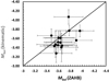 |
Fig. 9. Tip bolometric magnitudes of 16 GGCs obtained by assuming the ZAHB distance scale (horizontal axis) are compared to those obtained assuming the kinematic distances (verical axis), as derived by Baumgardt et al. (2019). |
 |
Fig. 10. Tip bolometric magnitude derived from optical and IR photometry of 22 GGCs (red circles) are compared to our theoretical predictions for g13 = 0 (black solid line) and g13 = 4 (black dashed line). The red dotted line represents the least-squares fit of the 22 observed Mbol. |
In order to estimate the most probable value of g13 and its upper bound, we have calculated, for each cluster in our sample, the following probability functions:

where
![Mathematical equation: $$ \begin{aligned} f_j = \exp \left[- \frac{(M_{\rm obs}-M_{\rm theo}(g_{13}))^2}{\sigma ^2_{\rm obs}+\sigma ^2_{\rm theo}+\sigma ^2_{\rm age}+\sigma ^2_{Y}+\sigma ^2_{[M/H]}} \right], \end{aligned} $$](/articles/aa/full_html/2020/12/aa38775-20/aa38775-20-eq10.gif)
and
is a normalization factor. Here, σobs are the errors of the tip absolute magnitude reported in Table 6, while σtheo represents the cumulative theoretical uncertainty (see Sect. 2.1). In addition, we also considered the uncertainties on the chemical composition, that is, Y and [M/H], and that on the cluster age (see Sect. 3.5 and Table 5). Then, the cumulative likelihood is:
where Δ is a vector containing the difference between the observed and the predicted tip bolometric magnitude, and C is the error matrix. The latter has been computed following the procedure described in D’Agostini (1994). In particular, we considered the covariance due to the correlations introduced by the calibration of the zero point of the distance scale and bolometric corrections, as well as that due to the theoretical uncertainties (see Sects. 2.3 and 3.5).
The lj probability functions for the three best studied clusters (M5, 47 Tuc, and NGC362) are shown in Fig. 11. We note that for these three clusters, both optical and near-IR photometric samples are available. Furthermore, the observed tip bolometric magnitude adopted here is a weighted average of those independently obtained from the VI and the JK samples. Similarly, the cumulative likelihood functions, as obtained by assuming the ZAHB distances (22 clusters, solid line) or the kinematic distances (16 clusters, dashed line) are shown in Fig. 12.
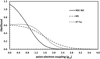 |
Fig. 11. Likelihood functions for M5, 47 Tuc, and NGC 362. |
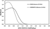 |
Fig. 12. Cumulative likelihood functions, as obtained under different assumptions for the distance scale. |
The best values and the upper bounds for the axion-electron coupling (g13) are reported in Cols. 4 and 5 of Table 7. The upper bounds were obtained by imposing the conditions:
Results of likelihood analysis.
where u.b. is the g13 upper bound. In practice, values of g13 greater than u.b. are excluded with 95% confidence.
The two distance scales lead to a similar conclusion: namely, there is a hint of a weak axion-electron coupling, g13 ∼ 0.05, with a stringent upper bound of g13 < 1.5 (95% confidence).
5. Conclusions
Based on VIJK photometries of bright RGB stars and state-of-the-art distance and metallicity scales, we determined the absolute magnitude of the RGB tip for a sample of 22 GGCs. An accurate evaluation of all the uncertainties was performed. We also revised the corresponding model predictions by analyzing the present theoretical and experimental knowledge of the relevant input physics, such as nuclear reactions, neutrino emission rates, thermodynamic properties of stellar plasma and the like. These theoretical predictions are, in general, in good agreement with the observed tip bolometric magnitudes, even if the latter are ∼0.04 mag brighter, on average. This small shift between theoretical and observed tip bolometric magnitude could be the consequence of a weak axion-electron coupling. Following this hypothesis, we computed additional stellar models by including the production of thermal axions. We note that due to the high electron degeneracy, Bremsstrahlung is the most relevant thermal process capable of producing a sizeable flux of axions from the core of RGB stars. Therefore, by means of a cumulative likelihood analysis, as obtained considering all 22 clusters of our sample, we estimated the coupling parameter that determines the strength of the energy sink induced by the production of Bremsstrahlung axion. We find that the likelihood probability is maximized for  . Moreover, we find an upper bound for this parameter of gae = 1.48 × 10⁻¹³, with 95% confidence.
This new bound represents the more stringent constraint for the axion-electron coupling available so far. Indeed, in addition to the work of Viaux et al. (2013a), who reported gae < 4.3 × 10⁻¹³ from the luminosity of the RGB tip of the globular cluster M5, other astrophysical constraints we find in the extant literature are those of Miller Bertolami et al. (2014, see also Isern 2018), reporting gae < 2.8 × 10⁻¹³, as obtained from an analysis of the white dwarf (WD) luminosity functions, and Córsico et al. (2016), who found gae < 7 × 10⁻¹³, from the period drift of pulsating WDs.
Concerning the direct search for axions, recent years have seen impressive experimental efforts (for a review of the axion experimental landscape, see Irastorza & Redondo 2018; DiLuzio et al. 2020b, and Sikivie 2020). However, the axion coupling to electrons is particularly difficult to probe experimentally. The most stringent upper bounds have been obtained by the XENON100 collaboration (Aprile et al. 2014), gae < 7.7 × 10⁻¹² (90% CL), LUX (Akerib 2017), gae < 3.5 × 10⁻¹², and PandaX-II (Fu et al. 2017), gae < 4 × 10⁻¹². These bounds are not yet competitive with the stellar bounds on this coupling.
Before submitting the present paper, there was an announcement from the XENON1T collaboration of a possible detection of solar axions (Aprile et al. 2020). For values of the axion-photon coupling not excluded by previous experiments (e.g., Anastassopoulos et al. 2017), they find 27 < gae/1013 < 37 (90% confidence), a value at least 20 times higher than the upper bound we obtained in this work (see also Di Luzio et al. 2020a). Alternative interpretations of the signal detected by XENON1T have already been proposed (see the discussion in Aprile et al. 2020), among which the possibility that this signal is due to a dark matter ALP with mass of a few keV and a coupling-to-electron gae ∼ 10−13 (Takahashi et al. 2020). In that case, these ALPs may constitute all or a fraction of the local dark matter. Such an explanation would remove the tension of the XENON1T detection with our work.
Finally, we remark that the present upper bound for the axion-electron coupling remains valid also in the case of additional energy sinks active during the RGB evolutionary phase, not included in the present models, such as a nonzero neutrino magnetic moment or a sizeable axion coupling with photons. On the contrary, the existence of these additional energy sinks would affect the hint on gae. For example, in Sect. 2.2, we recall that at the high density of the core of an RGB star, the Primakoff process is suppressed. Nevertheless, its effect on the RGB tip luminosity may be not completely negligible. In the most extreme case of an axion-photon coupling of gaγ = 6 × 10⁻¹¹ GeV−1, that is, the upper bound independently obtained from the solar axions by the CAST collaboration (Anastassopoulos et al. 2017) and from the horizontal branch lifetimes (Ayala et al. 2014), the resulting upward shift of the RGB tip would explain most of the small difference between the standard theoretical predictions (no axions) and the least-squares fit of the observed tip luminosity (the solid and the dotted curves in Fig. 10). In this framework, we cannot exclude a much smaller (at least 0) axion-electron coupling.
In a recent paper (Straniero et al. 2019), we reviewed the axion production processes in stellar interiors and we provided the corresponding energy-loss rate to be used in stellar model calculations.
See, in particular, Sect. 2 and the Appendix.
The same algorithms are also valid for the production of more general ALPs. Therefore, the conclusions of the present work apply to axions as well as to ALPs.
The possible existence of a nonzero neutrino magnetic moment, which would imply systematic increases of the energy-loss rates, is not considered here (see Sect. 5).
To perform the cross-correlation, we used CataXcorr, a code aimed at cross-correlating catalogs and finding astrometric solutions, developed by P. Montegriffo at INAF – OAS Bologna. This package has been successfully used in a large number of papers in the past years, in particular, Pallanca et al. (2013, 2014, 2019), Cadelano et al. (2017), and Dalessandro et al. (2014).
 , where δi is the brightest star-to-tip difference for the i SCMD, n is the total number of SCMDs, and N is the number of stars in the brightest 2.5 mag of the RGB.
As usual, the global metallicity ([M/H]) and the total mass fraction of the elements with atomic number ≥6 (Z) are related by [M/H] = log(Z/X)−log(Z/X)⊙.
A larger maximum variation (0.081) is quoted for NGC 6461, but it is affected by a large uncertainty (±0.22).
Acknowledgments
We are in debt with F. Capozzi and G. Raffelt for a careful reading of our manuscript. We acknowledge that after our submission to A&A, they uploaded on the ArXiv an independent study where they reached conclusions similar to ours. Our work has been supported by the Agenzia Spaziale Italiana (ASI) and the Instituto Nazionale di Astrofsica (INAF) under the agree-ment n. 2017-14-H.0 - attività di studio per la comunità scientifica di Astrofisica delle Alte Energie e Fisica Astroparticellare. I.D. research is also supported by the MICINN-FEDER project PGC2018-095317-B-C21, while A. M. is partially supported by the Istituto Nazionale di Fisica Nucleare (INFN), through the “Theoretical Astroparticle Physics” project, and by the research grant number 2017W4HA7S: “Neutrino and Astroparticle Theory Network”, under the program PRIN 2017 funded by the Italian Ministero dell’Universitá e della Ricerca (MUR).
References
- Adelberger, E. G., García, A., Robertson, R. G. H., et al. 2011, Rev. Mod. Phys., 83, 195 [NASA ADS] [CrossRef] [Google Scholar]
- Akerib, D. S., Alsum, S., Aquino, C., et al. 2017, Phys. Rev. Lett., 118, 261301 [CrossRef] [Google Scholar]
- Anastassopoulos, V., Aune, S., Barth, K., et al. 2017, Nat. Phys., 13, 584 [CrossRef] [Google Scholar]
- Angulo, C., Arnould, M., Rayet, M., et al. 1999, Nucl. Phys. A, 656, 3 [NASA ADS] [CrossRef] [Google Scholar]
- Aprile, E., Agostini, F., Alfonsi, M., et al. 2014, Phys. Rev. D, 90, 062009 [CrossRef] [Google Scholar]
- Aprile, E., Aalbers, J., Agostini, F., et al. 2020, Phys. Rev. D, 102, 072004 [CrossRef] [Google Scholar]
- Aver, E., Olive, K. A., & Skillman, E. D. 2015, J. Cosmol. Astropart. Phys., 2015, 011 [NASA ADS] [CrossRef] [Google Scholar]
- Ayala, A., Domínguez, I., Giannotti, M., Mirizzi, A., & Straniero, O. 2014, Phys. Rev. Lett., 113, 191302 [NASA ADS] [CrossRef] [Google Scholar]
- Baumgardt, H., Hilker, M., Sollima, A., & Bellini, A. 2019, MNRAS, 482, 5138 [Google Scholar]
- Beaudet, G., Petrosian, V., & Salpeter, E. E. 1967, ApJ, 150, 979 [NASA ADS] [CrossRef] [Google Scholar]
- Beccari, G., Ferraro, F. R., Lanzoni, B., & Bellazzini, M. 2006, ApJ, 652, L121 [NASA ADS] [CrossRef] [Google Scholar]
- Buzzoni, A., Patelli, L., Bellazzini, M., Pecci, F. F., & Oliva, E. 2010, MNRAS, 403, 1592 [NASA ADS] [CrossRef] [Google Scholar]
- Cadelano, M., Dalessandro, E., Ferraro, F. R., et al. 2017, ApJ, 836, 170 [NASA ADS] [CrossRef] [Google Scholar]
- Cardelli, J. A., Clayton, G. C., & Mathis, J. S. 1989, ApJ, 345, 245 [NASA ADS] [CrossRef] [Google Scholar]
- Carney, B. W. 1996, PASP, 108, 900 [NASA ADS] [CrossRef] [Google Scholar]
- Carretta, E., Bragaglia, A., Gratton, R., D’Orazi, V., & Lucatello, S. 2009, A&A, 508, 695 [NASA ADS] [CrossRef] [EDP Sciences] [Google Scholar]
- Chaboyer, B., Deliyannis, C. P., Demarque, P., et al. 1992, ApJ, 388, 372 [NASA ADS] [CrossRef] [Google Scholar]
- Chen, S., Richer, H., Caiazzo, I., & Heyl, J. 2018, ApJ, 867, 132 [NASA ADS] [CrossRef] [Google Scholar]
- Córsico, A. H., Romero, A. D., Althaus, L. G., et al. 2016, JCAP, 7, 036 [NASA ADS] [CrossRef] [Google Scholar]
- Cox, J., & Giuli, R. 1968, Principles of Stellar Structure: Applications to Stars, Principles of Stellar Structure (Gordon and Breach) [Google Scholar]
- Cyburt, R. H., Amthor, A. M., Ferguson, R., et al. 2010, ApJS, 189, 240 [NASA ADS] [CrossRef] [Google Scholar]
- D’Agostini, G. 1994, Nucl. Instrum. Methods Phys. Res. A, 346, 306 [NASA ADS] [CrossRef] [Google Scholar]
- Dalessandro, E., Pallanca, C., Ferraro, F. R., et al. 2014, ApJ, 784, L29 [CrossRef] [Google Scholar]
- Delahaye, F., & Pinsonneault, M. 2005, ApJ, 625, 563 [CrossRef] [Google Scholar]
- Dell’Omodarme, M., Valle, G., Degl’Innocenti, S., & Prada Moroni, P. G. 2012, A&A, 540, A26 [NASA ADS] [CrossRef] [EDP Sciences] [Google Scholar]
- Dewitt, H. E., Graboske, H. C., & Cooper, M. S. 1973, ApJ, 181, 439 [NASA ADS] [CrossRef] [Google Scholar]
- Dicus, D. A., Kolb, E. W., Schramm, D. N., & Tubbs, D. L. 1976, ApJ, 210, 481 [NASA ADS] [CrossRef] [Google Scholar]
- Di Luzio, L., Fedele, M., Giannotti, M., Mescia, F., & Nardi, E. 2020a, Phys. Rev. Lett., 125, 131804 [CrossRef] [Google Scholar]
- Di Luzio, L., Giannotti, M., Nardi, E., & Visinelli, L. 2020b, Phys. Rep., 870, 1 [CrossRef] [Google Scholar]
- Ferraro, F. R., Messineo, M., Fusi Pecci, F., et al. 1999, AJ, 118, 1738 [NASA ADS] [CrossRef] [Google Scholar]
- Ferraro, F. R., Montegriffo, P., Origlia, L., & Fusi Pecci, F. 2000, AJ, 119, 1282 [NASA ADS] [CrossRef] [Google Scholar]
- Formicola, A., Imbriani, G., Costantini, H., et al. 2004, Phys. Lett. B, 591, 61 [NASA ADS] [CrossRef] [Google Scholar]
- Freedman, W. L., Madore, B. F., Hoyt, T., et al. 2020, ApJ, 891, 57 [Google Scholar]
- Fu, C., Zhou, X., Chen, X., et al. 2017, Phys. Rev. Lett., 119, 181806 [CrossRef] [Google Scholar]
- Fynbo, H. O. U., Diget, C. A., Bergmann, U. C., et al. 2005, Nature, 433, 136 [NASA ADS] [CrossRef] [PubMed] [Google Scholar]
- Goriely, S., Hilaire, S., & Koning, A. J. 2008, A&A, 487, 767 [NASA ADS] [CrossRef] [EDP Sciences] [Google Scholar]
- Graboske, H. C., Dewitt, H. E., Grossman, A. S., & Cooper, M. S. 1973, ApJ, 181, 457 [NASA ADS] [CrossRef] [Google Scholar]
- Haft, M., Raffelt, G., & Weiss, A. 1994, ApJ, 425, 222 [NASA ADS] [CrossRef] [Google Scholar]
- Harris, W. E. 1996, AJ, 112, 1487 [NASA ADS] [CrossRef] [Google Scholar]
- Harris, W. E. 2010, ArXiv e-prints [arXiv:1012.3224] [Google Scholar]
- Iglesias, C. A., & Rogers, F. J. 1996, ApJ, 464, 943 [NASA ADS] [CrossRef] [Google Scholar]
- Imbriani, G., Costantini, H., Formicola, A., et al. 2004, A&A, 420, 625 [NASA ADS] [CrossRef] [EDP Sciences] [Google Scholar]
- Irastorza, I. G., & Redondo, J. 2018, Progress in Particle and Nuclear Physics, 102, 89 [CrossRef] [Google Scholar]
- Itoh, N., Totsuji, H., Ichimaru, S., & Dewitt, H. E. 1979, ApJ, 234, 1079 [NASA ADS] [CrossRef] [Google Scholar]
- Itoh, N., Hayashi, H., Nishikawa, A., & Kohyama, Y. 1996, ApJS, 102, 411 [NASA ADS] [CrossRef] [Google Scholar]
- Izotov, Y. I., Thuan, T. X., & Guseva, N. G. 2014, MNRAS, 445, 778 [NASA ADS] [CrossRef] [Google Scholar]
- Kiss, L. L., & Bedding, T. R. 2003, MNRAS, 343, L79 [NASA ADS] [CrossRef] [Google Scholar]
- Krishna Swamy, K. S. 1966, ApJ, 145, 174 [NASA ADS] [CrossRef] [Google Scholar]
- Lederer, M. T., & Aringer, B. 2009, A&A, 494, 403 [NASA ADS] [CrossRef] [EDP Sciences] [Google Scholar]
- Lemut, A., Bemmerer, D., Confortola, F., et al. 2006, Phys. Lett. B, 634, 483 [NASA ADS] [CrossRef] [Google Scholar]
- Lodders, K., Palme, H., & Gail, H. P. 2009, Landolt Börnstein, 712 [Google Scholar]
- Miller Bertolami, M. M., Melendez, B. E., Althaus, L. G., & Isern, J. 2014, JCAP, 10, 069 [NASA ADS] [CrossRef] [Google Scholar]
- Milone, A. P., Marino, A. F., Renzini, A., et al. 2018, MNRAS, 481, 5098 [NASA ADS] [CrossRef] [Google Scholar]
- O’Donnell, J. E. 1994, ApJ, 422, 158 [NASA ADS] [CrossRef] [Google Scholar]
- Pallanca, C., Lanzoni, B., Dalessandro, E., et al. 2013, ApJ, 773, 127 [CrossRef] [Google Scholar]
- Pallanca, C., Ransom, S. M., Ferraro, F. R., et al. 2014, ApJ, 795, 29 [CrossRef] [Google Scholar]
- Pallanca, C., Ferraro, F. R., Lanzoni, B., et al. 2019, ApJ, 882, 159 [CrossRef] [Google Scholar]
- Pancino, E., Bellazzini, M., Giuffrida, G., & Marinoni, S. 2017, MNRAS, 467, 412 [NASA ADS] [Google Scholar]
- Peccei, R. D., & Quinn, H. R. 1977, Phys. Rev. Lett., 38, 1440 [NASA ADS] [CrossRef] [Google Scholar]
- Piersanti, L., Straniero, O., & Cristallo, S. 2007, A&A, 462, 1051 [NASA ADS] [CrossRef] [EDP Sciences] [Google Scholar]
- Piersanti, L., Cristallo, S., & Straniero, O. 2013, ApJ, 774, 98 [NASA ADS] [CrossRef] [Google Scholar]
- Pietrinferni, A., Cassisi, S., Salaris, M., & Castelli, F. 2004, ApJ, 612, 168 [NASA ADS] [CrossRef] [Google Scholar]
- Potekhin, A. Y. 1999, A&A, 351, 787 [NASA ADS] [Google Scholar]
- Potekhin, A. Y., Baiko, D. A., Haensel, P., & Yakovlev, D. G. 1999, A&A, 346, 345 [NASA ADS] [Google Scholar]
- Prada Moroni, P. G., & Straniero, O. 2002, ApJ, 581, 585 [NASA ADS] [CrossRef] [Google Scholar]
- Pritzl, B. J., Venn, K. A., & Irwin, M. 2005, AJ, 130, 2140 [NASA ADS] [CrossRef] [Google Scholar]
- Proffitt, C. R., & Vandenberg, D. A. 1991, ApJS, 77, 473 [NASA ADS] [CrossRef] [Google Scholar]
- Raffelt, G. G. 1996, Stars as Laboratories for Fundamental Physics: The Astrophysics of Neutrinos, Axions, and Other Weakly Interacting Particles (University of Chicago Press) QB464.2.R34 1996 [Google Scholar]
- Raffelt, G., & Weiss, A. 1995, Phys. Rev. D, 51, 1495 [NASA ADS] [CrossRef] [Google Scholar]
- Rogers, F. J., Swenson, F. J., & Iglesias, C. A. 1996, ApJ, 456, 902 [NASA ADS] [CrossRef] [Google Scholar]
- Salaris, M., Chieffi, A., & Straniero, O. 1993, ApJ, 414, 580 [NASA ADS] [CrossRef] [Google Scholar]
- Sallaska, A. L., Iliadis, C., Champange, A. E., et al. 2013, ApJS, 207, 18 [NASA ADS] [CrossRef] [Google Scholar]
- Salpeter, E. E. 1954, Aust. J. Phys., 7, 373 [NASA ADS] [CrossRef] [Google Scholar]
- Sarajedini, A., Bedin, L. R., Chaboyer, B., et al. 2007, AJ, 133, 1658 [NASA ADS] [CrossRef] [Google Scholar]
- Serenelli, A., Weiss, A., Cassisi, S., Salaris, M., & Pietrinferni, A. 2017, A&A, 606, A33 [NASA ADS] [CrossRef] [EDP Sciences] [Google Scholar]
- Sikivie, P. 2020, Rev. Mod. Phys., submitted [arXiv:2003.02206] [Google Scholar]
- Sollima, A., Ferraro, F. R., Origlia, L., Pancino, E., & Bellazzini, M. 2004, A&A, 420, 173 [NASA ADS] [CrossRef] [EDP Sciences] [Google Scholar]
- Stetson, P. B. 1987, PASP, 99, 191 [Google Scholar]
- Stetson, P. B., Pancino, E., Zocchi, A., Sanna, N., & Monelli, M. 2019, MNRAS, 485, 3042 [NASA ADS] [CrossRef] [Google Scholar]
- Straniero, O. 1988, A&AS, 76, 157 [NASA ADS] [Google Scholar]
- Straniero, O., Chieffi, A., & Limongi, M. 1997, ApJ, 490, 425 [NASA ADS] [CrossRef] [Google Scholar]
- Straniero, O., Gallino, R., & Cristallo, S. 2006, Nucl. Phys. A, 777, 311 [NASA ADS] [CrossRef] [Google Scholar]
- Straniero, O., Dominguez, I., Piersanti, L., Giannotti, M., & Mirizzi, A. 2019, ApJ, 881, 158 [CrossRef] [Google Scholar]
- Takahashi, F., Yamada, M., & Yin, W. 2020, Phys. Rev. Lett., 125, 161801 [CrossRef] [Google Scholar]
- Thoul, A. A., Bahcall, J. N., & Loeb, A. 1994, ApJ, 421, 828 [NASA ADS] [CrossRef] [Google Scholar]
- Turcotte, S., Richer, J., Michaud, G., et al. 1998, ApJ, 504, 539 [NASA ADS] [CrossRef] [Google Scholar]
- Valcarce, A. A. R., Catelan, M., & Sweigart, A. V. 2012, A&A, 547, A5 [NASA ADS] [CrossRef] [EDP Sciences] [Google Scholar]
- Valenti, E., Ferraro, F. R., & Origlia, L. 2004a, MNRAS, 351, 1204 [NASA ADS] [CrossRef] [Google Scholar]
- Valenti, E., Ferraro, F. R., Perina, S., & Origlia, L. 2004b, A&A, 419, 139 [NASA ADS] [CrossRef] [EDP Sciences] [Google Scholar]
- Valle, G., Dell’Omodarme, M., Prada Moroni, P. G., & Degl’Innocenti, S. 2013, A&A, 549, A50 [NASA ADS] [CrossRef] [EDP Sciences] [Google Scholar]
- Viaux, N., Catelan, M., Stetson, P. B., et al. 2013a, Phys. Rev. Lett., 111, 231301 [NASA ADS] [CrossRef] [PubMed] [Google Scholar]
- Viaux, N., Catelan, M., Stetson, P. B., et al. 2013b, A&A, 558, A12 [NASA ADS] [CrossRef] [EDP Sciences] [Google Scholar]
- Weinberg, S. 1978, Phys. Rev. Lett., 40, 223 [Google Scholar]
- Wilczek, F. 1978, Phys. Rev. Lett., 40, 279 [NASA ADS] [CrossRef] [Google Scholar]
- Worthey, G., & Lee, H.-C. 2011, ApJS, 193, 1 [NASA ADS] [CrossRef] [EDP Sciences] [Google Scholar]
- Xu, Y., Takahashi, K., Goriely, S., et al. 2013, Nucl. Phys., A, 918 [Google Scholar]
All Tables
Theoretical predictions of the tip bolometric magnitudes for globular cluster models with age = 13 Gyr and Y = 0.25.
Uncertainties of the input physics adopted in the calculations of the tip bolometric magnitudes.
Medians, standard deviations, and mean deviations from the median of the corrections applied to the bolometric magnitude of the brightest RGB stars.
Uncertainties of cluster parameters and their effects on the tip bolometric magnitude.
RGB tip bolometric magnitudes as obtained under different assumtion for the distance scale.
All Figures
|
Fig. 1. 14N(p, γ)15O reaction rates suggested by the collaborations NACRE II and Solar Fusion are compared to the rate reported in the STARLIB repository. |
| In the text | |
|
Fig. 2. Upper panel: evolution of ratio between axion and neutrino luminosites, from the base of the RGB (log L/L⊙ = 1) to the RGB tip, for a model with M = 0.82 M⊙, Y = 0.25, and Z = 0.001. Only the coupling with electrons has been switched on (g13 = 1). Lower panel: evolution of the ratio between Bremsstrahlung and Compton axion luminosities. |
| In the text | |
|
Fig. 3. Neutrinos and axions energy-loss rate within the core of a RGB model close to the RGB tip (just before the He ignition). Model parameters as in Fig. 2. |
| In the text | |
|
Fig. 4. Relation Mbol at the RGB tip versus g13 for 3 different metallicities ([M/H]). |
| In the text | |
|
Fig. 5. Result of Monte Carlo error propagation: points represent the normalized frequency of Monte Carlo events, while the curve is the best-fit Gauss. function. The mean and standard deviation are shown. |
| In the text | |
|
Fig. 6. Upper panel: observed luminosity function of the 2.5 mag brightest portion of the RGB of cluster M5 (squares) is compared to the theoretical luminosity function (dashed line). Poisson errors ( |
| In the text | |
|
Fig. 7. Synthetic color-magnitude diagrams of bright globular cluster stars. All SCMDs were computed with the same input parameters; in particular, the same age, chemical composition, and number of stars. The location of the RGB tip is marked by a red horizontal line. For all the SCMDs, it is at MV = −2.15. The MV mag of the brightest stars are reported in each panel (VBS). |
| In the text | |
|
Fig. 8. Histogram representing frequency of differences between the bolometric magnitute of the brightest star (MBS) and that of the RGB tip (Mtip) for a sample of 105 SCMDs computed for an age of 13 Gyr, Z = 0.001, Y = 0.25 and with 100 stars within 2.5 mag from the RGB tip. |
| In the text | |
|
Fig. 9. Tip bolometric magnitudes of 16 GGCs obtained by assuming the ZAHB distance scale (horizontal axis) are compared to those obtained assuming the kinematic distances (verical axis), as derived by Baumgardt et al. (2019). |
| In the text | |
|
Fig. 10. Tip bolometric magnitude derived from optical and IR photometry of 22 GGCs (red circles) are compared to our theoretical predictions for g13 = 0 (black solid line) and g13 = 4 (black dashed line). The red dotted line represents the least-squares fit of the 22 observed Mbol. |
| In the text | |
|
Fig. 11. Likelihood functions for M5, 47 Tuc, and NGC 362. |
| In the text | |
|
Fig. 12. Cumulative likelihood functions, as obtained under different assumptions for the distance scale. |
| In the text | |
Current usage metrics show cumulative count of Article Views (full-text article views including HTML views, PDF and ePub downloads, according to the available data) and Abstracts Views on Vision4Press platform.
Data correspond to usage on the plateform after 2015. The current usage metrics is available 48-96 hours after online publication and is updated daily on week days.
Initial download of the metrics may take a while.