| Issue |
A&A
Volume 644, December 2020
|
|
|---|---|---|
| Article Number | A165 | |
| Number of page(s) | 15 | |
| Section | Planets and planetary systems | |
| DOI | https://doi.org/10.1051/0004-6361/202038204 | |
| Published online | 16 December 2020 | |
Solid tidal friction in multi-layer planets: Application to Earth, Venus, a Super Earth and the TRAPPIST-1 planets
Potential approximation of a multi-layer planet as a homogeneous body
1
Observatoire de Genève, Université de Genève,
51 Chemin des Maillettes,
1290
Sauverny, Switzerland
e-mail: This email address is being protected from spambots. You need JavaScript enabled to view it.
2
AIM, CEA, CNRS, Université Paris-Saclay, Université Paris Diderot, Sorbonne Paris Cité,
91191
Gif- sur-Yvette, France
3
Laboratoire de Planétologie et Géodynamique, UMR-CNRS 6112, Université de Nantes,
44322
Nantes cedex 03, France
Received:
20
April
2020
Accepted:
7
October
2020
Abstract
With the discovery of TRAPPIST-1 and its seven planets residing within 0.06 au, it is becoming increasingly necessary to carry out correct treatments of tidal interactions. The eccentricity, rotation, and obliquity of the planets of TRAPPIST-1 do indeed result from the tidal evolution over the lifetime of the system. Tidal interactions can also lead to tidal heating in the interior of the planets (as for Io), which may then be responsible for volcanism or surface deformation. In the majority of studies aimed at estimating the rotation of close-in planets or their tidal heating, the planets are considered as homogeneous bodies and their rheology is often taken to be a Maxwell rheology. Here, we investigate the impact of taking into account a multi-layer structure and an Andrade rheology in the way planets dissipate tidal energy as a function of the excitation frequency. We use an internal structure model, which provides the radial profile of structural and rheological quantities (such as density, shear modulus, and viscosity) to compute the tidal response of multi-layered bodies. We then compare the outcome to the dissipation of a homogeneous planet (which only take a uniform value for shear modulus and viscosity). We find that for purely rocky bodies, it is possible to approximate the response of a multi-layer planet by that of a homogeneous planet. However, using average profiles of shear modulus and viscosity to compute the homogeneous planet response leads to an overestimation of the averaged dissipation. We provide fitted values of shear modulus and viscosity that are capable of reproducing the response of various types of rocky planets. However, we find that if the planet has an icy layer, its tidal response can no longer be approximated by a homogeneous body because of the very different properties of the icy layers (in particular, their viscosity), which leads to a second dissipation peak at higher frequencies. We also compute the tidal heating profiles for the outer TRAPPIST-1 planets (e to h).
Key words: planet-star interactions / planets and satellites: terrestrial planets / planets and satellites: interiors / planets and satellites: individual: TRAPPIST-1
© ESO 2020
1 Introduction
As the number of planets discovered around low-mass stars in the habitable zone (HZ) continues to grow, (e.g., TRAPPIST-1, Gillon et al. 2016, 2017 and Proxima-b, Anglada-Escudé et al. 2016), the accurate modeling of tides is becoming increasingly important for studies of orbital dynamics and to enhance our understanding of the feedback between the thermal and tidal evolution of these exoplanets. Indeed, these planets are sufficiently close-in and tidal interactions can play a major role (e.g., Mathis 2018). In particular, tidal effects impact the evolution of the rotation and obliquity of planets and, on longer timescales, their eccentricity and semi-major axis. These effects can also significantly contribute to a planet’s internal heat budget through tidal friction processes (as for Io: Spencer et al. 2000; or for HZ planets around brown dwarfs: Bolmont 2018). Rotation and obliquity have a key influence on the climate of planets with regard to heat redistribution and seasonal effects, respectively. These physical quantities are known to have influenced Earth’s climate (as per the Milankovitch cycle, which can be reproduced through numerical integrations, see Laskar et al. 1993). As these quantities are not currently retrievable from observations, we need an accurate tidal theory to try to estimate them and state whether a given planet is more likely to be tidally locked, which is the solution favored for low eccentricities, or in spin-orbit resonance for higher eccentricities (e.g., Makarov & Efroimsky 2013). To do so would require a precise knowledge of the system parameters, such as mass, radius, and eccentricity. In some circumstances, tides may induce significant melting in the interior and enhance volcanic activity, possibly favoring lithospheric weakening and plate generation (Zanazzi & Triaud 2019). While the theoretical end of the tidal evolution for a single planet is known – namely, if the orbital angular momentum is more than 3/4 of the total angular momentum of the system, the following equilibrium is reached: the orbit of the planet should be circular, along with a rotation that is synchronized and a spin aligned with the orbital angular momentum vector (see Hut 1980), the evolution towards that tidal equilibrium, especially the timescale at which the final state is reached, depends on the way the planets dissipate tidal energy. The situation is different in a multi-planet system, where the value of the eccentricity is the result of the competition between tidal damping and planet-planet interactions (e.g., Bolmont et al. 2013). Depending on this eccentricity, the rotation could be different than the synchronization.
Traditionally, for tidal orbital evolution studies, simple equilibrium tide models are used, such as the constant time lag model (CTL model, Mignard 1979, Hut 1981, Eggleton et al. 1998) or constant phase lag model (CPL model, Goldreich & Soter 1966). The CTL model consists of assuming that the deformable body is made of a weakly viscous fluid (Alexander 1973). In this framework, while the eccentricity is non-zero, the planetary rotation tends toward the pseudo-synchronous rotation (Hut 1981). However, following the formalism of Efroimsky (2012a,b), Makarov & Efroimsky (2013) showed that for rocky planets, the hypothesis of weakly viscous fluid is no longer valid and a rheology that is more appropriate for a rocky planet should be considered. In this particular example, a combined rheological model was used (Andrade 1910 at higher frequencies and Maxwell at lower frequencies) to show that the planets are trapped in spin-orbit resonances, whose order depends on the eccentricity (e.g., Mercury, Noyelles et al. 2014). The rheology of Maxwell and Andrade is widely used, for instance, to estimate rotation states (e.g., Correia et al. 2014) or tidal heating in planets (e.g., Makarov & Efroimsky 2013; Renaud & Henning 2018; Tobie et al. 2019). Maxwell’s rheology describes a viscoelastic material, whereas Andrade’s rheology describes an anelastic material. Figure 1 shows the schematics of each model; both can be constructed as a succession of springs and dashpots (e.g., Castillo-Rogez et al. 2011). While the Maxwell model is simpler, Andrade’s model is known to better reproduce the response of materials at higher frequencies (Efroimsky & Lainey 2007; Castillo-Rogez et al. 2011). The response of various materials has been experimentally tested over the years for rocks (Webb & Jackson 2003; Jackson et al. 2004; Sundberg & Cooper 2010) and ices (McCarthy & Castillo-Rogez 2013; Caswell et al. 2015). These studies have shown that the Andrade model performs fairly well, although it is sometimes necessary to use more complex rheologies nonetheless (e.g., Sundberg & Cooper 2010).
It is necessary to take into account a better description of the tidal deformation in order to estimate the rotation states of planets (e.g., Makarov & Efroimsky 2013; Noyelles et al. 2014), their rotational and orbital evolution (e.g., Correia et al. 2014; Boué et al. 2016; Frouard et al. 2016), or to estimate the tidal heating in rocky planets (e.g., Henning et al. 2009; Henning & Hurford 2014; Tobie et al. 2019 for generic planets; and Barr et al. 2018 for TRAPPIST-1). Most of these different studies consider a homogeneous body (except for Henning & Hurford 2014; Tobie et al. 2019) and most of them assume a Maxwell rheology (except for Makarov & Efroimsky 2013; Noyelles et al. 2014; Tobie et al. 2019). We note that Walterová & Běhounková (2017) revisited the work of Correia et al. (2014) using a multi-layer model for the planets, and investigated the tidal dissipation and tidal torques for the Maxwell and the Andrade rheology. They showed that considering a multi-layer structure does not significantly impact the rotational states of the planets.
In this work, we investigate the frequency dependency of tidal dissipation for multi-layer bodies and the resulting tidal heating profiles in rocks and ices and we compare our results with those obtained with the formulation proposed for a homogeneous body by Efroimsky (2012b). We do not consider the contribution of potential liquid layers here because the tidal response of liquid layers is a much more complex process to account for. Indeed, the equilibrium tide is accompanied by the dynamical tide. Here, the dynamical tide would consist of gravito-inertial waves that are excited by the perturber and the resulting frequency dependence of the dissipation would thus prove more erratic (see Ogilvie & Lin 2004; Auclair-Desrotour et al. 2015, 2018). As a first step, therefore, we neglected these layers, which could be a sub-surface or surface ocean (as could be present on the surface of TRAPPIST-1e, see Turbet et al. 2018), or melted regions in the interior (e.g., due to radiogenic or tidal heating; see Henning et al. 2009 for the latter).
In Sect. 2, we present the methods we used to calculate the tidal dissipation for both: homogeneous planets and multi-layer planets. In order to calculate the dissipation of a multi-layer planet, we need an internal structure model, which gives us the profiles for relevant quantities (such as shear modulus and viscosity). Here, we use two internal structure models, which we present in Sect. 2.3. We consider different types of planets: an ocean-less Earth-like planet, a Venus-like planet, three ocean-less rocky planets of 0.5, 5 and 10 M⊕, and the outer planets of the TRAPPIST-1 system (from e to h). We concentrate on the outer planets of TRAPPIST-1 so that we are able to safely neglect potential melted regions in the planets. To determine the internal structures of the outer TRAPPIST-1 planets, we used the most probable mass determined by Grimm et al. (2018). We then made assumptions on the iron over silicate ratio and inferred the radius which is within the observational uncertainty range of Delrez et al. (2018). This article does not aim at precisely characterizing the internal structure of the TRAPPIST-1 planets but, rather, it is aimed at drawing general conclusions on the dissipation in the interior of multi-layer planets. Therefore, we do not explore the whole range of allowed masses and radii here. When the masses of the TRAPPIST-1 planets will be sufficiently refined, a dedicated study on this system will be justified. For Venus, we chose to use a more specific model to evaluate the tidal dissipation. Knowing the dissipation of the rocky part of Venus is a necessary step for studying the equilibrium rotation of the planet since the dissipation of solid body tides controls the first stage of planetary despinning before atmospheric friction and thermal atmospheric tides play a dominant role (e.g., Correia & Laskar 2001; Leconte et al. 2015; Auclair-Desrotour et al. 2017a). Indeed, the rotation of Venus is determined by the balance between the gravitational tide, which acts to synchronize the rotation, and the atmospheric tide, which acts to de-synchronize the rotation (Ingersoll & Dobrovolskis 1978; Dobrovolskis & Ingersoll 1980; Auclair-Desrotour et al. 2017b). Therefore, estimating the gravitational tide as precisely as possible is important for understanding Venus’ rotation. In Sect. 3, we show how the dissipation of multi-layer planets vary with the excitation frequency and we compare it with the dissipation of homogeneous planets. For the various types of planets, we provide fitted values of shear modulus and shear viscosity which allow us to best reproduce the dissipation of a multi-layer planet with that of a homogeneous planet. Finally, in Sect. 4, we compute the tidal heating profiles of the outer (multi-layer) planets of TRAPPIST-1.
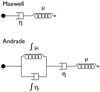 |
Fig. 1 Schematic representation of the Maxwell viscoelastic model and the Andrade anelastic model. The different models can be seen as a succession of springs (labeled as μ) and dashpots (labeled as η). The springsrepresent the elastic properties of the material while the dashpots represent its viscous properties. The Andrade model is a combination of the viscoelastic Maxwell assembly in series with an infinite number of springs and dashpots in parallel. This last part represents the memory of the material, which corresponds to the anelastic component of the assembly. |
2 Models of dissipation
We start by considering two bodies: a point mass, which we call the perturber, P, and an extended central mass, C, which is going to respond to the perturber’s gravitational potential. We refer to MP and MC as the respective masses of P and C. The radius of C will be referred to as RC. The excitation frequency will be referred to as ω, or ωlmpq, where l, m, p, q are the indices of the harmonic expansion of the potential1. We consider that the perturber is farther away than 5 × RC from the central mass and that the eccentricity is low enough that we can restrict the expansion of the tidal potential and perturbations on spherical harmonics to the l = 2 mode (e.g., Mathis & Le Poncin-Lafitte 2009; Makarov & Efroimsky 2013).
The Love number (Love 1911) quantifies the ability of a celestial body to respond to tidal forcing. It corresponds to the ratio between the additional gravitational potential induced by internal mass redistribution due to tidal deformation and the external tidal potential created by the perturber:
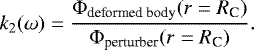 (1)
(1)
For a perfectly elastic body, k2 is a real quantity, the deformation is instantaneous, and the tidal bulges are aligned with the direction of the perturber. There is no tidal evolution in this case. However, for a real body, the response is never perfectly elastic and part of the response is dissipative, resulting in a delay or lag in the deformation. Thus, k2 becomes a complex quantity and its imaginary part quantifies the corresponding lag δ2 (Efroimsky & Makarov 2013):
 (2)
(2)
The aim here is to quantify the amplitude of k2 and the lag consistently with regard to the internal structure and rheology of various rocky planets. First, we discuss the case of a homogeneous planet and then we move on to multi-layer planets.
2.1 Dissipation of a homogeneous body
Following Efroimsky (2012b) we can express the imaginary part of the Love number as follows
![Mathematical equation: \begin{flalign}&{\textrm{Im}}[k_{2, \textrm{hom}}] = \frac{3}{2} \frac{A_2 J {\textrm{Im}}[\bar{J}(|\omega|)] \times {\textrm{sgn}}(\omega)}{\left({\textrm{Re}}[\bar{J}(|\omega|)]+A_2 J\right)^2 + \left({\textrm{Im}}[\bar{J}(|\omega|)]\right)^2},\\ &A_2 = \frac{57}{8} \frac{J^{-1}}{\pi{\mathcal{G}}\rho_{\textrm{p}}^2{R_{\textrm{p}}}^2}, \end{flalign}](/articles/aa/full_html/2020/12/aa38204-20/aa38204-20-eq3.png)
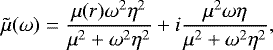
where  is the complex compliance of the material (in 1/Pa) and ω is the excitation frequency. For the Maxwell rheology model, the simplest viscoelastic model consisting of a dashpot (viscous element) and a string (elastic element) in series (Fig. 1), the complex compliance is given by:
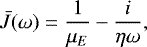 (5)
(5)
where μE = 1∕J is the (unrelaxed) elastic shear modulus, in Pa, represented by the spring in Fig. 1, and η is the shear viscosity, in Pa s, represented by the dashpot in Fig. 1. For a rheology of Andrade, the complex compliance is given by (Castillo-Rogez et al. 2011):
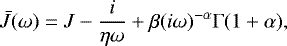 (6)
(6)
where the third term describes the transient anelastic response, which controls the behavior at forcing periods comparable to the Maxwell time, defined as τM = η∕μE = ηJ. For the sake of simplicity, we later refer to μE as μ. α is a parameter linked to the duration of the transient response in the primary creep. This parameter is commonly considered to be between 0.20 and 0.40 (Castillo-Rogez et al. 2011) based on existing laboratory constraints on olivine minerals and ices. Besides, Tobie et al. (2019) showed that a parameter value between 0.23 and 0.28 allowed us to reproduce the dissipation factor of the present-day solid Earth quite well. Then, β describes the intensity of anelastic friction in the material and is given by:
 (7)
(7)
where τA is the timescale associated to the Andrade creep, later referred as the Andrade time. The quantity β can be expressed with the dimensionless parameter ζ defined as ζ = τA∕τM :
 (8)
(8)
Castillo-Rogez et al. (2011) showed that under low stress, ζ ≈ 1. To compute the dissipation, we fix ζ = 1 but to fit the parameters of a homogeneous planet to the response of a multi-layer planet (see Sect. 3), we treat it as a free parameter.
At tidal periods that are much shorter than τM (high frequency), the response is dominated by the elastic behaviour, whereas at tidal periods that are much longer, it is dominated by viscous behaviour. Compared to the classically used Maxwell rheology, the Andrade rheology provides a more accurate description of the frequency dependency of both elastic and dissipative responses across a wide range of forcing frequencies and periods. The Maxwell rheological model provides a reasonable description of viscoelastic behavior for forcing periods near and larger than that of the Maxwell time, but it strongly underestimates viscous dissipation (or overestimates the Q factor) for forcing periods that are much smaller than the Maxwell time (e.g., Efroimsky 2012b; Tobie et al. 2019).
To summarize, calculating the tidal response of a homogeneous body of given mass and radius requires effective values of the shear modulus μ, the shear viscosity η, along with the α and ζ parameters representative of the entire planetary interior. Figure 2 shows the dependence of the imaginary part of the Love number with the excitation frequency for different values of these four parameters. Figure 2a shows that parameter α influences the behavior at high frequencies: the higher α, the steeper the slope. Figure 2b shows that changing the viscosity at constant shear modulus leads to a shift of the frequency at which the maximum dissipation occurs. The maximum dissipation occurs at a frequency which is 1∕τM = μ∕η such that increasing the viscosity leads to a frequency shift of the dissipation maximum towards the small frequencies. Figure 2c shows that the shear modulus impacts both the intensity of the maximum of dissipation and its frequency position. The higher the shear modulus (or the smaller the Maxwell Time), the higher the maximum dissipation and the higher the frequency corresponding to the maximum dissipation. Finally, changing the ratio of Andrade Time over Maxwell Time modifies the value of the maximum dissipation (see Fig. 2d) and the slope occurring around a frequency of 10−9 rad s−1. The higher ζ, the more pronounced the peak.
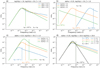 |
Fig. 2 Dissipation as a function of the excitation frequency for a homogeneous body; (a) effect of the parameter α; (b) effect of the viscosity η; (c) effect of the shear modulus μ; (d) effect of the parameter ζ. We note that the value ζ = +∞ corresponds to a Maxwell model. |
2.2 Dissipation in a multi-layer body
To calculate the distribution of tidal dissipation in a spherical multilayer body, we use the elastic formulation of spheroidal oscillation developed by Takeushi & Saito (1972), adapted to the viscoelastic case by Tobie et al. (2005), using the correspondence principle (Biot 1954), and recently adapted to multilayer solid exoplanets (Tobie et al. 2019).
Modeling the tidal response of a multi-layered interior consists of determining the displacements, stresses, and potential perturbations induced by an external potential at any point in the body by solving the equation of motions and Poisson equations with appropriate boundary conditions and by considering a given stress-strain relationship, representative of the materials that compose theplanetary interior. By assuming a spherically symmetric layered interior (i.e., with no lateral variations in material properties isallowed), the problem solutions can be separated into a radial component and an orthoradial component using the spherical harmonics basis.
Following the approach of Takeushi & Saito (1972), the spheroidal deformations of a spherically symmetric layered interior can be formulated by using six radial functions, yi, that satisfy a set of differential equations:
 (9)
(9)
The matrix Aij depends on the excitation frequency, ωlmpq, on the density profile, ρ(r), on the compressibility modulus, κE(r), and on the shear modulus, μE(r) = μ(r) in the elastic case, and on the acceleration due to gravity. The functions y1 and y3 are respectively associated to the radial and tangential displacement, while y2 and y4 are associated to the radial and tangential stresses. The fifth function, y5, is associated to the gravitational potential and y6 allows us to ensure the continuity of the gradient of the gravitational potential, defined by
![Mathematical equation: \begin{equation*}\begin{array}{ll} y_6(r, \omega_{lmpq}) &\displaystyle= \frac {\mathrm{d}y_5(r, \omega_{lmpq})}{\mathrm{d}r} - 4\pi G \rho y_1(r, \omega_{lmpq}) \\[10pt] &\displaystyle \quad+ \frac {l+1}{r} y_5(r, \omega_{lmpq}). \end{array} \end{equation*}](/articles/aa/full_html/2020/12/aa38204-20/aa38204-20-eq10.png) (10)
(10)
At the planet surface, the potential Love number of degree l is given by
 (11)
(11)
with Rp the radius of the body. Here, we only consider the degree-2 tidal potential (it is enough if the perturber is more than 5 Rp from the considered body and the eccentricity is low; e.g., Mathis & Le Poncin-Lafitte 2009; Makarov & Efroimsky 2013). In the following, for simplicity, we refer to ωlmpq as ω. For a purely elastic body, the relationship between the stress tensor and the strain tensor is determined by a Hooke’s law (e.g., Melchior 1973).
Here, we assume a viscoelastic rheology and use the correspondence principle from Biot (1954). This principle states that for the same initial condition and geometry, the formulation of the elastic problem is equivalent to the formulation of the viscoelastic problem when the rheological parameters and the previously defined radial functions are complex. This means that the relation between the strain ɛi,j and stress σi,j tensors for elastic bodies can be generalized for viscoelastic bodies as a generalized Hooke’s law in the frequency domain:
 (12)
(12)
where the tilde indicates a complex value in the frequency domain, δi,j is the Kronecker’s function,  is a complex shear modulus, and
  is a complex compressibility modulus. For a Maxwell rheological model, the complex shear modulus, which corresponds to the inverse of the complex compliance given in Eq. (5), is
 (13)
(13)
which depends on the excitation frequency, ω, but also the radial coordinate, r, via the radial dependence of the elastic shear modulus, μ(r), and the viscosity, η(r). For the Andrade rheology, in a similar manner, the complex shear modulus is just the inverse of complex compliance given in Eq. (6).
The correspondence principle is equivalent to a consideration of the equations governing the system but replacing the yi functions with their complex counterparts, ỹi, the elastic shear modulus, μ with the complex,  , the compressibility modulus, κE, with
  and the Love number of Eq. (11) with
  . The imaginary part of these quantities governs the dissipative response of the planet while the real part describes the instantaneous elastic response. The imaginary part of the complex shear modulus is controlled by the shear viscosity, η(r), whereas the complex bulk modulus depends on the bulk viscosity, ηb(r). As the bulk viscosity is poorly constrained for planetary materials (e.g., Bercovici et al. 2001), the dissipative part of
  is often neglected and only the elastic, real part is considered (e.g., Tobie et al. 2005).
In order to calculate the dissipation of a multi-layer body, we therefore need the profiles of the density, bulk modulus, shear modulus, and shear viscosity, as well as a rheological model to compute the complex shear modulus from the above-cited rheological parameters assumed in each layer. The complex compliance is computed using Eqs. (5) or (6) depending on whether a Maxwell or Andrade rheology is assumed. For the sake of simplicity, we assume the same rheological models in all internal layers. In the case of the Andrade model, we also consider the same constant parameters, α and ζ = τA∕τM = 1, for all internal layers.
We calculate the response of different bodies within this formalism for three different α parameters: 0.15, 0.25, and 0.35, which bracket the reasonable parameter space (Castillo-Rogez et al. 2011). Finally, for the profiles of the different quantities (density, compressibility modulus, shear modulus, and viscosity) we use the following internal structure model.
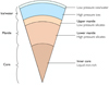 |
Fig. 3 Internal structure model. |
2.3 Internal structure model
For the planets we consider in this study (a planet of 0.5 M⊕; an Earth-like planet; two Super-Earths of 5 M⊕ and 10 M⊕; and TRAPPIST-1e), we obtain the radial profiles of the different quantities following the formalism of Sotin et al. (2007). Here, we present the main ingredients and characteristics of the internal structure model and we refer the reader to Sotin et al. (2007) for details. We also study the case of a Venus-like planet, for which we use a more specific model based on Dumoulin et al. (2017).
2.3.1 Generic model from Sotin et al. (2007)
The most generic model is composed of five layers: one layer representing the inner core, two layers for the mantle, and two layers for ices and liquid water on top. Figure 3 shows the set up.
In this model, the first and innermost layer is a liquid iron-rich core. For the sake of simplicity, no solid inner iron core is considered, as it has a minimal effect on the global tidal deformation (Dumoulin et al. 2017; Tobie et al. 2019).
The mantle is divided into two layers due to a mineralogical transformation that occurs at a pressure of about 25 GPa. Similar to the Earth’s lower mantle, the lowermost part of the silicate mantle is composed of high-pressure silicate minerals: perovskite and magnesiowüstite2. The upper mantle (third layer) is composed of low pressure silicate minerals: olivine, ortho- and clino-pyroxenes, and garnet. For ice-rich exoplanets, two additional layer are considered: a high-pressure ice layer when the pressure exceeds 2.2 GPa (fourth layer) and low-pressure ice layer or water layer (fifth layer) depending on the surface temperature. This outer layer is very thin and does not contribute significantly to the mass-radius relationship of the planet (Sotin et al. 2007). However, its physical state (liquid or solid) can significantly affect the tidal deformation and dissipation (e.g., Auclair-Desrotour et al. 2018, 2019) and, therefore, its thickness and state need to be carefully determined to correctly predict the tidal response.
Following the approach of Sotin et al. 2007, namely, a Birch-Murnagan equation of state (EoS), up to the third order in finite strain, is considered for the upper mantle and the low-pressure ice layer or water layer (layers 3 and 5), whereas a Mie-Grunëisen-Debye is employed for the iron core, the lower silicate mantle, and the high-pressure ice mantle (layers 1, 2, 4).
The elastic bulk isentropic modulus, K, is derived from the density and pressure profiles
 (14)
(14)
The shear modulus, μ, in each solid layer is then estimated from the bulk modulus and the pressure. For the silicate part, the following relationship, which reproduces the shear modulus profile in the Earth’s mantle well (Dziewonski & Anderson 1981; Stacey & Davis 2008), is used
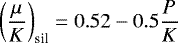 (15)
(15)
for P < 25 GPa and
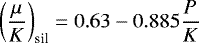 (16)
(16)
for P > 25 GPa. For pressure above 130 GPa, we neglect the phase transition to the post-perovskite and thus consider the same relationship. For the ice layers, a similar relationship constrained from existing experimental data at high pressures (Polian & Grimsditch 1983) is used:
 (17)
(17)
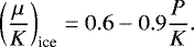
We note that μ∕K = 0.6 corresponds to a Poisson body.
The internal structure is computed from the assumed planet composition, defined using four parameters: the water mass relative to the mass of the planet, the bulk ratios of Mg/Si and Fe/Si, and the Mg content of the silicate mantle, defined as the Mg number, Mg# (the mole fraction Mg/(Mg+Fe) in the silicates). We also need to give three additional constraints: the composition of the core is fixed (here to 87% of Fe and 13% of FeS), all the water is found in layers 4 and 5 (no water incorporated in the silicates) and the mantle is chemically homogeneous. Knowing the former four parameters combined with the latter three assumptions, both the size of each layer and the mineralogical composition of the silicates mantles can be determined.
For the Earth, for instance, there is no layer 4 (no high pressure ices) and layer 5 is so thin that it does not contribute to the mass-radius relationship. The Earth-like planet we consider here is an ocean-less planet3 of Earth’s radius and mass so that layer 5 does not exist either. In this model, Earth is therefore made up of three layers, the upper mantle, the lower mantle, and the liquid core (we note that here we neglect the Earth’s small solid core as it represents only 2% of Earth’s mass). This model reproduces the Preliminary Reference Earth Model (PREM, Dziewonski & Anderson 1981) as shown in Sotin et al. (2007). For the Earth-like planet as well as the 0.5 M⊕ planet and the two super-Earths, we also vary the Fe/Si ratio compared to the Earth’s ratio. We consider three different Fe/Si contents compared to the Earth’s: 50, 100, and 150%. For a constant mass, increasing the quantity of iron leads to a denser and smaller planet. Table 1 summarizes the assumed parameters for the different planets considered in this study.
Viscous dissipation is generated in the solid layers where the viscosity and shear modulus are non-zero. The liquid core and the water ocean (when present) are assumed to be inviscid, which means that there is no viscous dissipation at all in these layers. This does not mean that in reality, no dissipation exists in this layer, for instance, due to turbulence or any liquid-solid friction at interfaces (e.g., Ogilvie 2014; Mathis 2018). Nevertheless, such processes are not considered in our viscoelastic formalism and, therefore, any dissipation is assumed to be negligible in liquid layers.
2.3.2 Specific model for Venus
We follow the work from Dumoulin et al. (2017) for the structural profiles of Venus. The mass and radius of Venus used in this model are given in Table 1. We refer to this publication for further details of the interior model for Venus. We use the temperature and pressure profiles from Steinberger et al. (2010) (hereafter, S10, cold profile) and Armann & Tackley (2012) (hereafter, AT12, hot profile).
Radial density, ρ, and seismic velocities, Vp and Vs, are computed from hydrostatic pressure, temperature, and composition using the Perple_X program (Connolly 2005) developed by James Connolly4 in the mantle and from PREM extrapolation in the metallic core (Dziewonski & Anderson 1981). The Perple_X method computes phase equilibria and uses the thermodynamics of mantle minerals developed by Stixrude & Lithgow-Bertelloni (2011).
As in the tests performed in Dumoulin et al. (2017), we use the following formula to compute the viscosity as a function of the temperature and pressure profiles:
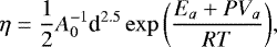 (18)
(18)
where Ea, Va, and A0 are parameters depending on the material and d is the grain size. Here, we consider dry olivine: Ea = 300 kJ mol−1, Va = 6 cm3 mol−1, and A0 = 6.08 × 10⁻¹⁹ Pa−1 s−1. We consider here a grain size d equal to 0.68 mm so that the factor  Pa s. The shear and bulk moduli are calculated from the density and the seismic velocity Vs and Vp as follows:
  and
and 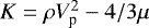 . The corresponding shear modulus and the viscosity profiles are shown in Fig. 4.
The colder profile (S10) results in a much higher viscosity and a shear modulus slightly larger than the hot profile (AT12). These two profiles can be considered as end members. Figure 4 displays the average parameter profiles for these two end-member interior models. Here and in the following sections, the averages of shear modulus and viscosity are calculated as follows (Dumoulin et al. 2017):
![Mathematical equation: \begin{equation*}\langle \mu\rangle = \exp{\left[\frac{1}{V_{\textrm{shell}}} \int_{V_{\textrm{shell}}}{\ln{\mu}\textrm{d}v}\right]}, \end{equation*}](/articles/aa/full_html/2020/12/aa38204-20/aa38204-20-eq28.png) (19)
(19)
where Vshell is the volume of the shell where viscosity and shear modulus are non-zero.
Characteristics of the planets considered in this article.
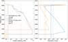 |
Fig. 4 Shear modulus and viscosity profiles for the two end-member interior models considered here. The viscosity η is calculated as in Dumoulin et al. (2017), using Eq. (18) of this work. The dotted lines represent the average of shear modulus and viscosity of the two profiles. The dashed lines correspond to the best fit of the dissipation of the multi-layer planet (see Sect. 3.2). |
3 Dissipation of multi-layer planets as a function of the excitation frequency
3.1 Earth-like planet and super-Earths
Here, we use a simple representation of Earth-like planets with three isoviscous layers and a shear modulus consistent with the PREM (as shown in Sect. 2.3.1, Fig. 5). Figure 6 shows the imaginary part of the Love number, representing the amplitude of dissipation, for an ocean-less Earth-like planet as a function of the excitation frequency for a three-layer model and two homogeneous models.
The full lines show the dissipation of the planet using the multi-layer model described in Sect. 2.2, using the profiles from Fig. 5. The dotted line corresponds to the dissipation obtained considering a homogeneous planet following Sect. 2.1, for which we assumed an averaged value for the shear modulus and the viscosity (Eq. (19)). Finally, the dashed lines correspond to the dissipation of a homogeneous planet for which we fitted the values of the shear modulus, the viscosity, and ζ = τA∕τM, in order to obtain a dissipation amplitude similar to the three-layer model.
The fits were performed using the python library, Non-Linear Least-Squares Minimization and Curve-Fitting for Python (LMFIT5). We used weights to force the fit to reproduce preferentially the amplitude and position of the dissipation maximum. We evaluate the quality of our fits by calculating the root mean square error (RMSE) as follows
 (20)
(20)
where N is the number of individual excitation frequency values we consider, Imk2,multi(ωi) is the imaginary part of the Love number we calculate using the multi-layer framework of Sect. 2.2, estimated at the excitation frequency, ωi. In addition, Im k2,fit homog(ωi) is the imaginary part of the Love number we calculate using the homogeneous model of Sect. 2.1 with the fitted parameters for shear modulus, viscosity, and ζ. In our fits, we do not treat α as a free parameter, but we use the same value as the one that was used for the different layers of the multi-layer model. This ensures that the slope at high frequencies is accurately reproduced. As Fig. 2 shows, shear modulus, viscosity, and the ζ parameter influence the amplitude (through μ) and position(through η) of the maximum of dissipation and the relative weight of the maximum over the high frequency behavior (through ζ). Table 2 shows the best-fit parameters for all planets considered here.
One result shown in Fig. 6 demonstrates that considering a homogeneous body of averaged viscosity and shear modulus leads to a non-negligible overestimation of the dissipation. If we compare the result for this averaged dissipation to the dissipation corresponding to the multi-layer body of same α (the green full line), it is more than 2.5 times higher and the difference increases with increasing frequency. The position of the dissipation maximum is also slightly shifted to the higher frequencies. These two major differences can be understood by comparing the order of magnitudes of the values of the averaged shear modulus and viscosity with the values of the fitted shear modulus and viscosity (Fig. 5), which allow us to best reproduce the multi-layer dissipation. The averaged viscosity is very close to the best fit values, while the averaged shear modulus is much higher than the best fit values. Figure 2c shows that at constant viscosity, the higher the shear modulus, the higher the peak of dissipation maximum, and the more shifted the peak to the high frequencies, keeping the low frequency slope super-imposed. Figure 6 shows that exact behavior, which means that the dissipation using a homogeneous body with average values perform fairly well for the very low frequencies and is an overestimation at frequencies higher than the one corresponding to the maximum of dissipation. We note that computing the logarithmic volume-weighted average as we did (Eq. (19)) yields a similar viscosity (~ 1022.1 Pa s) as the best fits (around 1022.2 Pa s, see Table 2), but that is not the case if we perform a linear volume-weighted average (which amounts to ~ 1023.8 Pa s) as is done in Barr et al. (2018). The higher viscosity then leads to a shift of the peak to lower frequencies (see Fig. 2b), which means that using a linear volume-weighted average leads to an underestimation of the dissipation over the whole frequency range. The viscosity varies by several orders of magnitude between the low-viscosity layers (upper mantle and bottom thermal boundary layer) and the high-viscosity ones (top boundary layer and lower mantle). The linear average of the viscosity is therefore much more representative of the high-viscosity layers. Performing a logarithmic average allows us to compute a viscosity that better represents the low-viscosity layers, without being too far from the high-viscosity ones. We believe that as viscosity is a key factor in controlling the position of the maximum of dissipation, a consideration of the low-viscosity layers is important for obtaining a better approximation of a layered media using a constant parameter. This is confirmed by the fact that the best-fitting constant viscosity is very close to the logarithmic average of the varying viscosity.
Figure 6 shows that the fit quality is better at high frequencies than at low frequencies, where we see a bump occurring around ω ≈5 × 10⁻¹³ rad s−1. This low frequency behavior is due to the fact that the lower mantle has a higher viscosity value than the upper mantle. This leads to the secondary dissipation peak, explaining the curve bump at low frequencies, around 10−14 rad s−1.
Figure 7 shows the dissipation curves but for planets with different masses (left panel) and Fe/Si ratios (right panel). The higher the mass of the planet, the lower the dissipation peak. For an Earth-like planet, the maximum is about Im k2 ≈ 0.2, while it is 0.13−0.15 for the 5 M⊕ planet and 0.11 for the 10 M⊕ planet. The higher the mass of the planet, the lower the frequency of the maximum of dissipation. We provide the best-fit values of shear modulus and viscosity for different α and Fe/Si ratios in Table 2.
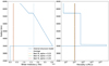 |
Fig. 5 Profiles of the shear modulus, μ, and the viscosity, η, for an Earth-like planet (with Fe/Si = 100%) in full lines. The dotted lines represent the average value of both quantities. The dashed lines represent the values obtained by fitting a homogeneous model to the dissipation response of the planet for three different values of the parameter α (see Fig. 6). |
 |
Fig. 6 Imaginary part of the Love number Imk2 as a function of the excitation frequency for an Earth-like planet (without ocean). Full lines: dissipation of a multi-layer body for three different α parameters (but α is the same for the different layers of these 3 cases). Dotted black line: dissipation of a homogeneous body for which we assumed the averaged value of the multi-layer profiles for shear modulus and viscosity (see Fig. 5). We also assumed a parameter α of 0.25 and assumed that the Maxwell Time is equal to the Andrade Time (ζ = 1). Dashed lines: best-fit dissipation of a homogeneous body for the three different α (the fitted values of shear modulus and viscosity are plotted in Fig. 5 and all fit parameters, including the ζ parameter, are listed in Table 2). |
3.2 Venus
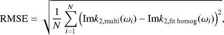
Figure 8 shows the frequency dependency of the dissipation curves for the multi-layer models of Venus (full lines), for a homogeneous body with averaged values of shear modulus and viscosity (dotted lines), and for a homogeneous body with best fit values of shear modulus and viscosity for the two end-member (cold-hot) internal structure models.
The two internal structure models lead to quite different characteristics: the “cold” profile (S10) leads to a slightly higher dissipation maximum than the “hot” profile (AT12) and the maximum dissipation occurs at shorter frequencies. This behavior can be understood from the profiles of shear modulus and viscosity for the two different structures (see Figs. 4 and 2): both quantities are higher for the cold profile than for the hot profile and this leads to a higher dissipation maximum and a maximum shifted towards shorter frequencies. Both models lead to very different dissipation values at the present-day tidal frequency of Venus (indicated with the black dashed line). The difference in the dissipation rate between the cold and hot profiles suggests that a fast-rotating early Venus would despin about ten times more quickly to its present-day rotation state for the hot interior scenario than for the cold one. This indicates that the past rotation evolution of Venus must have been rather sensitive to the thermal evolution of its mantle, calling for detailed thermal modeling is required to accurately reconstruct its rotation history (Dumoulin et al. 2018).
Considering a homogeneous body of averaged shear modulus and viscosity leads to an overestimation of the dissipation in the high frequency regime. The “hot” profile case shows a higher overestimation visible around the dissipation maximum: it is higher and slightly shifted to the higher frequencies. For the “cold” profile, the dissipation maximum is also higher but shifted to the lower frequencies. This behavior can be understood when comparing the averaged value of shear modulus and viscosity with the best-fit values (see Fig. 4) and Fig. 2. Both cases have ahigher averaged shear modulus than the best-fit value, which leads to a higher dissipation maximum, slightly shifted to the higher frequencies. For the “hot” profile, the averaged viscosity is lower than the best-fit viscosity, which contributes to shifting the dissipation maximum to even higher frequencies. For the “cold” profile, the averaged viscosity is higher than the best-fit viscosity, which shifts the dissipation maximum to lower frequencies and overcomes the shear modulus-driven shift. As for super-Earths in the previous section, the fits are not perfect. The dissipation of the multi-layer structure leads to a secondary peak in the dissipation around a frequency of 10−12 rad s−1 for the “cold” profile in blue and very close to the main peak for the “hot” profile around a frequency of 10−10 rad s−1. Considering the dissipation of a homogeneous body leads therefore here to a small underestimation of the dissipation. However, as these small differences occur at very low frequencies, their impacts on the rotation evolution should be limited. The detailed consequences in term of spin and eccentricity evolution will be investigated in a follow-up article. The fitted values of the shear modulus and viscosity can be found in Table 2 for α =0.25 (used for Fig. 8) as well as the two other values of α considered here.
Fit parameters for all planets considered here.
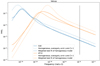 |
Fig. 8 Imaginary part of the Love number, Imk2, as a functionof the excitation frequency assuming α = 0.25. Full lines: Imk2 as calculated by the profiles of Dumoulin et al. (2017) for the two different models (hot: orange, cold: blue). Dashed lines: best fit of Imk2 for a homogeneous body. Dotted lines: obtained with the averaged values of μ and η from Fig. 4. The black vertical dashed line represents the excitation frequency of Venus (ωVenus = 2(nVenus − ΩVenus)). |
3.3 TRAPPIST-1e
The two internal structure models we use here for TRAPPIST-1e differ in their Fe/Si ratio and the consequent presence of an ice layer (see Table 1). Contrary to all the models we have discussed so far, here, we investigate the effect of the presence of an ice layer on the dissipation of a terrestrial planet.
Figure 9 also shows the profiles for two different possible internal structures of TRAPPIST-1e: a dense ice-less structure and a less dense icy structure. The ice-less structure is very similar to the one of the Earth-like planet with only three layers. We note that the value of the Fe/Si ratio has to be higher than that of the Earth in order to reproduce the observed radius (138%). The second structure has a ~ 400 km ice layer at the surface, where the three different phases of water ice (Ice I, Ice VI, Ice VII) are present. The amount of ice for this structure represents only 5% of the mass of the planet. As ice is much less dense than rocks, an even higher iron content (150%) is needed to reproduce the observed radius. The properties of these two different cases are given in Table 1.
Figure 10 shows the frequency dependence of the dissipation for these two different structures. The ice-poor structure (low iron content) is very similar to the super-Earths of Sect. 3.1 and Venus (Sect. 3.2), resulting in similar fit performance. The values of the fit are given in Table 2 for all values of α. Table 2 also shows the corresponding values of the Maxwell time for the different fits. The obtained values of the Maxwell time are orders of magnitude higher than the values of 10−2−10−1 days taken by Makarov et al. (2018) for TRAPPIST-1 planets. This means that the excitation frequency corresponding to the maximum dissipation is shifted to higher frequencies than in our work and that the maximum dissipation is also much higher in their case than in ours (see Fig. 2). We therefore expect the dissipation they calculate to be strongly overestimated compared to the one we compute in the next section (Sect. 4).
The behavior of Imk2 with frequency is very different when there is an ice-layer. Figure 10 shows two peaks occurring at different frequencies. The shorter frequency corresponds to the frequency of the rocky part of the planet (it is indeed very similar to the excitation frequency at which the maximum of the response occurs for the ice-less structure). The second peak occurring at larger frequencies corresponds to the behavior of the ice. For this specific case here, we use a constant viscosity of 1016 Pa s for the high pressure ice layer as shown on Fig. 9. This double-peaked feature makes the quality of the fit very poor.
A multilayer planet with different rocky layers can be quite well approximated by a homogeneous body with fitted values for shear modulus and viscosity but if the planet has an ice layer, then this approximation is no longer valid. By construction, the homogeneous body does not allow for the reproduction of the double-peaked feature of the dissipation6, so for icy bodies it is necessary to take into account the real multi-layer structure to correctly estimate the dissipation (or by trying the fit with a different model, e.g., Renaud & Henning 2018, but this is out of the scope of this work). The homogeneous body approximation particularly fails on a range of frequencies that depends on the viscosity of the ice layer considered.
As the viscosity of high pressure ice is relatively unknown, we tested two other values of viscosity: 1014 Pa s (close to the value of 1013 Pa s obtained from laboratory experiments given in Poirier et al. 1981) and 1018 Pa s. This range is roughly what was considered in Kalousová et al. (2018) for ice layers, which come from the two preceding articles, Sotin & Parmentier (1989) and Durham & Stern (2001).
Figure 11 shows the behavior of the dissipation response when the viscosity of the high pressure ice layer varies from 1014 to 1018 Pa s. When the viscosity of the ice layer increases, the peak linked to the dissipation in the ice layer shifts towards the shorter frequencies, which is compatible with the behavior that we would expect for a homogeneous body (see Fig. 2). The maximum of the second peak decreases slightly when the viscosity of the ice layer decreases but as the peak shifts to higher frequencies, the planet becomes significantly more dissipative for a wider range of frequencies. Given the poor quality of the fit, we do not give the fitted values of shear modulus and viscosity for the two ice-layer viscosities, 1014 and 1018 Pa s. For the following, we assume a viscosity of 1016 Pa s for the high pressure ice layer of the TRAPPIST-1 planets.
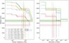 |
Fig. 9 Shear modulus and viscosity profiles for the outer TRAPPIST-1 planets for the highest iron content and, thus, the highest ice content. Here, wmf means water mass fraction. The ratio Fe/Si is given with respect to the Earth. Left panel: high pressure ices layer can be identified as the bolder part of the line. |
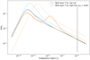 |
Fig. 10 Imaginary part of the Love number Imk2 as a function of the excitation frequency for two different internal structures of TRAPPIST-1e, assuming α = 0.25. The iron-poor structure (ice-less structure) is in blue and the iron-rich structure (with an ice layer) is in orange. Full lines: the multi-layer model. Dashed lines: the corresponding best fits of a homogeneous model. Dotted lines: homogeneous model with averaged viscosity and shear modulus. The black vertical line represents the excitation frequency ofTRAPPIST-1e, which is the orbital frequency in the following hypotheses: the rotation is synchronized, the obliquity is zero, and the eccentricity is small. |
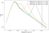 |
Fig. 11 Same as Fig. 10 but for different viscosities of the ice layer for the iron-rich internal structure for TRAPPIST-1e, assuming α = 0.25. |
4 Tidal heating of the TRAPPIST-1 planets
Here, we derive the dissipation profile within the TRAPPIST-1 planets using the multi-layer structure approach. Given the radius (Gillon et al. 2017) and estimated masses (Grimm et al. 2018) of the TRAPPIST-1 planets, the density of the planets of TRAPPIST-1 is compatible with a large amount of volatiles (Grimm et al. 2018; Dorn et al. 2018). We focus here on the outer planets of the TRAPPIST-1 systems for which the volatiles are taken to be water ice. We will study the inner planets in a follow-up article given the additional difficulty that the volatiles (which we consider being water here) in these bodies are in fluid form in the external envelope. Thus, investigating those planets would require coupling the internal structure model to a model of an steam atmosphere in runaway and in equilibrium with supercritical water fluid and, possibly, a magma ocean, which is out of the scope of this work.
In agreement with previous studies (Luger et al. 2017; Turbet et al. 2018; Grimm et al. 2018), here, we consider the planets to be in synchronous rotation, to have zero obliquities, and with small eccentricities. We consider two cases for the eccentricities of the TRAPPIST-1 planets: the ones given by the Transit-timing variation (TTV) analysis of the system in Grimm et al. (2018) and the smaller ones given in Turbet et al. (2018). The lower eccentricities given in Turbet et al. (2018) were obtained performing a N-body simulation of the system from Grimm et al. (2018) taking into account the tidal forces and torques using a CTL equilibrium tide model (Bolmont et al. 2015). The eccentricities for both cases are given in Table 3.
The planets’ masses and radii for different water mass fractions (or iron content) are given in Table 1. Figure 9 shows the radial profiles for the shear modulus and viscosity of each of the four outer TRAPPIST-1 planets, derived from the density profile estimated from the planets’ masses and radii following the same approach as in Tobie et al. (2019).
In order to calculate the tidal heating profile in the TRAPPIST-1 planets, we use Eq. (37) from Tobie et al. (2005), which is valid for synchronous planets with small eccentricities:
 (21)
(21)
where n is the orbital frequency, e is the eccentricity of the orbit, and r is the radius at which the volumetric tidal heating is estimated; Hμ represents the radial sensitivity to the shear modulus μ and is a real quantity. It depends on the radial structure of the planet and on the yi functions introduced in Sect. 2.2, as follows (from Eq. (33) of Tobie et al. 2005 for l = 2)
![Mathematical equation: \begin{equation*}\begin{array}{ll} H_{\mu} &\displaystyle = \frac{4}{3}\frac{r^2}{|\tilde\kappa + 4/3\tilde\mu|^2} \left| y_2 - \frac{\kappa - 2/3\tilde\mu}{r}(2 y_1-6 y_3)\right|^2\\[10pt] &\displaystyle\quad -\frac{4}{3} r \textrm{Re}\left\{ \frac{{\mathrm{d}} y_1^*}{{\mathrm{d}} r} (2y_1 - 6 y_3) \right\}\\[10pt] &\displaystyle\quad + \frac{1}{3} \left| 2y_1 - 6y_3\right|^2 + 6 r^2|y_4^2|/|\tilde\mu|^2 + 24 |y_3|^2. \end{array} \end{equation*}](/articles/aa/full_html/2020/12/aa38204-20/aa38204-20-eq31.png) (22)
(22)
The  in Eq. (21) is the imaginary part of the complex shear modulus given in Eq. (13). As in Tobie et al. (2005), we neglect the imaginary part of the complex incompressibility,
  thus assuming that no bulk dissipation occurs and that all dissipation is associated to shear deformation. In this formalism,
  contains all the information about the dissipation.
For comparison, we also calculate the volumetric heating of the Earth and Venus. These planets are not tidally locked but can be considered on coplanar, circular orbits. In that case, the expression of htide(r) is given by
 (23)
(23)
where Ω is the spin of the planet, M0 and a are, respectively, the mass of the Sun and the semi-major axis of Venus for the case of Venus and the mass and semi-major axis of the Moon in the case of the Earth. For the case of Venus, Ω =−2.99 × 10⁻⁷ rad s−1 (corresponding to a rotation period of − 243 day) and the excitation frequency is ω =2(n − Ω) = 1.24 × 10⁻⁶ rad s−1 (excitation period of ~56 day). For Earth, Ω =7.27 × 10⁻⁵ rad s−1 and the excitation frequency is ω =−1.41 × 10⁻⁴ rad s−1 (period of ~− 0.5 day).
Figure 12 shows the tidal heating profiles for the outer planets of TRAPPIST-1 for the different hypotheses in eccentricity and iron content, as well as the tidal heating profile of the rocky part of the Earth (black line) and of Venus for both “cold” (full grey line) and “hot” (dashed grey line) profiles. Panel a of Fig. 12 shows the profiles for the eccentricities of Grimm et al. (2018) and panel b shows the profiles for the eccentricities of Turbet et al. (2018). Within a given layer, the volumetric dissipation increases with depth, with huge variations between layers. The high pressure ice layer is the one which is responsible for the highest tidal heating, as this layer has a much lower viscosity (η = 1016 Pa s) than the mantle (η > 1021 Pa s). For all planets, we obtained on enhancement of tidal dissipation at the transition between the silicate mantle and the high-pressure ice mantle. We observe also that the enhancement of dissipation in the high pressure mantle is more pronounced with increasing ice fraction. For planet TRAPPIST-1g, which is the planet with the largest ice fraction, the tidal heating increases by about two order of magnitudes at the rock-ice interface.
One of the most striking result is that planet f dissipates more energy than the closer-in planet e. This is due to the fact that its eccentricity is about twice as high as the eccentricity of planet e (see Table 3) and the fact that planet f has a much thicker ice mantle and a slightly larger radius than planet e, which is the densest of the four outer TRAPPIST-1 planets.
The change of tidal heating with depth is mainly controlled by the behavior of the quantity  . The transition between the rock mantle and the high-pressure ice layer is characterized by a drop in shear modulus μ. The reduction of shear modulus in the high-pressure ice mantle relative to the rock mantle leads to an abrupt increase in tidal flexing, resulting in an enhancement of shear deformation, described by the sensitivity parameter to shear deformation, Hμ. Both quantities Hμ and
  increase towards the interior of the planet in the high pressure ice layer and are maximized at the interface.
  depends on the quantities ηω vs. μ2. In our model, the viscosity η of each layer is constant, while the shear modulus of the high pressure ices layer increases towards the interior of the planet (see Fig. 9, the bolder part of the curve corresponds to the high pressure ices layer). Consequently, if the quantity ηω is much higher than μ2, then
  varies as μ2, which is the case for most of the layers of planet g and of all the other planets.
The differences in the composition of the planets do not entail a radical difference in the dissipated energy, but they are, nonetheless, statistically significant. Due to fact that most of the dissipation occurs in the high-pressure ice layer, the planets with the higher iron content, which also have a higher quantity of water in order to fit the M–R relationship, have a higher dissipation. The difference between the iron poor and iron rich compositions is the lowest for planet e, where the total energy dissipated differs by about 15%. This difference is of about 35% for planets f and g and reaches 36% for planet g.
Table 3 summarizes the averaged quantities: total energy dissipated (called “dissipation” in the table) and the resulting tidal heat flux at the surface of the planet for the multi-layer planet model and the homogeneous model (using the averaged shear modulus and viscosity displayed in Fig. 9). For comparison, we calculate that the corresponding tidal dissipation in the solid Earth is 0.1 TW (which corresponds to a flux of ~ 2 × 10⁻⁴ W m−2), which is similar to the dissipation in TRAPPIST-1g. This shows that for the Earth tidal heating is a tiny fraction of the total budget. Indeed, the total heat of the Earth (due to radiogenic power and secular cooling) is estimated between 44 and 46 TW (Pollack et al. 1993; Jaupart et al. 2007). The total power produced by radiogenic heat sources in the Earth’s mantle and crust is estimated between 17 and 23 TW (Jaupart et al. 2007). We also calculated the global tidal dissipation for Venus to be ~ 3 × 10⁻⁴ TW (corresponding to a flux of ~ 6 × 10⁻⁷ W m−2) for the “cold” profile and about ten times higher for the hot profile with a dissipation of ~ 3 × 10⁻³ TW. Similarly, Io’s total dissipation is estimated from both thermal emission data (Spencer et al. 2000; Veeder et al. 2004; Rathbun et al. 2004) and astrometric data (Lainey et al. 2009) to range between 60 and 170 TW according to observational uncertainties, with average values reported by various studies of the order of 100 TW.
We find a dissipation of ~10 TW for TRAPPIST-1e, which is 4 orders of magnitude lower than the value obtained in Table 2 of Makarov et al. (2018). The dissipation we find for a homogeneous planet with averaged shear modulus and viscosity is about 3 orders of magnitude higher than for the multi-layer model. It is therefore closer to the estimates obtained by Makarov et al. (2018). However, they have a very different approach: they are computing the maximum tidal heating rate for a homogeneous planet and a Maxwell rheology (maximized by an unphysically small Maxwell time <1 day), whereas we are calculating the heating rate for rheological parameters consistent with present-day knowledge on high-pressure ices and rocks and realistic internal structure models. Figure 11 shows that the excitation frequency of TRAPPIST-1e in our model is far from the frequency corresponding to the maximum dissipation.
For planets g and h, the total tidal power remains much smaller that the endogenic power of the Earth, indicating that it will have a negligible impact on the thermal evolution of these planets. For planets e and f, it becomes comparable to the present-day radiogenic power of the Earth. As these two planets have a rock mass estimated at about 0.7–0.8 M⊕ (Table 1) and are likely older than the Earth (system age estimated as 7.6 ± 2.2 Gyr, Burgasser & Mamajek 2017), the radiogenic power is likely smaller than 10 TW, making tidal heating the main heat source in these planets. Moreover, the fact that the tidal energy is concentrated in the high-pressure ice layer may have major impacts on their internal dynamics. As it has been proposed for large icy moons such as Titan and Ganymede (Choblet et al. 2017; Kalousová et al. 2018), heat transfer in this high-pressure ice mantle may be controlled by ice melting and meltwater transport. The occurence of strong tidal dissipation in these icy mantles would likely promote melting, especially at the rock-ice interface due to enhanced tidal dissipation. In particular, in planet f, the volumetric dissipation rate at the base of the icy mantle is above 10−7 W m−3, which exceeds, by more than one order of magnitude, the volumetric heating rate by radiogenic elements in the Earth. This localized heat source will increase the occurrence of ice melting and the possibility of water-rock interactions at the rock-ice interface in these planets, favoring the extraction and transport of nutriments from the rock mantle to the surface. These may have significant implications for the habitability of such water-rich exoplanets (Noack et al. 2016, 2017).
We obtain fluxes about two times lower than those estimated in Barr et al. (2018) for planets e and f. The authors consider multi-layer planets, but they do not take into account the interior layering to compute tidal dissipation. For each planet, they assume constant shear modulus and viscosity for the different layers, then compute volume-weighted averaged shear modulus and viscosity to finally compute the dissipation using the formulation for a homogeneous planet. This method is different to what we perform to calculate the dissipation of a homogeneous body using the averaged shear modulus and viscosity (see Eq. (5)). We show in Figs. 6 and 8 that performing this averaging and using the homogeneous body framework leads to a serious overestimation of the dissipation. As explained inSect. 3, this overestimation is even greater if we compute the dissipation from the linear volume-weighted average of the shear modulus and viscosity as in Barr et al. (2018). Indeed, due to the fact that the viscosity varies by several orders of magnitude, a linear averaging of the viscosity gives too much weight to the outer highly-viscous layer and does not allow us to take into account the impact of the low viscosity layers on the dissipation. However, we cannot strictly compare our estimates with the findings cited above as their study takes into account the dependence of viscosity on temperature. We will investigate this aspect further in a follow-up study.
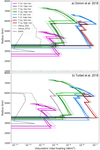 |
Fig. 12 Tidal heating profile of the outer TRAPPIST-1 planets for different eccentricities sets. Top panel: eccentricities coming from the TTV analysis of Grimm et al. (2018), tidal heating profile computed using the median eccentricity (thick line), and the standard deviation (thin lines) of the eccentricity. Bottom panel: eccentricities coming from N-body simulations with tides presented in Turbet et al. (2018). For comparison, the heating profiles of the solid Earth (black line) and Venus (grey lines: full and dashed for the “cold” and “hot” profiles respectively) are added. |
Range of possible eccentricities for the four outer planets of TRAPPIST-1 from Grimm et al. (2018), the corresponding dissipated energy and tidal heat fluxes for the low iron scenario for a multi-layer planet and for the homogeneous model with averaged values for shear modulus and viscosity from Fig. 9 (see Table 1 for the parameters of the planets).
5 Conclusions
In this work, we compute the frequency dependence of various multi-layer planetary bodies, namely: a planet of 0.5 M⊕; an Earth-like planet; two Super-Earths of 5 M⊕ and 10 M⊕; and TRAPPIST-1e. We compare it to the dissipation of homogeneous models using volume-averaged values of shear modulus and viscosity and found that doing so leads to a huge overestimation of the dissipation at all frequencies. It is, therefore, crucial to calculate the dissipation consistently using a formalism that takes into account the mechanical properties of each internal layer and consistently solves for the mechanical coupling between each internal layer when they are subject to tidal forces, for instance, the elastic formalism proposed by Takeushi & Saito (1972), which can be extended to the viscoelastic case (Tobie et al. 2005).
While considering averaged values for shear modulus and viscosity does not allow us to reproduce the dissipation of the multi-layer planet in a satisfactory way, the global dissipation and global tidal parameters (k2, Q) can be reasonably approximated by deriving the appropriate parameters, simplifying their implementation in orbital dynamics codes. By using computation results obtained for multi-layered planets, we derived the parameters for a equivalent homogeneous planet that best fits the multi-layered planet results.
The fitting procedure provides a reasonable approximation for rocky planets but remains poor for ice-rich planets. The presence of an ice layer leads to a second dissipation peak for higher frequencies than the peak corresponding to a rocky composition. The frequency of the second peak corresponding to the ice layer depends on the poorly constrained viscosity of the ice. Increasing the viscosity of the ice leads to a shift of the peak towards the shorter frequencies, where it blends with the peak corresponding to a rocky composition (of higher averaged viscosity). This double peak feature cannot be reproduced by a homogeneous planet model, so for icy planets, the full multi-layer model must be used to compute the dissipation consistently.
Using the multi-layer planet framework, we also computed the profiles of tidal heating within the outer planets of TRAPPIST-1. We find similar values as in Turbet et al. (2018), who applied a constant time lag model. We also compare our results with Barr et al. (2018), who consider the dissipation rate predicted from homogeneous interior formulation to assess the dissipation in a multi-layer planets. As we show in the present study, such an approach, based on volume-averaged shear modulus and viscosity, strongly overestimates the global dissipation rate. A certain limitation in our approach is that for simplicity, we assume constant viscosity with depth in each internal layer and we do not take into account the coupling with surface temperature-pressure conditions (e.g., Bower et al. 2019) or the thermal evolution of the interior (Barr et al. 2018). As shown in the case of Venus (Dumoulin et al. 2017), pressure- and temperature-dependent viscosity may have a significant impact on the prediction of tidal dissipation. Furthermore, we do not account for the presence of surface melts (magma ocean, water ocean) in our model, which is the reason we restricted our study to the outer planets of TRAPPIST-1. These aspects will be treated in follow-up studies.
Acknowledgements
The authors would like to thank the referee, Joseph Renaud, for his constructive comments. This work has been carried out within the framework of the NCCR PlanetS supported by the Swiss National Science Foundation. S.M. and E.B. acknowledge funding by the European Research Council through ERC grant SPIRE 647383 and by the CNES PLATO grant at CEA/DAp. This research has made use of NASA’s Astrophysics Data System.
References
- Alexander, M. E. 1973, Ap&SS, 23, 459 [NASA ADS] [CrossRef] [Google Scholar]
- Andrade, E. N. D. C. 1910, Proc. R. Soc. London Ser. A, 84, 1 [NASA ADS] [CrossRef] [Google Scholar]
- Anglada-Escudé, G., Amado, P. J., Barnes, J., et al. 2016, Nature, 536, 437 [NASA ADS] [CrossRef] [PubMed] [Google Scholar]
- Armann, M., & Tackley, P. J. 2012, J. Geophys. Res. Planets, 117, E12003 [CrossRef] [Google Scholar]
- Auclair Desrotour, P., Mathis, S., & Le Poncin-Lafitte, C. 2015, A&A, 581, A118 [NASA ADS] [CrossRef] [EDP Sciences] [Google Scholar]
- Auclair-Desrotour, P., Laskar, J., Mathis, S., & Correia, A. C. M. 2017a, A&A, 603, A108 [NASA ADS] [CrossRef] [EDP Sciences] [Google Scholar]
- Auclair-Desrotour, P., Laskar, J., & Mathis, S. 2017b, A&A, 603, A107 [NASA ADS] [CrossRef] [EDP Sciences] [Google Scholar]
- Auclair-Desrotour, P., Mathis, S., Laskar, J., & Leconte, J. 2018, A&A, 615, A23 [EDP Sciences] [Google Scholar]
- Auclair-Desrotour, P., Leconte, J., Bolmont, E., & Mathis, S. 2019, A&A, 629, A132 [NASA ADS] [CrossRef] [EDP Sciences] [Google Scholar]
- Barr, A. C., Dobos, V., & Kiss, L. L. 2018, A&A, 613, A37 [NASA ADS] [CrossRef] [EDP Sciences] [Google Scholar]
- Bercovici, D., Ricard, Y., & Schubert, G. 2001, J. Geophys. Res., 106, 8887 [NASA ADS] [CrossRef] [Google Scholar]
- Biot, M. A. 1954, J. Appl. Phys., 25, 1385 [NASA ADS] [CrossRef] [Google Scholar]
- Bolmont, E. 2018, Habitability in Brown Dwarf Systems (Berlin: Springer Nature), 62 [Google Scholar]
- Bolmont, E., Selsis, F., Raymond, S. N., et al. 2013, A&A, 556, A17 [NASA ADS] [CrossRef] [EDP Sciences] [Google Scholar]
- Bolmont, E., Raymond, S. N., Leconte, J., Hersant, F., & Correia, A. C. M. 2015, A&A, 583, A116 [NASA ADS] [CrossRef] [EDP Sciences] [Google Scholar]
- Boué, G., Correia, A. C. M., & Laskar, J. 2016, Celest. Mech. Dyn. Astron., 126, 31 [CrossRef] [Google Scholar]
- Bower, D. J., Kitzmann, D., Wolf, A. S., et al. 2019, A&A, 631, A103 [CrossRef] [EDP Sciences] [Google Scholar]
- Burgasser, A. J., & Mamajek, E. E. 2017, ApJ, 845, 110 [NASA ADS] [CrossRef] [Google Scholar]
- Castillo-Rogez, J. C., Efroimsky, M., & Lainey, V. 2011, J. Geophys. Res. Planets, 116, E09008 [NASA ADS] [CrossRef] [Google Scholar]
- Caswell, T. E., Cooper, R. F., & Goldsby, D. L. 2015, Geophys. Res. Lett., 42, 6261 [CrossRef] [Google Scholar]
- Choblet, G., Tobie, G., Sotin, C., Kalousová, K., & Grasset, O. 2017, Icarus, 285, 252 [CrossRef] [Google Scholar]
- Connolly, J. A. D. 2005, Earth Planet. Sci. Lett., 236, 524 [NASA ADS] [CrossRef] [Google Scholar]
- Correia, A. C. M., & Laskar, J. 2001, Nature, 411, 767 [NASA ADS] [CrossRef] [PubMed] [Google Scholar]
- Correia, A. C. M., Boué, G., Laskar, J., & Rodríguez, A. 2014, A&A, 571, A50 [NASA ADS] [CrossRef] [EDP Sciences] [Google Scholar]
- Delrez, L., Gillon, M., Triaud, A. H. M. J., et al. 2018, MNRAS, 475, 3577 [NASA ADS] [CrossRef] [Google Scholar]
- Dobrovolskis, A. R., & Ingersoll, A. P. 1980, Icarus, 41, 1 [NASA ADS] [CrossRef] [Google Scholar]
- Dorn, C., Mosegaard, K., Grimm, S. L., & Alibert, Y. 2018, ApJ, 865, 20 [NASA ADS] [CrossRef] [Google Scholar]
- Dumoulin, C., Tobie, G., Verhoeven, O., Rosenblatt, P., & Rambaux, N. 2017, J. Geophys. Res. Planets, 122, 1338 [CrossRef] [Google Scholar]
- Dumoulin, C., Bolmont, E., Tobie, G., et al. 2018, Eur. Planet. Sci. Congress, EPSC2018–856 [Google Scholar]
- Durham, W. B., & Stern, L. A. 2001, Ann. Rev. Earth Planet. Sci., 29, 295 [NASA ADS] [CrossRef] [Google Scholar]
- Dziewonski, A. M., & Anderson, D. L. 1981, Phys. Earth Planet. Inter., 25, 297 [NASA ADS] [CrossRef] [Google Scholar]
- Efroimsky, M. 2012a, Celest. Mech. Dyn. Astron., 112, 283 [NASA ADS] [CrossRef] [Google Scholar]
- Efroimsky, M. 2012b, ApJ, 746, 150 [NASA ADS] [CrossRef] [Google Scholar]
- Efroimsky, M., & Lainey, V. 2007, J. Geophys. Res. Planets, 112, E12003 [NASA ADS] [CrossRef] [Google Scholar]
- Efroimsky, M., & Makarov, V. V. 2013, ApJ, 764, 26 [NASA ADS] [CrossRef] [Google Scholar]
- Egbert, G. D., & Ray, R. D. 2000, Nature, 405, 775 [NASA ADS] [CrossRef] [Google Scholar]
- Eggleton, P. P., Kiseleva, L. G., & Hut, P. 1998, ApJ, 499, 853 [NASA ADS] [CrossRef] [Google Scholar]
- Frouard, J., Quillen, A. C., Efroimsky, M., & Giannella, D. 2016, MNRAS, 458, 2890 [CrossRef] [Google Scholar]
- Gillon, M., Jehin, E., Lederer, S. M., et al. 2016, Nature, 533, 221 [NASA ADS] [CrossRef] [PubMed] [Google Scholar]
- Gillon, M., Triaud, A. H. M. J., Demory, B.-O., et al. 2017, Nature, 542, 456 [NASA ADS] [CrossRef] [PubMed] [Google Scholar]
- Goldreich, P., & Soter, S. 1966, Icarus, 5, 375 [Google Scholar]
- Grimm, S. L., Demory, B.-O., Gillon, M., et al. 2018, A&A, 613, A68 [NASA ADS] [CrossRef] [EDP Sciences] [Google Scholar]
- Henning, W. G., & Hurford, T. 2014, ApJ, 789, 30 [NASA ADS] [CrossRef] [Google Scholar]
- Henning, W. G., O’Connell, R. J., & Sasselov, D. D. 2009, ApJ, 707, 1000 [NASA ADS] [CrossRef] [Google Scholar]
- Hut, P. 1980, A&A, 92, 167 [NASA ADS] [Google Scholar]
- Hut, P. 1981, A&A, 99, 126 [NASA ADS] [Google Scholar]
- Ingersoll, A. P., & Dobrovolskis, A. R. 1978, Nature, 275, 37 [NASA ADS] [CrossRef] [Google Scholar]
- Jackson, I., Faul, U. H., Fitz Gerald, J. D., & Tan, B. H. 2004, J. Geophys. Res. Solid Earth, 109, B06201 [CrossRef] [Google Scholar]
- Jaupart, C., Labrosse, S., & Mareschal, J. 2007, Treat. Geophys., 7, 223 [Google Scholar]
- Kalousová, K., Sotin, C., Choblet, G., Tobie, G., & Grasset, O. 2018, Icarus, 299, 133 [CrossRef] [Google Scholar]
- Lainey, V., Arlot, J.-E., Karatekin, Ö., & van Hoolst, T. 2009, Nature, 459, 957 [NASA ADS] [CrossRef] [PubMed] [Google Scholar]
- Lambeck, K. 1977, Phil. Trans. R. Soc. London Ser. A, 287, 545 [NASA ADS] [CrossRef] [Google Scholar]
- Laskar, J., Joutel, F., & Boudin, F. 1993, A&A, 270, 522 [NASA ADS] [Google Scholar]
- Leconte, J., Wu, H., Menou, K., & Murray, N. 2015, Science, 347, 632 [NASA ADS] [CrossRef] [Google Scholar]
- Love, A. E. H. 1911, Some Problems of Geodynamics (Cambridge: Cambridge University Press) [Google Scholar]
- Luger, R., Sestovic, M., Kruse, E., et al. 2017, Nat. Astron., 1, 0129 [Google Scholar]
- Makarov, V. V., & Efroimsky, M. 2013, ApJ, 764, 27 [NASA ADS] [CrossRef] [Google Scholar]
- Makarov, V. V., Berghea, C. T., & Efroimsky, M. 2018, ApJ, 857, 142 [NASA ADS] [CrossRef] [Google Scholar]
- Mathis, S. 2018, Handbook of Exoplanets (Cham: Springer), 24 [Google Scholar]
- Mathis, S., & Le Poncin-Lafitte, C. 2009, A&A, 497, 889 [NASA ADS] [CrossRef] [EDP Sciences] [Google Scholar]
- McCarthy, C., & Castillo-Rogez, J. C. 2013, Planetary Ices Attenuation Properties, eds. M. S. Gudipati, & J. Castillo-Rogez, Astrophys. Space Sci. Lib., 356, 183 [CrossRef] [Google Scholar]
- Melchior, P. 1973, Physique et dynamique planétaires. Géodynamique, 4 [Google Scholar]
- Mignard, F. 1979, Moon Planets, 20, 301 [NASA ADS] [CrossRef] [Google Scholar]
- Noack, L., Höning, D., Rivoldini, A., et al. 2016, Icarus, 277, 215 [NASA ADS] [CrossRef] [Google Scholar]
- Noack, L., Snellen, I., & Rauer, H. 2017, Space Sci. Rev., 212, 877 [NASA ADS] [CrossRef] [Google Scholar]
- Noyelles, B., Frouard, J., Makarov, V. V., & Efroimsky, M. 2014, Icarus, 241, 26 [NASA ADS] [CrossRef] [Google Scholar]
- Ogilvie, G. I. 2014, ARA&A, 52, 171 [Google Scholar]
- Ogilvie, G. I., & Lin, D. N. C. 2004, ApJ, 610, 477 [NASA ADS] [CrossRef] [Google Scholar]
- Poirier, J. P., Sotin, C., & Peyronneau, J. 1981, Nature, 292, 225 [CrossRef] [Google Scholar]
- Polian, A., & Grimsditch, M. 1983, Phys. Rev. B, 27, 6409 [NASA ADS] [CrossRef] [Google Scholar]
- Pollack, H. N., Hurter, S. J., & Johnson, J. R. 1993, Rev. Geophys., 31, 267 [NASA ADS] [CrossRef] [Google Scholar]
- Rathbun, J. A., Spencer, J. R., Tamppari, L. K., et al. 2004, Icarus, 169, 127 [NASA ADS] [CrossRef] [Google Scholar]
- Renaud, J. P., & Henning, W. G. 2018, ApJ, 857, 98 [NASA ADS] [CrossRef] [Google Scholar]
- Sotin, C., & Parmentier, E. M. 1989, Phys. Earth Planet. Inter., 55, 10 [CrossRef] [Google Scholar]
- Sotin, C., Grasset, O., & Mocquet, A. 2007, Icarus, 191, 337 [NASA ADS] [CrossRef] [Google Scholar]
- Spencer, J. R., Rathbun, J. A., Travis, L. D., et al. 2000, Science, 288, 1198 [NASA ADS] [CrossRef] [PubMed] [Google Scholar]
- Stacey, F. D., & Davis, P. M. 2008, Physics of the Earth (Cambridge: Cambridge University Press) [CrossRef] [Google Scholar]
- Steinberger, B., Werner, S. C., & Torsvik, T. H. 2010, Icarus, 207, 564 [CrossRef] [Google Scholar]
- Stixrude, L., & Lithgow-Bertelloni, C. 2011, Geophys. J. Int., 184, 1180 [NASA ADS] [CrossRef] [Google Scholar]
- Sundberg, M., & Cooper, R. F. 2010, Philos. Mag., 90, 2817 [Google Scholar]
- Takeushi, H., & Saito, M. 1972, Methods Comput. Phys., 1, 217 [Google Scholar]
- Tobie, G., Mocquet, A., & Sotin, C. 2005, Icarus, 177, 534 [NASA ADS] [CrossRef] [Google Scholar]
- Tobie, G., Grasset, O., Dumoulin, C., & Mocquet, A. 2019, A&A, 630, A70 [CrossRef] [EDP Sciences] [Google Scholar]
- Turbet, M., Bolmont, E., Leconte, J., et al. 2018, A&A, 612, A86 [CrossRef] [EDP Sciences] [Google Scholar]
- Veeder, G. J., Matson, D. L., Johnson, T. V., Davies, A. G., & Blaney, D. L. 2004, Icarus, 169, 264 [NASA ADS] [CrossRef] [Google Scholar]
- Walterová, M., & Běhounková, M. 2017, Celest. Mech. Dyn. Astron., 129, 235 [CrossRef] [Google Scholar]
- Webb, S., & Jackson, I. 2003, Phys. Chem. Minerals, 30, 157 [CrossRef] [Google Scholar]
- Zanazzi, J. J.,& Triaud, A. H. M. J. 2019, Icarus, 325, 55 [NASA ADS] [CrossRef] [Google Scholar]
The generic form of the excitation is: ωlmpq = (l − 2p + q)n − mΩ, where n is the mean motion of the planet and Ω is its spin. For a circular coplanar orbit, ω = ω2200 = 2(n − Ω).
Note: we do not take into account here the post-perovskite phase (high-pressure phase of perovskite). While taking into account this phase should not change the mass-radius relationship of the planets, it could have an impact on the tidal heating through the viscosity and shear modulus.
We note that Earth’s ocean are responsible for most of the dissipation (via the complex interaction of the oceans with the rocky surface; see Lambeck 1977; Egbert & Ray 2000).
It uses many of the optimization methods of scipy.optimize, see https://lmfit.github.io/lmfit-py/index.html
Note: adding two homogeneous models with different weights to reproduce the two peaks does not work either in so far as it does not reproduce the high frequency behavior.
All Tables
Range of possible eccentricities for the four outer planets of TRAPPIST-1 from Grimm et al. (2018), the corresponding dissipated energy and tidal heat fluxes for the low iron scenario for a multi-layer planet and for the homogeneous model with averaged values for shear modulus and viscosity from Fig. 9 (see Table 1 for the parameters of the planets).
All Figures
|
Fig. 1 Schematic representation of the Maxwell viscoelastic model and the Andrade anelastic model. The different models can be seen as a succession of springs (labeled as μ) and dashpots (labeled as η). The springsrepresent the elastic properties of the material while the dashpots represent its viscous properties. The Andrade model is a combination of the viscoelastic Maxwell assembly in series with an infinite number of springs and dashpots in parallel. This last part represents the memory of the material, which corresponds to the anelastic component of the assembly. |
| In the text | |
|
Fig. 2 Dissipation as a function of the excitation frequency for a homogeneous body; (a) effect of the parameter α; (b) effect of the viscosity η; (c) effect of the shear modulus μ; (d) effect of the parameter ζ. We note that the value ζ = +∞ corresponds to a Maxwell model. |
| In the text | |
|
Fig. 3 Internal structure model. |
| In the text | |
|
Fig. 4 Shear modulus and viscosity profiles for the two end-member interior models considered here. The viscosity η is calculated as in Dumoulin et al. (2017), using Eq. (18) of this work. The dotted lines represent the average of shear modulus and viscosity of the two profiles. The dashed lines correspond to the best fit of the dissipation of the multi-layer planet (see Sect. 3.2). |
| In the text | |
|
Fig. 5 Profiles of the shear modulus, μ, and the viscosity, η, for an Earth-like planet (with Fe/Si = 100%) in full lines. The dotted lines represent the average value of both quantities. The dashed lines represent the values obtained by fitting a homogeneous model to the dissipation response of the planet for three different values of the parameter α (see Fig. 6). |
| In the text | |
|
Fig. 6 Imaginary part of the Love number Imk2 as a function of the excitation frequency for an Earth-like planet (without ocean). Full lines: dissipation of a multi-layer body for three different α parameters (but α is the same for the different layers of these 3 cases). Dotted black line: dissipation of a homogeneous body for which we assumed the averaged value of the multi-layer profiles for shear modulus and viscosity (see Fig. 5). We also assumed a parameter α of 0.25 and assumed that the Maxwell Time is equal to the Andrade Time (ζ = 1). Dashed lines: best-fit dissipation of a homogeneous body for the three different α (the fitted values of shear modulus and viscosity are plotted in Fig. 5 and all fit parameters, including the ζ parameter, are listed in Table 2). |
| In the text | |
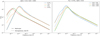 |
Fig. 7 As in Fig. 6 but for different planetary masses and different Fe/Si ratios. |
| In the text | |
|
Fig. 8 Imaginary part of the Love number, Imk2, as a functionof the excitation frequency assuming α = 0.25. Full lines: Imk2 as calculated by the profiles of Dumoulin et al. (2017) for the two different models (hot: orange, cold: blue). Dashed lines: best fit of Imk2 for a homogeneous body. Dotted lines: obtained with the averaged values of μ and η from Fig. 4. The black vertical dashed line represents the excitation frequency of Venus (ωVenus = 2(nVenus − ΩVenus)). |
| In the text | |
|
Fig. 9 Shear modulus and viscosity profiles for the outer TRAPPIST-1 planets for the highest iron content and, thus, the highest ice content. Here, wmf means water mass fraction. The ratio Fe/Si is given with respect to the Earth. Left panel: high pressure ices layer can be identified as the bolder part of the line. |
| In the text | |
|
Fig. 10 Imaginary part of the Love number Imk2 as a function of the excitation frequency for two different internal structures of TRAPPIST-1e, assuming α = 0.25. The iron-poor structure (ice-less structure) is in blue and the iron-rich structure (with an ice layer) is in orange. Full lines: the multi-layer model. Dashed lines: the corresponding best fits of a homogeneous model. Dotted lines: homogeneous model with averaged viscosity and shear modulus. The black vertical line represents the excitation frequency ofTRAPPIST-1e, which is the orbital frequency in the following hypotheses: the rotation is synchronized, the obliquity is zero, and the eccentricity is small. |
| In the text | |
|
Fig. 11 Same as Fig. 10 but for different viscosities of the ice layer for the iron-rich internal structure for TRAPPIST-1e, assuming α = 0.25. |
| In the text | |
|
Fig. 12 Tidal heating profile of the outer TRAPPIST-1 planets for different eccentricities sets. Top panel: eccentricities coming from the TTV analysis of Grimm et al. (2018), tidal heating profile computed using the median eccentricity (thick line), and the standard deviation (thin lines) of the eccentricity. Bottom panel: eccentricities coming from N-body simulations with tides presented in Turbet et al. (2018). For comparison, the heating profiles of the solid Earth (black line) and Venus (grey lines: full and dashed for the “cold” and “hot” profiles respectively) are added. |
| In the text | |
Current usage metrics show cumulative count of Article Views (full-text article views including HTML views, PDF and ePub downloads, according to the available data) and Abstracts Views on Vision4Press platform.
Data correspond to usage on the plateform after 2015. The current usage metrics is available 48-96 hours after online publication and is updated daily on week days.
Initial download of the metrics may take a while.