| Issue |
A&A
Volume 691, November 2024
|
|
|---|---|---|
| Article Number | L3 | |
| Number of page(s) | 7 | |
| Section | Letters to the Editor | |
| DOI | https://doi.org/10.1051/0004-6361/202451532 | |
| Published online | 25 October 2024 | |
Letter to the Editor
Drifts of the substellar points of the TRAPPIST-1 planets
1
Observatoire de Genève, Université de Genève, 51 Chemin Pegasi, 1290 Sauverny, Switzerland
2
Centre Vie dans l’Univers, Faculté des sciences, Université de Genève, Quai Ernest-Ansermet 30, 1211 Genève 4, Switzerland
3
Kapteyn Astronomical Institute, University of Groningen, Groningen, The Netherlands
4
Laboratoire de Planétologie et Géosciences, UMR-CNRS 6112, Nantes Université, 2 rue de la Houssinière, BP 92208, 44322 Nantes Cedex 3, France
5
naXys, Department of Mathematics, University of Namur, 61 Rue de Bruxelles, 5000 Namur, Belgium
6
Harvard-Smithsonian Center for Astrophysics, 60 Garden Street, Cambridge, MA, 02138
USA
7
Laboratoire de Recherche en Neuroimagerie, University Hospital (CHUV), Lausanne, Switzerland
⋆ Corresponding authors; alexandre.revol@unige.ch, emeline.bolmont@unige.ch
Received:
16
July
2024
Accepted:
18
September
2024
Accurate modeling of tidal interactions is crucial for interpreting recent JWST observations of the thermal emissions of TRAPPIST-1 b and c and for characterizing the surface conditions and potential habitability of the other planets in the system. Indeed, the rotation state of the planets, driven by tidal forces, significantly influences the heat redistribution regime. Due to their proximity to their host star and the estimated age of the system, the TRAPPIST-1 planets are commonly assumed to be in a synchronization state. In this work, we present the recent implementation of the co-planar tidal torque and forces equations within the formalism of Kaula in the N-body code Posidonius. This enables us to explore the hypothesis of synchronization using a tidal model well suited to rocky planets. We studied the rotational state of each planet by taking into account their multi-layer internal structure computed with the code Burnman. Our simulations show that the TRAPPIST-1 planets are not perfectly synchronized but oscillate around the synchronization state. Planet-planet interactions lead to strong variations on the mean motion and tides fail to keep the spin synchronized with respect to the mean motion. As a result, the substellar point of each planet experiences short oscillations and long-timescale drifts that lead the planets to achieve a synodic day with periods varying from 55 years to 290 years depending on the planet.
Key words: planets and satellites: dynamical evolution and stability / planets and satellites: terrestrial planets / planet-star interactions
© The Authors 2024
 Open Access article, published by EDP Sciences, under the terms of the Creative Commons Attribution License (https://creativecommons.org/licenses/by/4.0), which permits unrestricted use, distribution, and reproduction in any medium, provided the original work is properly cited.
This article is published in open access under the Subscribe to Open model. Subscribe to A&A to support open access publication.
1. Introduction
The first results of JWST thermal emission observations of the rocky exoplanets of the TRAPPIST-1 system (Gillon et al. 2017) have been published; they focus on the characterization of the atmosphere of TRAPPIST-1 b (Greene et al. 2023; Ih et al. 2023) and TRAPPIST-1 c (Zieba et al. 2023; Lincowski et al. 2023). Uncertainties persist about the presence and/or composition of the atmosphere of TRAPPIST-1 b and c, and further observations and data analysis are needed. In this context, a good understanding of heat redistribution processes is crucial to accurately interpreting the data for atmospheric characterization. Given that the spin of the planets drives the heat redistribution regime and the tidal heating, and considering that the rotation states of the TRAPPIST-1 planets are driven by tides due to their close orbits to the star, accurately modeling these tidal interactions is essential for interpreting observations and inferring surface conditions.
We present recent developments made in the N-body code Posidonius1 (Blanco-Cuaresma & Bolmont 2017; Bolmont et al. 2020b). We implemented the Kaula (1964) formalism, which allowed us to study the spin evolution in a more relevant way for rocky planets compared to usual simple prescriptions of tides, such as a constant time lag (CTL) or a constant phase lag model (Hut 1981; Goldreich & Soter 1966; Goldreich 1966). These models do not reproduce the correct behavior for highly viscous objects, especially for the evolution of their rotation (Henning et al. 2009; Efroimsky & Makarov 2013). In contrast, we used an Andrade rheology (Andrade 1910) and modeled the multilayer internal structure of the TRAPPIST-1 planets using the code BurnMan (Cottaar et al. 2014; Myhill et al. 2021), assuming a rocky composition. We revisited the synchronized spin state of the TRAPPIST-1 planets and, in particular, the position of their substellar point. For each planet, we computed the maximal theoretical drift due to the mean motion perturbation assuming a spin rate changing only due to the tidal lag. Section 2.1 introduces the tidal formalism used (Kaula) and presents the equations implemented in the N-body code Posidonius. Internal structures used for the TRAPPIST-1 planets are described in Sect. 2.2. Section 3 presents the results of the simulations, as well as the variation in the spin states around the synchronization and the drift of the substellar point of each planet.
2. Numerical setup
We used Posidonius (Blanco-Cuaresma & Bolmont 2017; Bolmont et al. 2020b), an N-body code that integrates the dynamical evolution of planetary systems. The code accounts for additional effects, such as tidal interactions, rotational flattening, general relativity, the evolution of the central star, and a migration prescription in a protoplanetary disk. In the original version of Posidonius, an equilibrium tide model (Bolmont et al. 2015, 2020b) and a creep tide model (Gomes et al. 2021) were implemented. For this work, we only investigated the evolution of the system through the planetary tide. The code does not take the triaxiality of planets into account. We therefore neglected the net restoring force from the permanent deformation. This assumption is discussed in Sect. 4. For this study, we implemented a new model of tides in Posidonius following the formalism of Kaula (1964). The next section presents this model and the equations implemented in Posidonius. The code used in this study is available on GitHub2 and will be incorporated into the next version of Posidonius.
2.1. Tidal model
We implemented the tidal force and torque equations following the formalism of Kaula (1964). This formalism is based on the expansion of the tidal perturbing gravitational potential in Fourier harmonic modes. Each mode of the expansion is associated with an excitation frequency and raises an associated tidal bulge. This makes the formalism general enough to encapsulate the frequency-dependent response of a body subjected to stress and strain (Efroimsky & Makarov 2014; Boué et al. 2019). According to Kaula (1964), the tide-raising potential can be expressed in the Fourier domain in terms of Keplerian elements as
The indexes l, m, p, and q are indexes of harmonic modes, a, e, and i the semi-major axis, eccentricity, and orbital inclination, respectively, and ωlmpq the excitation modes, defined as

with  the mean anomaly derivative,
  the argument of periastron derivative,
  the longitude of node derivative and
  the spin rate of the planet (Efroimsky & Makarov 2014). The tidal potential raised by a deformed planet can be determined from the tidal-raising potential of Eq. (1) as (we omit the dependence on a, e, i, and ωlmpq in the notation for simplicity)
with Rp the radius of the planet, r the radial distance between the star and the planet,  the complex Love number described in Sect. 2.2, and Ulmpq|lag the tidal-raising potential of Eq. (1), where each phase is shifted by an angle ϵlmpq associated with an excitation mode ωlmpq. The expression of the tidal force is then derived from the gravitational potential of Eq. (3). Neglecting the obliquity and orbital inclination, the tidal force can be expressed as
![$$ \begin{aligned} \boldsymbol{F}&= -\frac{\mathcal{G} {M_\star }^2}{a^6} \frac{R_{\rm p}^{5}}{r} \sum _{q=-\infty }^{+\infty } \Bigg [ \Big (\frac{3}{4}G_{21q}(e)^2 \mathfrak{R} (\overline{k_2}) +\frac{9}{4}G_{20q}(e)^2 \mathfrak{R} (\overline{k_2}) \Big )\boldsymbol{e_r} \\&+\frac{3}{2}G_{20q}(e)^2 \mathfrak{I} (\overline{k_2}) \boldsymbol{e_\varphi } \Bigg ] , \end{aligned} $$](/articles/aa/full_html/2024/11/aa51532-24/aa51532-24-eq9.gif)
with 𝒢 the gravitational constant and M⋆ the mass of the host star. G21q(e) and G20q(e) are the eccentricity functions Glpq(e) with l, m = 2, 0 (see Cayley 1861 and Appendix A for details).  and
and  are the real and imaginary parts of the complex Love number,
  , at degree l = 2 (we have omitted the frequency dependence in the formula for clarity), and er and eφ are the radial and azimuthal unit vectors. The tidal torque applied to the planet is computed directly in the code from the tidal force as

with r the vector r er.
2.2. Love numbers and internal structures of the Trappist-1 planets
The complex Love number,  , quantifies the response of a body subjected to tidal perturbations. The frequency dependence of the Love number associated with each planet is set as an input to the code, and interpolated in the code at each timestep for every excited frequency mode ωlmpq. We computed the frequency-dependent Love numbers using the internal structure model described in the following section.
2.2.1. Internal structure
The complex Love number can be computed for any internal structure, accounting for the density, shear modulus, and viscosity profile. We computed its frequency dependence following the method described in Dumoulin et al. (2017), Tobie et al. (2005, 2019), and Bolmont et al. (2020a). We considered a multilayer model of planets and assumed a compressible Andrade rheology (Andrade 1914). The multilayer internal structures of the TRAPPIST-1 planets are built with the BurnMan code3 (Cottaar et al. 2014; Myhill et al. 2021). The BurnMan code computes the density, temperature, gravity, and pressure profiles from the planet’s surface to its center. The viscosity profile in the mantle is estimated from the temperature profile, computed with the Rayleigh number with the value at the bottom of the mantle of the Earth (Ra = 106). The viscosity of the lithosphere is set to 1025 Pa.s. Internal structures are computed from possible compositions and core sizes compatible with the mass and radius estimations of TRAPPIST-1 planets from Agol et al. (2021). The masses and radii can be reproduced with a variety of internal structures and compositions. Thus, for each planet, we assumed a silicate mantle with pyrolytic composition and a liquid metallic core of 90% iron and 2% silicate, which corresponds to the Earth proportions (Hirose et al. 2021). With the composition fixed, we varied the relative radius of the core of each planet from 50 to 60% in order to match their total mass and radius. The masses and radii are given in Table 1. Figure 1 shows the temperature, density, viscosity, and rigidity profiles for each TRAPPIST-1 planet computed with the BurnMan code.
TRAPPIST-1 system parameters used as initial conditions for the simulations.
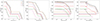 |
Fig. 1. Internal profiles of the TRAPPIST-1 planets computed with the BurnMan code. The panels show, from left to right, the density profile, the temperature profile, the viscosity profile, and the shear modulus profile. |
2.2.2. Love numbers
Love numbers were computed following the method of Tobie et al. (2005, 2019) with the code LPG-Tide, which uses the radial profile of the density, viscosity, shear modulus, and seismic velocities. We used an Andrade rheology (Andrade 1910), which defines the complex compliance  as (Castillo-Rogez et al. 2011; Efroimsky 2012)
with η the shear viscosity, ω the excitation frequency, β and α two empirical parameters, and Γ the Gamma function. Figure 2 shows the Love numbers’ frequency dependences associated with the TRAPPIST-1 profiles presented in Sect. 2.2.1. The top panel of Fig. 2 represents the frequency dependence of the imaginary part of the Love number, and thus the dissipation within each body (Tobie et al. 2005; Dumoulin et al. 2017; Bolmont et al. 2020a).
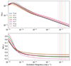 |
Fig. 2. Frequency dependence of the imaginary part (ℑ(k2); top panel) and real part (ℜ(k2); bottom panel) of the Love number of the TRAPPIST-1 planets assuming Earth-like compositions, computed from the profiles presented in Sect. 2.2.1 and Fig. 1. The vertical dotted lines correspond to each planet’s principal excitation frequency (i.e., the mean motion, n) if assumed to be perfectly synchronous. |
3. TRAPPIST-1 rotational states
We performed N-body simulations of the TRAPPIST-1 system. The rotational state was assumed to be synchronous at the beginning of the simulation. The orbital inclinations and obliquities of the planets were assumed to be zero, given the system’s high coplanar configuration and high tidal damping. The initial conditions were taken from Agol et al. (2021) and are listed in Table 1. The following section presents the evolution of the rotation state of each planet, their deviation from the synchronization state, and the variation in the position of the substellar points.
3.1. Non-synchronization
Figure 3 shows the variation of the rotation state, in terms of Ω/n (the spin rate over the mean motion), around the synchronization state for a period of 50 days. The simulation shows that none of the planets is perfectly synchronized; each oscillates around the synchronization state (i.e., Ω/n = 1) with different amplitudes and timescales. These variations are due to large mean motion variations caused by planet–planet interactions. As shown in Fig. 4 for planet e, the mean motion varies with such high amplitudes and on such short timescales that it prevents the synchronization of the spin.
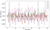 |
Fig. 3. Evolution of the rotation state of the TRAPPIST-1 planets in terms of Ω/n (the spin rate and the mean motion, respectively) around the synchronization state (Ω/n = 1). |
 |
Fig. 4. Spin rate and mean motion of planet e over 50 days. |
3.2. Substellar point drift
We computed the substellar position of each planet by subtracting the rotation angle (θ), computed from the integration of the spin rate, from the position angle (ν) of the star in the sky of the planet (the true anomaly), as ν − θ. Substellar points were computed to be zero after 50 years of simulation.
Variations of the spin states around the synchronization led to short- and long-term variations of substellar points. Figure 5 shows short-term variations, which correspond to short variations of the mean motion, as shown in Fig. 4. Amplitudes of low librations vary between 1 and 2 degrees depending on the planet, with a timescale that varies from about 1.5 days for planet b to 18 days for the planet h, which approximately corresponds to the orbital period of each planet. Figure 6 shows long-term drifts of the substellar point of each planet for a period of 250 years. The time needed for the substellar points to perform a complete rotation (i.e., the duration of the synodic day) varies between 55 years and −290 years, depending on the planet, and is summarized in Table 2. The estimations of planets T1-e, g, and h (in gray) should be taken with caution, as they appear to be strongly tidally locked and have not completed a single synodic rotation in 250 yr. A positive drift corresponds to a retrograde rotation with respect to its orbit, while a negative drift corresponds to a prograde rotation. We must highlight that the formalism used does not take the triaxiality of the planets into account. Therefore, considering the absence of the restoring force in the permanent deformation, these estimations correspond to the maximum theoretical drift due to the mean motion variations. Accounting for the triaxiality should lead to a stronger tidal torque (Van Hoolst et al. 2013) and, thus, reduce the drift rate. The triaxiality, which is expected to be particularly pronounced for this close-in planet due to strong permanent tidal forces, should further limit the drift. Interestingly, the two inner planets have the strongest drifts of the system despite their shorter distances to the star, and they are drifting in the opposite direction. We find that the drift is linked to the position of the planets in the resonance chain and leads to strong planet-planet interactions Planet b also shows numerical artifacts that make the computation of the substellar point challenging for a symplectic integrator. The combination of the very short orbital period and the shape of the Love number makes the dissipation in the low-frequency regime on the dissipation spectrum (see the top panel of Fig. 2).
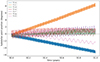 |
Fig. 5. Short-term librations of substellar points of the TRAPPIST-1 planets, in degrees, for a period of 1 year. Positive angles correspond to eastward drifts and negative angles to westward drifts. An eastward (respectively westward) rotation corresponds to a prograde (respectively retrograde) rotation of the planet with respect to its orbit. |
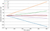 |
Fig. 6. Long-term variation of substellar points of the TRAPPIST-1 planets for a period of 250 years. Horizontal dotted lines represent multiples of 2π rotation. |
Estimation of the length of the day of the TRAPPIST-1 planets according to the rotation period of their substellar point.
4. Conclusion
This Letter presents recent developments made in the code Posidonius (Blanco-Cuaresma & Bolmont 2017; Bolmont et al. 2020a), i.e. the implementation of the Kaula formalism, that accounts for a realistic frequency dependence of the tidal response (Kaula 1964). We applied our work to the TRAPPIST-1 system and studied for the first time the variation of the spin of each planet around the synchronization state, accounting for the forcing of the tidal bulge and only assuming a realistic tidal model. We modeled the tidal response of each planet with the rheology of Andrade (1910) following the method of Bolmont et al. (2020a) with a multi-layered internal structure computed with the internal structure code BurnMan (Cottaar et al. 2014; Myhill et al. 2021).
We find that, despite the strong tidal interactions in the system, the spin of each planet is not perfectly synchronized (i.e., the spin rate of the planets is not strictly equal to their mean motion). Planet–planet interactions significantly perturb the mean motion of planets in compact configurations which prevents spin rates from remaining synchronous and causes the planets to oscillate around the synchronization state. As a consequence of these oscillations, planets experience variations of the position of their substellar point, leading to a slow and continuous drift. Continuous drifts lead the substellar points to perform complete rotations, which lead to day-night cycles, on retrograde rotation, with synodic day periods varying from 55 to 290 years depending on the planet.
We must highlight that the triaxiality of each planet is not taken into account in this study. It is still uncertain how the long-term shape of the planet evolves with respect to the spin-orbit evolution. On the one hand, if the spin and the orbit evolve on a timescale much shorter than the interior relaxation timescale, the planet would not have time to develop a permanent long-axis deformation in the star direction, and the planet should remain axisymmetric. On the other hand, if the spin orbit evolves on a much longer timescale than the relaxation timescale, a permanent long axis would develop and counteract any planet drift. Even under this condition, a drift is still possible, and the drift rate will be controlled by the rate at which the planet shape can readjust as the spin orbit changes. As we neglected the distorted shape of the planets and their long-term evolution, the estimations we obtain here should be considered as maximum synodic days from the spin oscillations around the synchronization state. Correia & Delisle (2019) evaluated the damping of the triaxiality due to mean motion variations but assumed a fixed permanent deformation (assuming that the triaxiality of the planet has two components, the permanent deformation due to the intrinsic mass repartition in the planet and the tidally induced deformation; see also Appendix D of Delisle et al. 2017).
Nonsynchronous spin states of TRAPPIST-1 planets have already been suggested, the first time by Makarov et al. (2018) to be spin-orbit resonances and/or pseudo-synchronization from the eccentricities of the system. However, our findings show not only eccentricities but the overall non-Keplerian shapes of the orbits due to planet–planet interactions. These interactions have been studied by Vinson et al. (2019), Shakespeare & Steffen (2023), and Chen et al. (2023), but their results differ from our findings on several points.
In particular, Vinson et al. (2019) and Shakespeare & Steffen (2023) identified several regimes of rotation coming from the pendulum effect caused by the triaxiality of planets. But firstly, they did not compute the spin rate in a full consistent way with their N-body simulation. Secondly, the tidal model used was the common CTL model (Hut 1981; Eggleton et al. 1998), which is not well suited for studying the rotation of rocky planets subjected to tides (Makarov & Efroimsky 2013).
Our study is the first to analyze the spin state of rocky planets while accounting for their internal structure. The drifts of substellar points depend on the competition between mean motion variation and tidal damping timescales, which are influenced by the strength of the tides and, thus, by the internal structure and the potential presence of a surface magma or water ocean. Future work will further investigate the trend of the substellar drifts and provide a detailed analysis of the impact of tidal models used and the rheological properties and internal structures of TRAPPIST-1 planets. In this study, we assumed TRAPPIST-1 planets have a metallic core and a silicate mantle, which is particularly relevant for the inner planets (b, c, and d). However, the low bulk density of the outer planets (e, f, and g) suggests they have significant volatile content and may also be compatible with the presence of water or ice (e.g., Unterborn et al. 2018; Boldog et al. 2024). Exploring a broader range of internal structures is beyond the scope of this study but will be crucial for understanding the physical and thermal processes of these exoplanets, as well as for the interpretation of observational data and assessing the potential habitability of these planets
Acknowledgments
AR and EB acknowledge the financial support of the SNSF (grant number: 200021_197176 and 200020_215760). The authors thank the referee, Michael Efroimsky, who provided good criticisms that help to improve our work. This work has been carried out within the framework of the NCCR PlanetS supported by the Swiss National Science Foundation under grants 51NF40_182901 and 51NF40_205606. The computations were performed at University of Geneva on the Baobab and Yggdrasil clusters. This research has made use of NASA’s Astrophysics Data System.
References
- Agol, E., Dorn, C., Grimm, S. L., et al. 2021, PSJ, 2, 1 [NASA ADS] [Google Scholar]
- Andrade, E. N. D. C. 1910, Proc. R. Soc. London Ser. A, 84, 1 [NASA ADS] [CrossRef] [Google Scholar]
- Andrade, E. N. D. C. 1914, Proc. R. Soc. London Ser. A, 90, 329 [NASA ADS] [CrossRef] [Google Scholar]
- Blanco-Cuaresma, S., & Bolmont, E. 2017, EWASS Special Session 4 (2017): Star-planet Interactions (EWASS-SS4-2017) [Google Scholar]
- Boldog, Á., Dobos, V., Kiss, L. L., van der Perk, M., & Barr, A. C. 2024, A&A, 681, A109 [NASA ADS] [CrossRef] [EDP Sciences] [Google Scholar]
- Bolmont, E., Raymond, S. N., Leconte, J., Hersant, F., & Correia, A. C. M. 2015, A&A, 583, A116 [NASA ADS] [CrossRef] [EDP Sciences] [Google Scholar]
- Bolmont, E., Breton, S. N., Tobie, G., et al. 2020a, A&A, 644, A165 [NASA ADS] [CrossRef] [EDP Sciences] [Google Scholar]
- Bolmont, E., Demory, B. O., Blanco-Cuaresma, S., et al. 2020b, A&A, 635, A117 [EDP Sciences] [Google Scholar]
- Boué, G., Correia, A., & Laskar, J. 2019, ApJ, 82, 91 [Google Scholar]
- Castillo-Rogez, J. C., Efroimsky, M., & Lainey, V. 2011, J. Geophys. Res. (Planets), 116, E09008 [CrossRef] [Google Scholar]
- Cayley, A. 1861, MmRAS, 29, 191 [NASA ADS] [Google Scholar]
- Chen, H., Li, G., Paradise, A., & Kopparapu, R. K. 2023, ApJ, 946, L32 [NASA ADS] [CrossRef] [Google Scholar]
- Correia, A. C. M., & Delisle, J.-B. 2019, A&A, 630, A102 [NASA ADS] [CrossRef] [EDP Sciences] [Google Scholar]
- Cottaar, S., Heister, T., Rose, I., & Unterborn, C. 2014, Geochem. Geophys. Geosyst., 15, 1164 [NASA ADS] [CrossRef] [Google Scholar]
- Delisle, J. B., Correia, A. C. M., Leleu, A., & Robutel, P. 2017, A&A, 605, A37 [NASA ADS] [CrossRef] [EDP Sciences] [Google Scholar]
- Dumoulin, C., Tobie, G., Verhoeven, O., Rosenblatt, P., & Rambaux, N. 2017, J. Geophys. Res. (Planets), 122, 1338 [NASA ADS] [CrossRef] [Google Scholar]
- Efroimsky, M. 2012, Celest. Mech. Dyn. Astron., 112, 283 [NASA ADS] [CrossRef] [Google Scholar]
- Efroimsky, M., & Makarov, V. V. 2013, ApJ, 764, 26 [NASA ADS] [CrossRef] [Google Scholar]
- Efroimsky, M., & Makarov, V. V. 2014, ApJ, 795, 6 [NASA ADS] [CrossRef] [Google Scholar]
- Eggleton, P. P., Kiseleva, L. G., & Hut, P. 1998, ApJ, 499, 853 [NASA ADS] [CrossRef] [Google Scholar]
- Gillon, M., Triaud, A. H. M. J., Demory, B.-O., et al. 2017, Nature, 542, 456 [NASA ADS] [CrossRef] [Google Scholar]
- Goldreich, P. 1966, AJ, 71, 1 [NASA ADS] [CrossRef] [Google Scholar]
- Goldreich, P., & Soter, S. 1966, Icarus, 5, 375 [Google Scholar]
- Gomes, G. O., Bolmont, E., & Blanco-Cuaresma, S. 2021, A&A, 651, A23 [NASA ADS] [CrossRef] [EDP Sciences] [Google Scholar]
- Greene, T. P., Bell, T. J., Ducrot, E., et al. 2023, Nature, 618, 39 [NASA ADS] [CrossRef] [Google Scholar]
- Henning, W. G., O’Connell, R. J., & Sasselov, D. D. 2009, ApJ, 707, 1000 [Google Scholar]
- Hirose, K., Wood, B., & Vočadlo, L. 2021, Nat. Rev. Earth& Environ., 2, 645 [NASA ADS] [CrossRef] [Google Scholar]
- Hut, P. 1981, A&A, 99, 126 [NASA ADS] [Google Scholar]
- Ih, J., Kempton, E. M. R., Whittaker, E. A., & Lessard, M. 2023, ApJ, 952, L4 [CrossRef] [Google Scholar]
- Kaula, W. M. 1961, Geophys. J., 5, 104 [NASA ADS] [CrossRef] [Google Scholar]
- Kaula, W. M. 1964, Rev. Geophys. Space Phys., 2, 661 [Google Scholar]
- Lincowski, A. P., Meadows, V. S., Zieba, S., et al. 2023, arXiv e-prints [arXiv:2308.05899] [Google Scholar]
- Makarov, V. V., & Efroimsky, M. 2013, ApJ, 764, 27 [Google Scholar]
- Makarov, V. V., Berghea, C. T., & Efroimsky, M. 2018, ApJ, 857, 142 [CrossRef] [Google Scholar]
- Myhill, R., Cottaar, S., Heister, T., Rose, I., & Unterborn, C. 2021, https://doi.org/10.5281/zenodo.5552756 [Google Scholar]
- Shakespeare, C. J., & Steffen, J. H. 2023, Bull. Am. Astron. Soc., 54, 203.04 [Google Scholar]
- Tisserand, F. 1889, Traité de mécanique céleste: Tome I, Perturbations des planètes d’après la méthode de la variation des constantes arbitraires (Gauthier-Villars) [Google Scholar]
- Tobie, G., Mocquet, A., & Sotin, C. 2005, Icarus, 177, 534 [Google Scholar]
- Tobie, G., Grasset, O., Dumoulin, C., & Mocquet, A. 2019, A&A, 630, A70 [NASA ADS] [CrossRef] [EDP Sciences] [Google Scholar]
- Unterborn, C. T., Desch, S. J., Hinkel, N. R., & Lorenzo, A. 2018, Nat. Astron., 2, 297 [NASA ADS] [CrossRef] [Google Scholar]
- Van Hoolst, T., Baland, R.-M., & Trinh, A. 2013, Icarus, 226, 299 [NASA ADS] [CrossRef] [Google Scholar]
- Vinson, A. M., Tamayo, D., & Hansen, B. M. S. 2019, MNRAS, 488, 5739 [NASA ADS] [CrossRef] [Google Scholar]
- Zieba, S., Kreidberg, L., Ducrot, E., et al. 2023, arXiv e-prints [arXiv:2306.10150] [Google Scholar]
Appendix A: Table of the inclination and eccentricity polynomials
The eccentricity polynomials Glpq(e) are elliptic expansions given by Eqs. 23 and 24 of Kaula (1961) and can be computed from the Hansen functions  (Cayley 1861; Tisserand 1889). They are presented in the Table A.1.
We considered eccentricities up to 0.3, which allowed us to study the eccentricity expansions up to order 7 (see the tables in Cayley 1861). As the tidal interactions are computed at the quadrupolar order l = 2, the index p is constrained between 0 and 2 and q between −7 and 7. The elements G22q(e) can be computed with the symmetry rule G2, 2, q(e)=G2, 0, −q(e).
Eccentricity polynomials, Glpq(e), from Cayley (1861), up to order 7 in eccentricity.
In practice, the order of the summation over q is taken as a function of the value of the eccentricity. The maximum order considered is listed in Table A.2.
Maximum order of the summation over q as a function of the eccentricity.
All Tables
Estimation of the length of the day of the TRAPPIST-1 planets according to the rotation period of their substellar point.
Eccentricity polynomials, Glpq(e), from Cayley (1861), up to order 7 in eccentricity.
All Figures
|
Fig. 1. Internal profiles of the TRAPPIST-1 planets computed with the BurnMan code. The panels show, from left to right, the density profile, the temperature profile, the viscosity profile, and the shear modulus profile. |
| In the text | |
|
Fig. 2. Frequency dependence of the imaginary part (ℑ(k2); top panel) and real part (ℜ(k2); bottom panel) of the Love number of the TRAPPIST-1 planets assuming Earth-like compositions, computed from the profiles presented in Sect. 2.2.1 and Fig. 1. The vertical dotted lines correspond to each planet’s principal excitation frequency (i.e., the mean motion, n) if assumed to be perfectly synchronous. |
| In the text | |
|
Fig. 3. Evolution of the rotation state of the TRAPPIST-1 planets in terms of Ω/n (the spin rate and the mean motion, respectively) around the synchronization state (Ω/n = 1). |
| In the text | |
|
Fig. 4. Spin rate and mean motion of planet e over 50 days. |
| In the text | |
|
Fig. 5. Short-term librations of substellar points of the TRAPPIST-1 planets, in degrees, for a period of 1 year. Positive angles correspond to eastward drifts and negative angles to westward drifts. An eastward (respectively westward) rotation corresponds to a prograde (respectively retrograde) rotation of the planet with respect to its orbit. |
| In the text | |
|
Fig. 6. Long-term variation of substellar points of the TRAPPIST-1 planets for a period of 250 years. Horizontal dotted lines represent multiples of 2π rotation. |
| In the text | |
Current usage metrics show cumulative count of Article Views (full-text article views including HTML views, PDF and ePub downloads, according to the available data) and Abstracts Views on Vision4Press platform.
Data correspond to usage on the plateform after 2015. The current usage metrics is available 48-96 hours after online publication and is updated daily on week days.
Initial download of the metrics may take a while.