| Issue |
A&A
Volume 644, December 2020
|
|
|---|---|---|
| Article Number | A26 | |
| Number of page(s) | 8 | |
| Section | Stellar atmospheres | |
| DOI | https://doi.org/10.1051/0004-6361/202038175 | |
| Published online | 26 November 2020 | |
Keeping up with the cool stars: one TESS year in the life of AB Doradus
Hamburger Sternwarte Universität Hamburg,
Gojenbergsweg 112,
21029
Hamburg,
Germany
e-mail: This email address is being protected from spambots. You need JavaScript enabled to view it.
Received:
15
April
2020
Accepted:
20
October
2020
Abstract
The long-term, high precision photometry delivered by the Transiting Exoplanet Survey Satellite (TESS) enables us to gain new insight into known and hitherto well-studied stars. In this paper, we present the result of our TESS study of the photospheric activity of the rapid rotator AB Doradus. Due to its favorable position near the southern ecliptic pole, the TESS satellite recorded almost 600 rotations of AB Doradus with high cadence, allowing us to study starspots and flares on this ultra-active star. The observed peak-to-peak variation of the rotational modulations reaches almost 11%, and we find that the starspots on AB Doradus show highly preferred longitudinal positions. Using spot modeling, we measured the positions of the active regions on AB Doradus and we find that preferred spot configurations should include large regions extending from low to high stellar latitudes. We interpret the apparent movement of spots as the result of both differential rotation and spot evolution and argue that the typical spot lifetimes should range between 10 and 20 days. We further find a connection between the flare occurrence on AB Doradus and the visibility of the active regions on its surface, and we finally recalculated the star’s rotation period using different methods and we compared it with previous determinations.
Key words: stars: activity / stars: rotation / stars: flare / starspots / techniques: photometric / methods: data analysis
© ESO 2020
1 Introduction
While the study of stellar activity has been the focus of many observational and theoretical research efforts over the last decades, we are still not in a position to fully understand and cope with all of its effects on time-series observations. The latter has been revolutionized during the last decade as a consequence of the availability of high-precision, long term, and essentially uninterrupted space-based photometry, as delivered by the CoRoT (Auvergne et al. 2009), Kepler (Borucki et al. 2010), and Transiting Exoplanet Survey Satellite (TESS) missions (Ricker et al. 2015), which provided and still provides data of unsurpassed quality that is unachievable from the ground.
In such photometric observations, one typically sees light curve modulations caused by the periodic appearance and disappearance of active regions in the stars’ photosphere, that is to say star spots. As we know from the Sun, sunspots rotate with the Sun and produce depressions in the observed solar flux (see an overview by Fröhlich 2012). Therefore, one expects stellar observations to provide similar information on star spots, and many studies are dedicated to understanding how and where star spots form, how long they live, and how those characteristics depend on the age and type of the underlying star.
A great new research opportunity has opened up with TESS (Ricker et al. 2015). With its anticipated observation strategy, TESS will cover >80% of the sky and therefore, unlike the cases of CoRoT and Kepler, also deliver high-precision space-based photometry for brighter stars that are already well known and intensely studied at other wavelengths. One such star is AB Doradus, which is a bright, nearby, rapidly rotating, and very active star. It is fortuitously located at rather high ecliptic latitudes and was almost continuously observed by TESS in its first year of operation. In this paper, we present almost one year (298 days) of TESS observations of AB Dor and carry out an in-depth analysis of its photometric activity features, as observed by TESS.
2 Observations
2.1 The TESS mission
The TESS mission is dedicated to the discovery of transiting exoplanets around bright stars (see Ricker et al. 2015) via photometry. To this end, TESS was designed to cover a very large sky area (24° × 96°) utilizing four wide-field cameras. The initial two-year observation strategy of TESS includes 26 sectors, 13 of which are in the southern ecliptic hemisphere, the other 13 are in the northern ecliptic hemisphere, and each is continuously observed for 27 days. As a result, those parts of the sky that are closer to the ecliptic poles are observed for longer periods than 27 days with a maximum observation time of one year around the ecliptic poles. TESS’s primary scientific goal is to survey the brightest 200 000 stars for transiting exoplanets. The actual light curves of those bright stars are produced by the Science Processing Operation Center (SPOC) pipeline (see, Jenkins et al. 2016)and are publicly accessible and available for download from the Mikulski Archive for Space Telescopes (MAST)1.
2.2 AB Doradus
The star we focus on in this study is AB Dor A. It is the brightest member of a system with four stars in total (Guirado et al. 2011). However, due to the brightness contrast of AB Dor A and its companions, we ignore those in the following and thus refer to AB Dor A as AB Dor for simplicity. In Table 1 we show some basic information about AB Dor.
As a foreground star of the Large Magellanic Cloud, AB Dor was first recognized as an interesting (flaring) X-ray stellar source by Pakull (1981), who measured its rapid rotation (Prot = 0.514 d) and interpreted AB Dor as a new RS CVn system. Innis et al. (1988a) presented high-resolution spectroscopy of AB Dor, showing it to be a single star, and the photometry of AB Dor, covering the period from 1978–1987. It was suggested that “AB Dor had two large, long-lived starspots during this period” (Innis et al. 1988b).
Given its short rotation period of a little over half a day, AB Dor can be Doppler imaged much more easily than longer period stars. Using observations taken in February 1989, Kuerster et al. (1994) presented the spatial distribution of starspots using Doppler images, which also show similarities with the spot distribution discussed by Innis et al. (1988b). Moreover, Kuerster et al. (1994) showed a consistency of their pseudo-simultaneous photometry with the derived Doppler images. Furthermore, their Doppler images suggest an inclination angle of about 60° between the stellar rotation axis and the line of sight. Donati & Collier Cameron (1997) derived the differential rotation of AB Dor and showed that it is rotating, almost as a rigid body. Further studies of the differential rotation of AB Dor based on Doppler imaging have been presented by Collier Cameron & Donati (2002), Donati et al. (2003), and Jeffers et al. (2007). The latter authors present a sequence of Doppler images of AB Dor, which were constructed from data taken in December 1988, January and December 1992, and November 1993 and 1994, with special emphasis on the differential rotation of AB Dor.
Extensive X-ray studies of AB Dor have been presented, for example, by Kuerster et al. (1997), who discuss the ROSAT data on AB Dor, and by Lalitha et al. (2013), who present simultaneous XMM-Newton and VLT observations of AB Dor which, in particular, cover a very large flare. This flare was also studied by Schmitt et al. (2019), who show the superflare nature of such flares observed by TESS during the first two months of data taking. Thus, in summary, according to our current understanding, AB Dor is rather nearby (d = 15.3 pc), ultra-active, and a pre-main-sequence object with a radius of 0.96 ± 0.06 R⊙ (see Guirado et al. 2011), which shows strong signatures of magnetic activity at all wavelengths.
Basic information on AB Dor.
3 Results
3.1 Light curve
The apparent brightness of AB Dor (mV = 7 mag) makes it one of the brightest stars observable by TESS, which, in combination with the scintillation-free environment of space, results in a light curve with a very high signal-to-noise ratio. Due to the long TESS observation time of AB Dor and its short rotation period, the traditional representation of the light curve as a time series does not allow us to explore the variations in the time series in detail. Thus we chose to use a time-brightness diagram to show the total light curve of AB Dor in a more compact and readable fashion.
For the construction of the time-brightness plot, we split the light curve in chunks of length equal to the period derived by Schmitt et al. (2019), that is, 0.514275 days. Assuming that this signal’s period is indeed the star’s rotation period, each of these chunks then represents one rotation of AB Dor. Each chunk is plotted in time order from bottom to top, which provides a better impression of the light curve’s temporal evolution. The bright parts of the plot show parts of the light curve with high stellar flux and, conversely, the darker parts of the plot are those parts of the light curve where the stellar flux is reduced.
In Fig. 1, we show the time-brightness diagram constructed using the TESS data set of AB Dor. The TESS light curve shows large peak-to-peak variations, which vary between ~6 and ~11%. We interpret those modulations as the result of star spots, which become visible as the star rotates; thus, we assume that the period of these variations is indeed the stellar rotation period. This signal is clearly periodic, and although it almost repeats itself perfectly from one period to the next, there are evident long-term variations that alter the apparent shape of the light curve with time. We also note that Fig. 1 shows only the contrast between the different areas of the stellar surface, that is, the bright areas of the plot are not necessarily free of star spots.
In addition to the rotation modulations, there are events with a rapid increase in the stellar flux followed by a more or less exponential decay, which we interpret as stellar flares. Schmitt et al. (2019) performed an in-detail analysis of those events for the first two sectors of the TESS data on AB Dor.
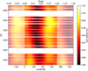 |
Fig. 1 Total TESS time series of AB Dor phased assuming a rotation period of Prot = 0.514275 days; see text for details. |
3.2 Activity modulations: period and amplitude
One of the most remarkable properties of AB Dor is its extremely rapid rotation. Consequently, it is not surprising that its period was measured several times by different authors; Table 2 provides some of those results and their references. Given the temporal evolution of the light curve and the divergence between the different measurements through the years, we did not attempt to measure the rotation period of the star using the total light curve. Instead, we split the light curve into different parts, assuming that in each part, the star has completed five rotations, and we used the generalized Lomb-Scargle periodogram (GLS; see Zechmeister & Kürster 2009) to measure the period of the activity modulations in each one of those parts. The results of our measurements are shown in the upper panel of Fig. 2. The modulation period appears to be relatively stable during the observations with an average of ~0.514843 days, except for the first ~50 days; we estimate the typical uncertainty of those period measurements to be on the order of one minute.
To connect this result with the phenomenology of the light curve and, given that the contrast between the dark and bright areas in Fig. 1 (i.e., the peak-to-peak variation of the light curve) reaches its maximum value between TJD ≃ 1500 days and TJD ≃ 1580 days2, we also measured the average peak-to-peak variation of the same parts of the light curve, which we show in the lower panel of Fig. 2. We estimate the typical error for those measurements to be on the order of 10−4.
At first sight, the GLS results and the peak-to-peak variation of the light curve, as presented in Fig. 2, show no direct correlation between them or between the GLS results and the phenomenology of the light curve (i.e., the relative “motion” of the dark areas in Fig. 1). Given the possible inadequacy of the GLS periodogram to describe a light curve that can hardly be described as sinusoidal due to its continually evolution, we attempted to measure the period of the modulationsusing yet another method, that is, to measure the time distance between consecutive minima and maxima, to which we refer to as min-max in the following. Again, we estimate the typical uncertainty of those measurements to be on the order of one minute.
In Fig. 3 we show the results of our min-max measurements. The upper panel is explanatory and shows what we mean by the terms minima (orange), maxima (green), and their difference (purple), using a part of the actual TESS light curve of AB Dor. We note that the precision of the measurements is so large that the error bars are smaller than the dots in this plot. As shown in Fig. 3, the values of δmin = 0.51396 days and δmax = 0.51488 days are stable in time but not equal (see Table 2), although the difference of their average values appears to be insignificant. We also measured the min-max difference (depicted with purple in Fig. 3) to test how the time difference between minima and maxima varies during the observations of AB Dor. The results, shown in the lower panel of Fig. 3, suggest that the measured differences between theconsecutive minima and maxima appear to be time-dependent, quantify the phenomenology of the light curve shownin Fig. 1, and agree with the peak-to-peak variations shown in Fig. 2.
AB Dor rotation periods measured by other authors using photometry and this work.
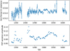 |
Fig. 2 Top panel: variation of the GLS periodogram of the light curve of AB Dor, split into parts containingfive rotations each. We note that the reduced error sizes in the time range between 1500 ≲ TJD ≲ 1550 are related to the shape of the light curve during that time (which is closer to sinusoidal than the rest of the light curve) and the GLS periodogram’s ability to measure the periods of sinusoidal-like signals more accurately. Bottom panel: mean peak-to-peak variation amplitude assuming sets of five rotations (the y-axis is in normalized flux units). |
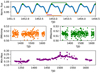 |
Fig. 3 Min-max measurements. One can see a definition of the terms minima (orange), their difference δmin (orange line), maxima (green), their difference δmax (green line), and the difference min-max (purple line); their distributions (middle panels); and the evolution of their difference (bottom panel). |
3.3 Spot modeling
The known inclination of AB Dor allowed us to use a spot model to derive the location of the spots on the stellar surface. This type of spot modeling has been applied to photometric light curves for a long time and the difficulties encountered are succinctly described, for example, by Harmon & Crews (2000). In principal, one is trying to reconstruct a 2D-surface from 1D data (i.e., a light curve),and such problems are known as “ill-posed” in the mathematical literature. To overcome these difficulties, one either has to choose some kind of regularization, that is to say surfaces as have to be as “smooth” as possible, for example, or one has to limit the number of free parameters, that is, the number of spots on the surface and hence the number of free parameters. It is a difficult problem to decide how many free parameters one needs, in practice, to describe a given light curve. We estimate the number to be in the range of eight to ten from numerical experiments. At any rate, it must be clear that the inherentmathematical difficulties of any light curve inversion does not allow for the construction of unique models.
To measure the positions of the star spots on AB Dor, we, therefore, used a 3+2 spot model similar to the one described and used by Ioannidis & Schmitt (2016) with the difference that the spots are not locked onto the stellar equator, but rather they may take latitude values as large as 60°. The numberof spots in our spot model remains constant for modeling each phase of the light curve. Although our model assumes nonoverlapping circular spots, we think of those areas more like large active regions consisting of many unresolved, little spots, rather than a large uniform spot. Furthermore, our spot models assumes a spot temperature of tsp = 0, due to the correlation of tsp with the spot radius. An impression of a typical modeling result is given in Fig. 4, which shows the modeled spotted surface of AB Dor at two epochs close to the mean and average high peak-to-peak variation in an Aitoff projection. The more detailed results of our spot model are shown in Fig. 5, which provides the temporal evolution of longitudes of the derived spot positions. As we show in Fig. 5, our model suggests the existence of a spot, separated by approximately 120° by a pair of other spots early in the TESS observations. The angular separation of the spots becomes smaller as time goes by, reaching its smallest value (i.e., ~100°) between TJD ≃ 1500 days and TJD ≃ 1550 days. Just before the end of the TESS observations, the spots appear to move “back” to a point close to their original positions.
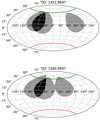 |
Fig. 4 Aitoff projections of the spot configuration on AB Dor at TJD = 1452.9647 (upper plot) and TJD = 1540.0947 (lower plot). |
3.4 Flares
As is shown by Schmitt et al. (2019), the TESS light curve of AB Dor shows many “big” flares. Although the goal of this study is not to focus specifically on the flares, we used the big flares (as defined by Schmitt et al. 2019) to measure their temporal distribution. The detection and categorization of the flares was achieved manually. Specifically, we visually inspected the TESS light curve of AB Dor and identified the flares with peak luminosities larger than 1 × 1031 erg s−1 (i.e., ~0.5% in the AB Dor light curve); as flare occurrence times, we used the time just when the rising phase of the flare began.
Following this procedure, we manually identified 87 big flares in the TESS light curve of AB Dor, that is to say a little more than two of those flares per week. In Figs. 6 and 7, we show the distribution of these big flares as a function of time as well as rotation phase (assuming a rotation period of Prot = 0.514275 days), respectively.The red lines denote the observation coverage rate for both figures, where “0” denotes no observations. Although we do not detect significant variations or trends with time, it becomes clear from Fig. 7 that there is a preferential behavior of the flare occurrence related to the rotation period of the star: there is ~55% lower majorflare occurrence between phase 0.6 and 0.8 with a significantly more than 2σ (assuming that the flare occurrence follows a Poisson distribution). In comparison to Fig. 1, we note that this is exactly that part of the light curve when the star is less spotted, which is consistent with the view that there are fewer flares when there are fewer spots.
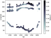 |
Fig. 5 Spot modeling result for the light curve of AB Dor. The measured sizes of the spots (in R⋆ units) appear in grayscale. |
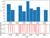 |
Fig. 6 Distribution of “big” flares of AB Dor during the TESS observation time. |
4 Discussion and conclusions
4.1 Rotation period
As apparent from Table 2, the rotation period of AB Dor is in the range between Prot = 0.51396 days and Prot = 0.51488 days. However, we can obtain a more precise measurement if we assume that the bright parts in the light curves of AB Dor, that is, the phase range 0.25 < ϕ < 0.5, is not changing its position on the star. Under this assumption, we can calculate AB Dor’s rotation period by combining the photometric data from Kuerster et al. (1994) and TESS. Kuerster et al. (1994) listed their photometry times, from which we can derive the time of maximum light during their observations as T0 = 2 447 579.5307. In the TESS light curve, we find one of its maxima at the time T1 = 2 458 473.0. By assuming a certain number of rotations, we can then reproduce the different rotation periods derived in the literature; we show in the third column of Table 2 these values, which range from 21 160 and 21 195. The rotation period derived by Schmitt et al. (2019) was also derived from the period between maximum light epochs, and thus, under our assumption that maximum light occurs at the same rotation phase, some 21 181 AB Dor “days” would have elapsed, which leads to a period of Prot = 0.51430 days.
4.2 Spot positions
During the whole TESS observation process of AB Dor, there was not a single moment when the star was spotless, that is, at least in the zone below 60° latitude. AB Dor does not seem to be special in that manner, and there are many examples of other stars with similar long-term behavior, yet, remarkably, we seem to have somehow observed the same set of active regions. The similarity ofour results, as seen in Fig. 4, with those shown in Figs. 12–15 by Kuerster et al. (1994) suggest thatthe active regions formation on AB Dor’s surface has changed only a little or not at all for the last ~30 yr, which is in agreement with our measurements from Sect. 4.1.
The results of our spot model analysis suggest that the spots on AB Dor appear at relatively low latitudes in the range of 20 ° < ϕ < 30°. The low latitudes result from the fact that the model needs to account for the observed substantial peak-to-peak variations. This is not in contradiction with the assumption of polar spots, which would drop the star’s total observed flux and only contribute to the rotational modulation on a lower scale. Although we used zero spot temperatures in our model, the calculated active region sizes are still enormous for solar standards. Although we cannot accept or reject those results, such spot formation scenarios appear nonphysical, suggesting that there may be alternative explanations for the measured peak-to-peak variation.
AB Dor is one of the best candidates to apply a spot model, and we can be confident that the longitude results, shown in Fig. 5, reflect the reality. However, if the evolution of the active regions was to follow what Fig. 5 suggests, the active regions of AB Dor should alter their differential rotation patterns (i.e., the rotation period of the active regions would have to change dramatically at TJD ~ 1525 days). As aresult, we think that the “change in course” observed at TJD ~ 1525 is connectedwith the appearance, evolution, and disappearance of smaller spot groups (parts of the larger active regions) and not a consequence of differential rotation.
During the phases with visible spot features, we see 40% more flares. This implies that (1) the flares occurrence is directly connected to the spot occurrence and (2) 60% of the flares should occur in areas with constant spot visibility, that is, the polar cap.
4.3 Spot lifetimes
Although the formation of the active regions in the photosphere of AB Dor seems to be restricted in longitude, the temporal evolution of the light curve does suggest that we are not looking at the same active regions all the time. Rather, the modulations of AB Dor are created by starspots, which are born, evolve, and eventually dissolve around the same general active longitude (see Fig. 1 between phase ~0.25 and ~0.6).
To this end, we inspected the GLS periodogram of the TESS AB Dor light curve, which is also in the period range above five days and which identified formally significant peaks in the period range between 11 and 30 days, with the most prominent peaks being located around 13 and 26 days. However, it is rather difficult to assess the true nature of those signals, given the observation strategy of TESS, that is, repointing the telescope every 27 days, a procedure which could introduce spurious periodicities in the GLS periodogram.
To better understand the nature of these additional signals in the GLS periodogram of AB Dor, we therefore followed a different approach and investigated the correlation structure of the TESS AB Dor light curve. Assuming a rotation period of Prot = 0.51488 days, we could phase the observed light curve of AB Dor and consider the light curve as a function of rotation or time. We then specifically cross-correlated the phased light curve of TESS’ first rotation of AB Dor with each phased light curve derived from the subsequently observed TESS rotations and we show the results of this procedure in Fig. 8, that is, we plotted the computed cross-correlation coefficient of the nth rotation (denoted by time in TJD) with respect to the first rotation. The points scattering around a correlation coefficient of zero are mainly caused by flares and other systematic errors in the light curve, yet the bulk of the data points (i.e., the correlation coefficients of the phased light curves) shown in Fig. 8 follow a clear pattern of increasing decorrelation until TJD 1500 (i.e., after ~350 rotations), from which point the cross-correlation starts increasing again.
The choice of the first observed rotation as a reference is, of course, arbitrary, and in fact, we can choose any rotation as a reference. More generally, we can compute a quadratic matrix Ci,j, which contains, as its elements, the cross-correlation coefficients computed between any of the observed rotations i = t0,..., tN, where ti denotes the central time of the ith rotation, and the light curve of the jth rotation as a reference; thus, by construction, Ci,i = 1, for i = 1, N, where N denotes the total number of rotations. To provide an example, the correlation coefficients shown in Fig. 8 refer to C1,j. Next, we investigated the process of decorrelation by determining the autocorrelation of the computed cross-correlation functions. Thus for the cross-correlation Ci,j (with the index i denoting time and the index j denoting the chosen reference rotation), we computed correlation coefficients Ak,j, with the index k denoting the chosen lag (in terms of rotations) and the index j again denoting the chosen reference rotation; hence by construction we have A0,j = 1. In Fig. 9 we show a few examples of such autocorrelation functions, namely those using rotation 1 as a reference (blue), rotation 300 (orange), and rotation 580 (green). In all of these functions, a “wiggly” structure with a period of about 26 rotations (i.e., around ~ 13 days) appears. In Fig. 10, we show – as a time-lag diagram – the full array of autocorrelations, with the x-axis displaying the lag and the y-axis showing the chosen reference rotation. In all functions, Ak,j, which is a sequence of vertical patterns, appears, which reflects the “wiggly” structure in Fig. 9. To obtain results independent of the reference rotation, we “collapsed” the matrix Ak,j along the y-axis, that is, computing the mean autocorrelation function 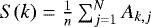 to finally arrive at Fig. 11, which again shows periodic modulations. It is, of course, suggestive of interpreting these modulations as signatures of spot lifetimes, and we note that at a period of 13 days, a peak in the GLS periodogram is found.
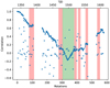 |
Fig. 8 Cross-correlation between the different rotations of AB Dor TESS light curve, using the first observed rotation in the same data as a reference (see text for details). |
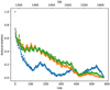 |
Fig. 9 Rows 0, 300 and 600 of the autocorrelation functions Ak,j from the AB Dor light-curve; see text for details. |
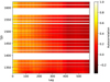 |
Fig. 10 Time-lag diagram of autocorrelation functions Ak,j. It is importantto note the decrease in correlation (see text for details). |
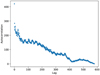 |
Fig. 11 Mean autocorrelation as function of lag for the light curve of AB Dor; see text for details. |
4.4 Spot simulations
To better understand the statistical properties of our TESS AB Dor light curve, we also simulated the photometric light curve of a star with the physical characteristics of AB Dor, that is, with active longitudes as they appear in Fig. 1, with constant spot coverage (see Sect. 4.2), and with similar temporal evolution as shown in Fig. 8. We note that the goal of this exercise is not to recreate the exact spot configuration on AB Dor, but rather to investigate whether (a) there is any spot configuration which would produce the pattern apparent in Fig. 11 without assuming an unrealistic light curve and (b) how the same pattern is related to the spot lifetimes, while at the same time keeping our model as simple as possible.
Via trial and error, we found that the simplest spot configuration to mimic a light curve satisfying our criteria requires a combination of five spots, that is, two spots at rather high latitudes (with Rsp ∕R⋆ = 0.05 and 70° latitudes) – with their larger parts in the continuously visible area of the star – and a set of three spots at lower latitudes (with 0.05 ≤ Rsp ∕ R⋆ ≤ 0.1), grouped in an area with similar longitudes and latitude values around 20°. In this fashion, we obtain a light curve without any flat parts, that is, at least one spot is always present on the visible hemisphere – a configuration which is in agreement with previous Doppler imaging studies on AB Dor (see, Donati & Collier Cameron 1997 and Jeffers et al. 2007). Next, we assumed solar-like-differential rotation following Donati & Collier Cameron (1997) to create the needed temporal evolution of the light curve and set the rotation periods for the high and low latitude spots equal to the maximum and minimum values listed in Table 2, respectively. To create lifetime effects, we assumed that the low latitude spots have similar but not exactly equal lifetimes (the mean value of which we set to 6, 12, and 24 days) in different simulations, while the high latitude spots remain constant. The difference in the lifetimes of the spots in a given spot group was set to 0.3 days (e.g., 11.7, 12, and 12.3 days). Since the appearance and disappearance of spots – based on our knowledge from solar spots – is not instantaneous, we describe these effects with an ad hoc “smoothing function” and assume that the appearance and disappearance are described by half of a cosine wave via the function  = Rspot × (cos(T + π) + 1)∕2 during growth and
  = Rspot × (cos(T) + 1)∕2 during the decay, where the dimensionless time T is the ratio between actual time t and the spot lifetime tsp via T = t (2π tsp)−1. In our simulations, the growth or the decay of the spots was arbitrarily set to last 2.5 days. After the disappearance of a spot, a new spot with the same characteristics replaced it immediately in the same position. To avoid sampling biases, we kept the total number of days in our simulated light curve equal to the observation time. Additionally, for simplicity, the maximum size of all spots remained the same during the total time of the simulated light curve, and it was set so the peak-to-peak of the variations matched the real AB Dor light curve. In this fashion, we generated synthetic light curves choosing spot lifetimes of 6, 12, and 24 days, which were then subject to the same analysis as the real AB Dor TESS light curves.
The time-lag diagram of our simulated light curves analogous to Fig. 10 is shown in Fig. 12. Although there is great similarity between our simulations and the actual data from AB Dor, our case, that is to say that the peaks in the Ai,j are the result of spot lifetimes, becomes more clear when we compare the Ak,j from simulated light curves with various spot lifetimes. In Fig. 13 we show the collapsed Ak,j values for spots with lifetimes of 6, 12, and 24 days.
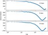 |
Fig. 13 Top panel: same as Fig. 11, but from our simulated light curve and assumed spot lifetime of 12 days. Middle and bottom panels: collapsed Aij from our simulated light curves for spots with assumed lifetimes of 6 and 24 days, respectively. |
4.5 Bright spots
As discussed in Sect. 4.2, the peak-to-peak variations in the AB Dor light curve suggest the size of the active regions to be very large, that is, the average spot size from our modeling is Rspot /R⋆ ≃ 0.18. On topof that, the temperature contrast between those regions and the stellar photosphere should be almost maximum (i.e., for our models, we assume Tspot/T⋆ = 0). Although we are not in a position to confirm or disprove of this hypothesis, in this section, we explore an alternative hypothesis, that is, the existence of bright regions in combination with “traditional” cool active regions. As we know from the Sun, during thoseperiods of the 11-yr cycle when it is more active and has more spots, it is also brighter in total solar irradiance due to the contribution of plage regions. Following a similar line of thought, we assume ad hoc that a similar process occurs in AB Dor, and, by using our spot model algorithm, we attempted to reproduce the observed modulations in the TESS light curves of AB Dor with both bright and dark spots as well as with bright spots alone. Although it is possible to replicate the modulations following both assumptions, the problem of the large active regions with high contrast remains. Specifically, it was not possible to recreate the activity modulations unless we used large (Rspot/R⋆ ≃ 0.1), cool (Tspot/T⋆ ≃ 0.3), and bright (Tspot/T⋆ ≃ 1.7). As a result, we conclude that assuming the presence of bright, active regions does not lead to less extreme values for the spot sizes and temperatures.
4.6 Differential rotation
As discussed in Sect. 2.2, ever since the “discovery” of AB Dor, its differential rotation of AB Dor has been the subject of quite a few studies. From their Doppler images, Donati & Collier Cameron (1997) derived a rotation “law” for AB Dor of the form Ω(l) = 12.2434 − 0.0564sin2(l) (rad day−1), where l denotes the stellar latitude, implying that the polar regions rotate more slowly than equatorial ones. Evaluating Ω(l) at a latitude of 30° yields a period of 0.513781 days, which is shorter than any of the periods derived from photometry (cf., Table 2). Similarly, analyzing Doppler images of AB Dor between 1988 and 1994, Jeffers et al. (2007) reported spectroscopic periods of 0.5142 d, 0.5139 d, and 0.5141 d for features at “effective” latitudes of 55.61°, 54.45°, and 56.78°, which translate into equatorial rotation periods of 0.5134 d, 0.5129 d, and 0.5132 d, respectively. Using photometry taken over 20 yr and the Occamian spot inversion techniques, Järvinen et al. (2005) estimated spot periods in the range of 0.51470 and 0.51487 d, which from their spot inversion models translates into simultaneously existing spot groups in high (>50°) and low (<30°) latitudes. Thus, in comparison, our photometric TESS results agree with the results of Järvinen et al. (2005).
5 Summary
In this paper, we present the results of one year of almost continuous high precision photometry of AB Dor with TESS, with a focus on the photospheric activity of the star. We measured the rotation period of the star using a variety of methods. Although our measurements of the rotation period of AB Dor differ between themselves as well as with past measurements (see Table 2), the difference is minimal (≲ 1 min). We find that the rotation period which fits the data best is Prot = 0.514275 days (Schmitt et al. 2019).
The rotation period of the star is stable during the TESS observation time. However, there appears to be some “movement” of spots, which manifests itself as differences in the distances between the minima and maxima of the activity modulations and is also visible in our spot model results. We interpret this movement to be due to spot evolution and differential rotation; the spots are not formed uniformly over the stellar surface and live only in highly preferred longitudinal regions. There is even evidence that the locations and the configuration of these active regions is similar to the ground-based observations presented by Kuerster et al. (1994) more than 40 yr ago. This of course does not mean that the spots on AB Dor live that long. In contrast, weargue through a detailed study of the light curve’s correlation structure that typical spot lifetimes range from between 10 and 20 days. In this data set, we do not see evidence of flip flop as reported by Järvinen et al. (2005).
Furthermore, AB Dor produces frequent flares; we note that we are likely to see only half the produced flares. When we see the hemisphere of the stars with low spottedness, there is a ~60% lower occurrence rate of big flares as compared to the case when the other hemisphere of the star is visible, confirming the straightforward picture that at least the big flares tend to occur in more heavily spotted areas. The fact that the flare occurrence rate does not drop to zero during the times that we “see” the unspotted part of the star may suggest that those flares are being produced in the ever-seen active regions close to the poles. This behavior is, of course, un-solar-like. While it usually is not possible to locate the flaring region on an unresolved stellar surface, the giant flare on Algol observed and described by Schmitt & Favata (1999) did occur in the polar region and might present a precedent for AB Dor.
Acknowledgements
This paper includes data collected by the TESS mission, which are publicly available from the Mikulski Archive for Space Telescopes (MAST). P.I. acknowledges funding through the DFG grant SCHM 1032/65-1. Furthermore, we would like to thank the anonymous referee for their comments, which helped improve our paper.
References
- Auvergne, M., Bodin, P., Boisnard, L., et al. 2009, A&A, 506, 411 [NASA ADS] [CrossRef] [EDP Sciences] [Google Scholar]
- Borucki, W. J., Koch, D., Basri, G., et al. 2010, Science, 327, 977 [NASA ADS] [CrossRef] [PubMed] [Google Scholar]
- Collier Cameron, A., & Donati, J. F. 2002, MNRAS, 329, L23 [NASA ADS] [CrossRef] [Google Scholar]
- Donati, J. F., & Collier Cameron, A. 1997, MNRAS, 291, 1 [NASA ADS] [CrossRef] [Google Scholar]
- Donati, J. F., Collier Cameron, A., Semel, M., et al. 2003, MNRAS, 345, 1145 [NASA ADS] [CrossRef] [Google Scholar]
- Fröhlich, C. 2012, Surv. Geophys., 33, 453 [NASA ADS] [CrossRef] [Google Scholar]
- Guirado, J. C., Marcaide, J. M., Martí-Vidal, I., et al. 2011, A&A, 533, A106 [NASA ADS] [CrossRef] [EDP Sciences] [Google Scholar]
- Harmon, R. O., & Crews, L. J. 2000, AJ, 120, 3274 [CrossRef] [Google Scholar]
- Innis, J. L., Thompson, K., Coates, D. W., & Evans, T. L. 1988a, MNRAS, 235, 1411 [NASA ADS] [CrossRef] [Google Scholar]
- Innis, J. L., Coates, D. W., & Thompson, K. 1988b, MNRAS, 233, 887 [NASA ADS] [Google Scholar]
- Ioannidis, P., & Schmitt, J. H. M. M. 2016, A&A, 594, A41 [NASA ADS] [CrossRef] [EDP Sciences] [Google Scholar]
- Järvinen, S. P., Berdyugina, S. V., Tuominen, I., Cutispoto, G., & Bos, M. 2005, A&A, 432, 657 [NASA ADS] [CrossRef] [EDP Sciences] [Google Scholar]
- Jeffers, S. V., Donati, J. F., & Collier Cameron, A. 2007, MNRAS, 375, 567 [NASA ADS] [CrossRef] [Google Scholar]
- Jenkins, J. M., Twicken, J. D., McCauliff, S., et al. 2016, SPIE Conf. Ser., 9913, 99133E [Google Scholar]
- Kuerster, M., Schmitt, J. H. M. M., & Cutispoto, G. 1994, A&A, 289, 899 [Google Scholar]
- Kuerster, M., Schmitt, J. H. M. M., Cutispoto, G., & Dennerl, K. 1997, A&A, 320, 831 [Google Scholar]
- Lalitha, S., Fuhrmeister, B., Wolter, U., et al. 2013, A&A, 560, A69 [NASA ADS] [CrossRef] [EDP Sciences] [Google Scholar]
- Pakull, M. W. 1981, A&A, 104, 33 [NASA ADS] [Google Scholar]
- Ricker, G. R., Winn, J. N., Vanderspek, R., et al. 2015, J. Astron. Telesc. Instrum. Syst., 1, 014003 [Google Scholar]
- Schmitt, J. H. M. M., & Favata, F. 1999, Nature, 401, 44 [NASA ADS] [CrossRef] [Google Scholar]
- Schmitt, J. H. M. M., Ioannidis, P., Robrade, J., Czesla, S., & Schneider, P. C. 2019, A&A, 628, A79 [CrossRef] [EDP Sciences] [Google Scholar]
- Zechmeister, M., & Kürster, M. 2009, A&A, 496, 577 [NASA ADS] [CrossRef] [EDP Sciences] [Google Scholar]
TJD is the TESS JD time, which is defined as the difference between the barycentric dynamical time minus the number 2 457 000.
All Tables
AB Dor rotation periods measured by other authors using photometry and this work.
All Figures
|
Fig. 1 Total TESS time series of AB Dor phased assuming a rotation period of Prot = 0.514275 days; see text for details. |
| In the text | |
|
Fig. 2 Top panel: variation of the GLS periodogram of the light curve of AB Dor, split into parts containingfive rotations each. We note that the reduced error sizes in the time range between 1500 ≲ TJD ≲ 1550 are related to the shape of the light curve during that time (which is closer to sinusoidal than the rest of the light curve) and the GLS periodogram’s ability to measure the periods of sinusoidal-like signals more accurately. Bottom panel: mean peak-to-peak variation amplitude assuming sets of five rotations (the y-axis is in normalized flux units). |
| In the text | |
|
Fig. 3 Min-max measurements. One can see a definition of the terms minima (orange), their difference δmin (orange line), maxima (green), their difference δmax (green line), and the difference min-max (purple line); their distributions (middle panels); and the evolution of their difference (bottom panel). |
| In the text | |
|
Fig. 4 Aitoff projections of the spot configuration on AB Dor at TJD = 1452.9647 (upper plot) and TJD = 1540.0947 (lower plot). |
| In the text | |
|
Fig. 5 Spot modeling result for the light curve of AB Dor. The measured sizes of the spots (in R⋆ units) appear in grayscale. |
| In the text | |
|
Fig. 6 Distribution of “big” flares of AB Dor during the TESS observation time. |
| In the text | |
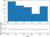 |
Fig. 7 Same as Fig. 6, but now phased to the rotation period of Prot = 0.514275 days. |
| In the text | |
|
Fig. 8 Cross-correlation between the different rotations of AB Dor TESS light curve, using the first observed rotation in the same data as a reference (see text for details). |
| In the text | |
|
Fig. 9 Rows 0, 300 and 600 of the autocorrelation functions Ak,j from the AB Dor light-curve; see text for details. |
| In the text | |
|
Fig. 10 Time-lag diagram of autocorrelation functions Ak,j. It is importantto note the decrease in correlation (see text for details). |
| In the text | |
|
Fig. 11 Mean autocorrelation as function of lag for the light curve of AB Dor; see text for details. |
| In the text | |
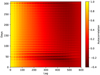 |
Fig. 12 Same as Fig. 10, but from our simulated light curve. |
| In the text | |
|
Fig. 13 Top panel: same as Fig. 11, but from our simulated light curve and assumed spot lifetime of 12 days. Middle and bottom panels: collapsed Aij from our simulated light curves for spots with assumed lifetimes of 6 and 24 days, respectively. |
| In the text | |
Current usage metrics show cumulative count of Article Views (full-text article views including HTML views, PDF and ePub downloads, according to the available data) and Abstracts Views on Vision4Press platform.
Data correspond to usage on the plateform after 2015. The current usage metrics is available 48-96 hours after online publication and is updated daily on week days.
Initial download of the metrics may take a while.