| Issue |
A&A
Volume 643, November 2020
|
|
|---|---|---|
| Article Number | A156 | |
| Number of page(s) | 14 | |
| Section | Atomic, molecular, and nuclear data | |
| DOI | https://doi.org/10.1051/0004-6361/202038909 | |
| Published online | 19 November 2020 | |
Theoretical investigation of oscillator strengths and lifetimes in Ti II⋆
1
Department of Materials Science and Applied Mathematics, Malmö University, 20506 Malmö, Sweden
e-mail: This email address is being protected from spambots. You need JavaScript enabled to view it.
2
Hebei Key Lab of Optic-electronic Information and Materials, The College of Physics Science and Technology, Hebei University, Baoding 071002, PR China
Received:
13
July
2020
Accepted:
27
September
2020
Abstract
Aims. Accurate atomic data for Ti II are essential for abundance analyses in astronomical objects. The aim of this work is to provide accurate and extensive results of oscillator strengths and lifetimes for Ti II.
Methods. The multiconfiguration Dirac–Hartree–Fock and relativistic configuration interaction (RCI) methods, which are implemented in the general-purpose relativistic atomic structure package GRASP2018, were used in the present work. In the final RCI calculations, the transverse-photon (Breit) interaction, the vacuum polarisation, and the self-energy corrections were included.
Results. Energy levels and transition data were calculated for the 99 lowest states in Ti II. Calculated excitation energies are found to be in good agreement with experimental data from the Atomic Spectra Database of the National Institute of Standards and Technology based on the study by Huldt et al. Lifetimes and transition data, for example, line strengths, weighted oscillator strengths, and transition probabilities for radiative electric dipole (E1), magnetic dipole (M1), and electric quadrupole (E2) transitions, are given and extensively compared with the results from previous calculations and measurements, when available. The present theoretical results of the oscillator strengths are, overall, in better agreement with values from the experiments than the other theoretical predictions. The computed lifetimes of the odd states are in excellent agreement with the measured lifetimes. Finally, we suggest a relabelling of the 3d2(12D)4p y2 D3/2o and z2 P3/2o levels.
Key words: atomic data
Full Table 3 is only available at the CDS via anonymous ftp to cdsarc.u-strasbg.fr (130.79.128.5) or via http://cdsarc.u-strasbg.fr/viz-bin/cat/J/A+A/643/A156
© ESO 2020
1. Introduction
Iron-group elements have high cosmic abundances and display, due to their complex atomic structure, rich spectra in astronomical objects. Titanium is among the lighter elements in this group and is identified as an α-element that is primarily produced by captures of He nuclei. Studies of metal-poor stars, aimed to probe early galactic chemical compositions, show correlations with abundances of scandium and vanadium and thus a common production route with the iron-group elements (Sneden et al. 2016).
Spectroscopic analyses of astronomical objects rely on accurate transition data for elemental abundances, which in turn are crucial input to stellar and galactic evolution modelling. Data that are needed include wavelengths and oscillator strengths as well as hyperfine structure. The current paper addresses this important need.
We note that Ti II is one of the most abundant ions and its lines are found in the ultraviolet, visible, and near-infrared spectra of B, A, and F stars, for example. Furthermore, its parity forbidden nebular lines are found in stellar winds (Ryde 2009; Cowan et al. 2020; Hartman et al. 2004).
The energy levels of Ti II presented in the Atomic Spectra Database (ASD) of the National Institute of Standards and Technology (NIST; see Kramida et al. 2019) were compiled by Sugar & Corliss (1985) and Saloman (2012) based on the results from Huldt et al. (1982). The observed spectral lines of Ti II were compiled from sources of Huldt et al. (1982), Allende Prieto & Garcia Lopez (1998), Pickering et al. (2001), and Aldenius (2009) for electric dipole (E1) transitions and of Hartman et al. (2004, 2005) and Bautista et al. (2006) for magnetic dipole (M1) and electric quadrupole (E2) transitions.
There are a number of experimental and theoretical studies of lifetimes and oscillator strengths of the Ti II ion. The sources adopted in the compilation by the NIST ASD are summarised in Table 1, and they include those of Roberts et al. (1973, 1975), Wolnik & Berthel (1973), Danzmann & Kock (1980), Kostyk & Orlova (1983), Pickering et al. (2001), Wiese et al. (2001), Morton (2003), Hartman et al. (2005), and Deb et al. (2008).
Summary of previous works on oscillator strengths and lifetimes in Ti II.
On the experimental side, a number of studies of lifetimes have been presented in the literature. Within the FERRUM project, Hartman et al. (2003) reported measurements of the long lifetime of the 3d2(3P)4s4P5/2 level in TiII, using the laser probing technique (LPT) (Lidberg et al. 1999) at the CRYRING storage ring (Abrahamsson et al. 1993). This measurement, however, resulted in a lifetime (28 ± 10 s) more than a factor of 2 longer than the theoretical estimate. The large uncertainty was due to the systematic effect of repopulation. Later on, within the same project, Hartman et al. (2005) extended the work on the measurement of lifetimes of other four metastable levels and determined the absolute transition probabilities for eight forbidden transitions originating from the levels 3d4s22D3/2, 5/2, using a combination of laboratory and astrophysical measurements. Lifetimes for metastable levels were measured using the LPT. Branching fractions from some of these levels were derived from Hubble Space Telescope/STIS spectra of Eta Carinae. With the development of methods to eliminate the repopulation effects, Palmeri et al. (2008) re-measured the lifetime of 3d2(3P)4s4P5/2 using the same technique at CRYRING and they determined a shorter lifetime (16 ± 2 s).
A number of other authors have measured the lifetimes of short-lived Ti II levels. Kwiatkowski et al. (1985), Bizzarri et al. (1993), and Langhans et al. (1995) performed the measurements using a laser-induced fluorescence (LIF) technique. Roberts et al. (1973) determined some lifetimes of Ti II levels using the beam-foil technique. These sources are also given in Table 1.
A frequently used method to determine transition probabilities or oscillator strengths for E1 transitions is to combine the lifetime for the upper level with branching fractions (BF). The lifetime can be measured using the LIF technique and the BF are determined from, for example, Fourier transform spectroscopy (FTS) of a laboratory light source. This approach has been adopted by Bizzarri et al. (1993), Pickering et al. (2001), Wood et al. (2013), and Lundberg et al. (2016) to derive absolute transitions probabilities. Wiese et al. (2001) measured the oscillator strengths for the Ti II vacuum ultraviolet (VUV) resonance transitions  at 191.0938 nm and
  at 191.0609 nm, using the high sensitivity absorption spectroscopy (HSAS) experiment.
There are a few theoretical works presenting lifetimes or radiative transition rates for the complex system of Ti II. Luke (1999) calculated transition rates for E1 transitions between the fine structure levels of the terms 3d24p {4Go, 4Fo, 2Fo, 2Do, 4Do, 2Go} to the levels of the ground term 3d24s4F by using a configuration interaction (CI) method. Bautista et al. (2006) carried out calculations of radiative transition rates and lifetimes for states belonging to the {3d24s, 3d3, 3d24p, 3d4s2} configurations using the AUTOSTRUCTURE package (Badnell 1986). However, some of the theoretical metastable lifetimes obtained significantly disagree with the earlier measurements (Hartman et al. 2003, 2005). Palmeri et al. (2008) presented theoretical lifetimes of 13 metastable levels, along with the transition probabilities for several decay channels from these metastable levels obtained from three pseudo-relativistic Hartree–Fock (HFR) calculations, that is, HFR(A), HFR(B), and HFR(C), using the Cowan code (Cowan 1981). Deb et al. (2008) performed calculations of E2 and M1 transition probabilities among all 37 even parity levels, using the CIV3 code of Hibbert (1975), together with a semi-empirical fine-tuning technique to reproduce the experimental energy separations.
More recently, calculations of oscillator strengths of radiative E1 transitions and lifetimes for odd-parity states have been performed using a semi-empirical method (Ruczkowski et al. 2014, 2016). Lundberg et al. (2016) report oscillator strengths as well as lifetimes for highly excited states from laboratory measurements and calculations. The calculations were carried out using the HFR method of Cowan (1981), taking core-polarisation effects into account.
Extensive calculations of energy levels, oscillator strengths, and lifetimes in Ti II were also carried out by Kurucz using the semi-empirical approach, and these data are available in Kurucz (2017). The oscillator strengths from Kurucz (2017) for strong lines are well known to agree rather well with experimental values, but for weak lines they are inevitably more uncertain.
In the present work, ab initio calculations were performed for the 99 (37 even and 62 odd) lowest states belonging to the even {3d24s, 3d3, 3d4s2} configurations and to the odd {3d24p, 3d4s4p} configurations in Ti II. The calculations were performed based on the fully relativistic multiconfiguration Dirac–Hartree–Fock (MCDHF) and relativistic configuration interaction (RCI) methods, as implemented in the newest version of the general-purpose relativistic atomic structure package GRASP2018 (Froese Fischer et al. 2019). Energy levels as well as E1, M1, and E2 transition data were computed along with the corresponding lifetimes of these states.
2. Multiconfiguration Dirac–Hartree–Fock approach
In the MCDHF method (Grant 2007; Froese Fischer et al. 2016), the atomic state functions (ASFs) used to describe the states of the atom are approximate eigenfunctions of the Dirac-Coulomb Hamiltonian given by
![Mathematical equation: $$ \begin{aligned} H_{\rm DC} = \sum _{i=1}^N [c{\boldsymbol{\alpha }}_i\cdot {\boldsymbol{{p}}}_i + ({\boldsymbol{\beta }}_i - 1)c^2 + V_i^N] + \sum _{i>j}^N \frac{1}{r_{ij}}, \end{aligned} $$](/articles/aa/full_html/2020/11/aa38909-20/aa38909-20-eq5.gif) (1)
(1)
where α and β are the 4 × 4 Dirac matrices,  is the monopole part of the electron–nucleus Coulomb interaction, c is the speed of light in atomic units, pi ≡ −i∇ is the electron momentum operator, and rij is the distance between electrons i and j. The ASFs (Ψ) are expanded over configuration state functions (CSFs, Φ):
 (2)
(2)
The CSFs are jj-coupled many-electron functions built from products of one-electron Dirac orbitals. As for the notation, J and M are the angular quantum numbers, P is parity, and γi specifies the occupied subshells of the CSF with their complete angular coupling tree information, including for instance the orbital occupancy, coupling scheme, and other quantum numbers necessary to uniquely describe the CSFs.
The radial parts of the Dirac orbitals together with the expansion coefficients ci of the CSFs are obtained in a relativistic self-consistent field (SCF) procedure by solving the Dirac–Hartree–Fock radial equations and the configuration interaction eigenvalue problem, resulting from applying the variational principle on the statistically weighted energy functional of the targeted states with terms added in order to preserve the orthonormality of the one-electron orbitals. The angular integrations needed for the construction of the energy functional are based on the second quantisation method in the coupled tensorial form (Gaigalas et al. 1997, 2001).
Higher order interactions, such as the transverse photon interaction and quantum electrodynamic effects (vacuum polarisation and self-energy), are added to the Dirac-Coulomb Hamiltonian in subsequent RCI calculations (McKenzie et al. 1980). Keeping the radial components from the previous step fixed, the expansion coefficients ci of the CSFs for the targeted states are obtained by solving the configuration interaction eigenvalue problem.
The transition data (e.g. transition probabilities and weighted oscillator strengths) between two states γ′P′J′ and γPJ are expressed in terms of reduced matrix elements of the transition operator T (Grant 1974):
 (3)
(3)
For E1 and E2 transitions, there are the following two forms of the transition operator: the Babushkin and Coulomb forms, which are equivalent to the length and the velocity form in the non-relativistic quantum mechanics. Babushkin and Coulomb gauges for the exact solutions of the Dirac-equation give the same value of the transition moment (Grant 1974).
3. Computational schemes
Calculations were performed in the extended optimal level (EOL) scheme (Dyall et al. 1989) for the weighted average of the even and odd parity states. These states belong to the {3d24s, 3d3, 3d4s2} even configurations and the {3d24p, 3d4s4p} odd configurations. From the initial calculations and analysis of the eigenvector compositions, we identified a number of configurations giving considerable contributions to the total wave functions. Particularly, the two-electron excitation configurations {3p43d44s, 3p43d34s2, and 3p43d5} are of crucial importance to predict the correct order of the energy levels for even states. These important configurations, together with the target configurations, define what is known as the multireference (MR). The MR sets for the even and odd parities are presented in Table 2, which also displays the number of CSFs in the final even and odd state expansions distributed over the different J symmetries.
Summary of the active space construction.
The CSF expansions were determined using the multireference-single-double (MR-SD) method, allowing single and double (SD) substitutions from configurations in the MR to orbitals in an active set (AS; Olsen et al. 1988; Sturesson et al. 2007; Froese Fischer et al. 2016). In the MCDHF calculations, no substitutions were allowed from the Ar-like core (1s22s22p63s23p6), which defines an inactive closed core. This means that only valence-valence (VV) electron correlation effects were taken into account in the MCDHF calculations. These calculations were followed by RCI calculations for an extended expansion, which was achieved by opening the 3s and 3p core shells for substitutions to include core-valence (CV) and core-core (CC) effects. In the RCI calculations, 1s22s22p6 was kept as an inactive closed core. The CV expansion was obtained by allowing SD substitutions from the valence orbitals and the 3s23p6 core, with the restriction that there was one substitution at most from 3s23p6 to the active set {8s, 8p, 8d, 8f, 8g, 8h, 7i}. The inclusion of CC correlations in the calculations decreases the excitation energies significantly and they also have large effects on the energy separations. Considering the fact that the inclusion of CC correlations increases the number of CSFs very rapidly, which is beyond the reach of the available computational resources, the CC expansion was obtained by allowing SD substitutions from both 3s and 3p shells to the active set {8s, 8p, 8d}. The MR set in the RCI calculations was extended to include additional important configurations. For these configurations, single substitutions from valence and core orbitals were allowed to the active orbital set {8s, 8p, 8d} and double substitutions to {4s, 4p, 4d}. The number of CSFs in the final even and odd state expansions are 14 089 101 and 15 573 967, respectively, and they are distributed over the different J symmetries.
4. Results and discussions
4.1. Energy levels
The energies and wave function composition in LS-coupling for the 99 (37 even and 62 odd) lowest states for Ti II are given in Table A.1. In the calculations, the labelling of the eigenstates is determined by the LSJ-coupled CSF with the largest coefficient in the expansion resulting from the transformation from jj-coupling to LSJ-coupling using the method by Gaigalas et al. (2017).
The accuracy of the wave functions from the present calculation was evaluated by comparing the calculated energy levels with experimental data from Huldt et al. (1982) provided via the NIST ASD. In most cases, the differences of the computed energy levels compared to the experimental data are less than 1.0%. The largest disagreements are for the 4F states in the ground configuration 3d24s and the first excited configuration 3d3, and the differences are about 4%. The averaged uncertainty of computed energy spectra compared to NIST data is 1.06%.
In addition, the Landé g-factors for the 99 states in Ti II were derived from the wave function expansions. The results were collected and made available in a recent paper by Li et al. (2020), in which they provide a collection of theoretical Landé g-factors for ions of astrophysical interest.
4.2. Transition rates and oscillator strengths
Transition data, for example, wavenumbers, wavelengths, line strengths, weighted oscillator strengths, as well as transition probabilities of E1, M1, and E2 transitions are given in Table 3; a full table is available at the CDS. We note that the wavenumbers and wavelengths are adjusted to match the level energy values in the NIST ASD.
Transition data of E1, M1, and E2 transitions for Ti II from the present calculations.
The uncertainties of the computed LS-allowed E1 transition rates can be estimated by the relative differences between values in length and velocity forms, dT (Froese Fischer 2009; Ekman et al. 2014):
 (4)
(4)
where Al and Av are the transition rates in length and velocity form. For all the strong E1 transitions with A ≥ 106 s−1, which are dominated by the LS-allowed transitions, dT always remains below 20%; the mean dT of these strong transitions is 0.122. Contrary to the strong transitions, 891 out of 1302 E1 transitions are weaker transitions with A < 106 s−1, which are associated with larger dT values; the average dT for these transitions is 0.509. These weak transitions are mainly LS-forbidden E1 transitions, for example, the intercombination and two-electron one-photon transitions. For these types of transitions, as discussed in Ekman et al. (2014), dT can no longer be used as an uncertainty estimate for each individual transition rate and it should only be used if averaging over a very large sample. On the other hand, the transitions are governed by the outer part of the wave functions; the length form is more sensitive to this part of the wave functions and it is generally considered to be the preferred form (Grant 1974; Hibbert 1974). Therefore, only transition data and lifetimes in length form are presented in this work.
The accuracy of calculated transition rates in length form can be estimated by extensive comparisons with other theoretical works and experimental results. In Fig. 1, log(g f) values from the present work are compared with available results from NIST ASD. The NIST data are compiled based on the results from Roberts et al. (1973, 1975), Wolnik & Berthel (1973), Danzmann & Kock (1980), Kostyk & Orlova (1983), Pickering et al. (2001), Wiese et al. (2001), and Morton (2003) for E1 transitions and from Hartman et al. (2005) and Deb et al. (2008) for M1 and E2 transitions. As shown in the figure, the agreement between the log(g f) values computed in the present work and the respective results from the NIST database are rather good for most of the transitions. Furthermore, the computed log(g f) values are compared with the results from various experimental sources (Blackwell et al. 1982; Bizzarri et al. 1993; Pickering et al. 2001, 2002; Wood et al. 2013), which were carried out by a combination of LIF and FTS methods, as seen in Figs. 2–5 in the left panels for the present work and the right panels for other recent theoretical results (Ruczkowski et al. 2014; Lundberg et al. 2016; Kurucz 2017). From the figures, we note an overall better agreement between the present results and experimental values, especially for transitions with log(g f) ≥ 1.0. The comparisons between other theoretical values, that is, semi-empirical calculations (Ruczkowski et al. 2014; Kurucz 2017) and HFR calculations (Lundberg et al. 2016) as well as experimental results show a much wider scatter.
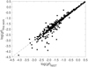 |
Fig. 1. Comparison of log(g f) values of the current study with the values available in the NIST ASD. |
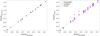 |
Fig. 2. Comparison of the theoretical log(g f) values to those published by Blackwell et al. (1982). Left panel: this work (black square). Right panel: Ruczkowski et al. (2014) (red square); Lundberg et al. (2016) (blue circle); and Kurucz (2017) (magenta triangle). |
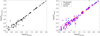 |
Fig. 3. Comparison of the theoretical log(g f) values to those published by Bizzarri et al. (1993). Left panel: this work (black square). Right panel: Ruczkowski et al. (2014) (red square); Lundberg et al. (2016) (blue circle); and Kurucz (2017) (magenta triangle). |
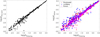 |
Fig. 4. Comparison of the theoretical log(g f) values to those published by Pickering et al. (2001, 2002). Left panel: this work (black square). Right panel: Ruczkowski et al. (2014) (red square); Lundberg et al. (2016) (blue circle); and Kurucz (2017) (magenta triangle). |
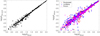 |
Fig. 5. Comparison of the theoretical log(g f) values to those published by Wood et al. (2013). Left panel: this work (black square). Right panel: Ruczkowski et al. (2014) (red square); Lundberg et al. (2016) (blue circle); and Kurucz (2017) (magenta triangle). |
In Table 4, the computed and measured log(g f) values for the two VUV resonance transitions are given. Wiese et al. (2001) measured the log(g f) values using the HSAS experiment at the Synchrotron Radiation Center in Stoughton, Wisconsin. Pickering et al. (2001) determined the two values by a combination of FTS branching fractions and Kurucz’s calculated lifetimes. The discrepancy between the values obtained from the two different methods are quite large for the 1910.954 Å transition, and the present computed value is in good agreement with the one from Wiese et al. (2001). We have revised the Pickering et al. (2001) data by combining their BFs with our lifetimes, which should be more accurate than previous calculations. The new data is included in the last column in Table 4. It can be seen that the new log(g f) values are in excellent agreement with those from Wiese et al. (2001).
Comparison between experimental and calculated oscillator strengths (log(g f)) for the VUV resonance transitions.
In addition, the present work can be compared with other theoretical calculations. In Fig. 6, log(g f) values from the present work are compared with the results from CI (Luke 1999) as well as semi-empirical (Ruczkowski et al. 2014; Kurucz 2017) and HFR (Lundberg et al. 2016) calculations, when available. As shown in the figure, the deviations between the log(g f) values computed in the present work and respective results from other sources are small for values down to −1.5, with a much wider scatter for the weaker lines. Given the overall good agreement between the present work and experimental results observed in the above mentioned discussions, we suggest that the current results together with the experimental values are used as a reference.
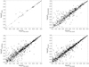 |
Fig. 6. Comparison of log(g f) values of the current study with the values from other theoretical work. Top left: Luke (1999). Top right: Ruczkowski et al. (2014). Bottom left: Lundberg et al. (2016). Bottom right: Kurucz (2017). |
For the M1 and E2 forbidden transitions, there are a number of measurements of transition rates A. In Table 5, the computed A values are compared with experimental results by Hartman et al. (2005), which were obtained using a combination of laboratory and astrophysical measurements. The computed A values from the present work and semi-empirical calculations from Kurucz’s database (Kurucz 2017) are in much better agreement with those measurements than from the other theoretical results, that is, the HFR calculation by Palmeri et al. (2008) and the CI calculation by Deb et al. (2008), which were compiled in the NIST ASD. Computed A values from the present work are within the uncertainties of experimental measurements, except for transitions 3d4s22D3/2 – 3d2(1D)4s2D3/2, 5/2, for which, on the contrary, the various theoretical works give much closer values. Finally, in Fig. 7, we compare the computed M1 and E2 transition rates with values from the CI calculations by Deb et al. (2008). As shown in the figure, the deviations are small for most of the strong transitions, but with a much wider scatter for the weaker lines.
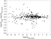 |
Fig. 7. Comparison of log(A) values for M1+E2 transitions between even states of the current study with the values from Deb et al. (2008). |
Comparison between experimental and calculated forbidden transition probabilities.
4.3. Lifetimes
The calculated lifetimes are compared with other theoretical predictions and experimental values, when available, in Tables A.2 and A.3 for even and odd states, respectively. The agreement with Kurucz’s semi-empirical results (Kurucz 2017) is overall good for both even and odd states.
In Fig. 8, the lifetimes from experiments (Palmeri et al. 2008; Hartman et al. 2003, 2005) using the LPT approach are compared with the results from the present calculations and from other theoretical works (Kurucz 2017; Deb et al. 2008; Palmeri et al. 2008; Grant 1974; Bautista et al. 2006). As can be seen from the figure, the theoretical values from this work fall into, or only slightly outside, the range of the estimated uncertainties of the experimental values. On the contrary, the differences between the measured and computed lifetimes by Deb et al. (2008), using the CIV3 code, are larger for all of these values.
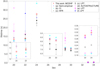 |
Fig. 8. Comparison of the experimental (with error bars) and calculated lifetimes (in s) for even states of Ti II. (a) Kurucz (2017); (b) Deb et al. (2008); (c) Palmeri et al. (2008); (d) Bautista et al. (2006); (e) Hartman et al. (2005); and (f) Hartman et al. (2003). We note that ilev, a label in the x-axis, corresponds to the ilev in Table A.1. |
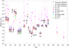 |
Fig. 9. Comparison of the experimental (with error bars) and calculated lifetimes (in ns) for odd states of Ti II. (a) Kurucz (2017); (b) Ruczkowski et al. (2016); (c) Bizzarri et al. (1993); (d) Kwiatkowski et al. (1985); (e) Roberts et al. (1973); (f) Langhans et al. (1995); (g) Gosselin et al. (1987); and (h) Lundberg et al. (2016). We note that ilev, a label in the x-axis, corresponds to the ilev in Table A.1. |
For odd states, a number of measurements of lifetimes (Roberts et al. 1973; Kwiatkowski et al. 1985; Gosselin et al. 1987; Bizzarri et al. 1993; Langhans et al. 1995; Lundberg et al. 2016) are compared with the theoretical results from the present work, semi-empirical calculations (Ruczkowski et al. 2016; Kurucz 2017), and HFR calculations (Lundberg et al. 2016). As shown in the figure, the measured lifetimes from Roberts et al. (1973) are overall larger than the values from other measurements, and all the calculated values from the present work agree with those of the latter within the experimental errors. The Kurucz’s values, which are frequently used as a reference in many literature, are in agreement with experimental values in most cases, except for the  ,
,  , and
, and  levels.
4.4. Labelling of the  and
and  levels
The NIST label classification for Ti II adheres to the analysis by Huldt et al. (1982), who assigned the 39 603 cm−1 level as  and the 39 233 cm−1 level as
  . Due to the strong mixing between the states, the assignment is uncertain and it was later questioned by Bizzarri et al. (1993). Based on lifetime measurements, they suggested that the assignments for the two levels should be interchanged. However, they did not update the identifications, according to their suggestion, and the lifetime values and oscillator strengths in later publications (Pickering et al. 2001, 2002; Wood et al. 2013) are presented using the original identification. The present calculations support the suggestion of Bizzarri. Our calculated level energies are 39 357 cm−1 for
  and 39 723 cm−1 for
  , suggesting the experimental level 39 233 cm−1 to be
  and the level 39 603 cm−1 to be
  . By reassigning the two levels, there is also a significant improvement in the agreement between our theoretical and the measured log(g f) values. As shown in Fig. 10, after correcting the labels, the agreement is very good for most of the transitions. Further support for the reassignment is offered by the lifetimes, which are 5.48 and 4.42 ns, respectively, for
  and
and  from the present work, relative to 4.5(2) and 5.5(3) ns from Bizzarri et al. (1993) using the original identifications. Again, the reassignment of the two levels results in a perfect agreement between the theoretical and measured lifetimes (see Table A.3). Please note that all the labels in this paper have been corrected to the new labels.
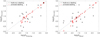 |
Fig. 10. Comparison of the theoretical log(g f) values for the transitions involving |
5. Summary and conclusions
In the present work, extended transition data of E1, M1, and E2 transitions and lifetimes are made available for Ti II using MCDHF and RCI methods. The computations of transition properties in the systems of Ti II are challenging, mainly due to the strong interaction between the terms and configurations of the even states. Thus, some of the states are strongly mixed, and highly correlated wave functions are needed to accurately predict their LS-composition. It is found that the inclusion of {3p43d44s, 3p43d34s2 and 3p43d5} configurations in MR is very important to predict the correct order of the even energy levels.
We have performed an extensive comparison of the computed oscillator strengths and lifetimes with other theoretical and experimental results. There is a significant improvement in the accuracy in the computed oscillator strengths of E1 transitions compared with previous theoretical works.
The computed lifetimes of odd states are all in excellent agreement with the measured lifetimes. We suggest that the current results be used as a reference for Ti II for various astrophysical applications.
A careful comparison of the energies of the levels, the oscillator strengths, as well as the radiative lifetimes with the experimental values has made possible the identification of the mislabelling of the  and
and  levels adopted in the NIST ASD. The assignments for the
  and
and  levels should be interchanged.
Acknowledgments
This work is supported by the Swedish research council under contracts 2015-04842 and 2016-04185. Kai Wang acknowledges the support from the National Natural Science Foundation of China (Grant No. 11703004), the Natural Science Foundation of Hebei Province, China (A2019201300), and the Natural Science Foundation of Educational Department of Hebei Province, China (BJ2018058). We would also like to thank the anonymous referee for her/his useful comments that helped improve the original manuscript.
References
- Abrahamsson, K., Andler, G., Bagge, L., et al. 1993, Nucl. Instrum. Methods Phys. Res. Sect. B: Beam Interact. Mater. At., 79, 269 [NASA ADS] [CrossRef] [Google Scholar]
- Aldenius, M. 2009, Phys. Scr., T134, 014008 [NASA ADS] [CrossRef] [Google Scholar]
- Allende Prieto, C., & Garcia Lopez, R. J. 1998, A&AS, 131, 431 [NASA ADS] [CrossRef] [EDP Sciences] [Google Scholar]
- Badnell, N. R. 1986, J. Phys. B: At. Mol. Phys., 19, 3827 [NASA ADS] [CrossRef] [Google Scholar]
- Bautista, M. A., Hartman, H., Gull, T. R., Smith, N., & Lodders, K. 2006, MNRAS, 370, 1991 [NASA ADS] [CrossRef] [Google Scholar]
- Bizzarri, A., Huber, M. C. E., Noels, A., et al. 1993, A&A, 273, 707 [NASA ADS] [Google Scholar]
- Blackwell, D. E., Menon, S. L. R., & Petford, A. D. 1982, MNRAS, 201, 603 [CrossRef] [Google Scholar]
- Cowan, R. D. 1981, The Theory of Atomic Structure and Spectra ((Berkeley, CA: University of California Press)) [Google Scholar]
- Cowan, J. J., Sneden, C., Roederer, I. U., et al. 2020, ApJ, 890, 119 [CrossRef] [Google Scholar]
- Danzmann, K., & Kock, M. 1980, J. Phys. B: At. Mol. Phys., 13, 2051 [NASA ADS] [CrossRef] [Google Scholar]
- Deb, N. C., Hibbert, A., Felfli, Z., & Msezane, A. Z. 2008, J. Phys. B: At. Mol. Opt. Phys., 42, 015701 [CrossRef] [Google Scholar]
- Dyall, K., Grant, I., Johnson, C., Parpia, F., & Plummer, E. 1989, Comput. Phys. Commun., 55, 425 [NASA ADS] [CrossRef] [Google Scholar]
- Ekman, J., Godefroid, M., & Hartman, H. 2014, Atoms, 2, 215 [NASA ADS] [CrossRef] [Google Scholar]
- Froese Fischer, C. 2009, Phys. Scr. Vol. T, 134, 014019 [NASA ADS] [CrossRef] [Google Scholar]
- Froese Fischer, C., Godefroid, M., Brage, T., Jönsson, P., & Gaigalas, G. 2016, J. Phys. B: At. Mol. Opt. Phys, 49, 182004 [NASA ADS] [CrossRef] [Google Scholar]
- Froese Fischer, C., Gaigalas, G., Jönsson, P., & Bieroń, J. 2019, Comput. Phys. Commun., 237, 184 [NASA ADS] [CrossRef] [Google Scholar]
- Gaigalas, G., Rudzikas, Z., & Froese Fischer, C. 1997, J. Phys. B At. Mol. Phys., 30, 3747 [NASA ADS] [CrossRef] [Google Scholar]
- Gaigalas, G., Fritzsche, S., & Grant, I. P. 2001, Comput. Phys. Commun., 139, 263 [NASA ADS] [CrossRef] [Google Scholar]
- Gaigalas, G., Froese Fischer, C., Rynkun, P., & Jönsson, P. 2017, Atoms, 5, 6 [NASA ADS] [CrossRef] [Google Scholar]
- Gosselin, R., Pinnington, E., & Ansbacher, W. 1987, Phys. Lett. A, 123, 175 [CrossRef] [Google Scholar]
- Grant, I. P. 1974, J. Phys. B: At. Mol. Opt. Phys, 7, 1458 [NASA ADS] [CrossRef] [Google Scholar]
- Grant, I. P. 2007, Relativistic Quantum Theory of Atoms and Molecules (New York: Springer) [CrossRef] [Google Scholar]
- Hartman, H., Rostohar, D., Derkatch, A., et al. 2003, J. Phys. B: At. Mol. Opt. Phys., 36, L197 [CrossRef] [Google Scholar]
- Hartman, H., Gull, T., Johansson, S., Smith, N., & Team, H. E. C. T. P. 2004, A&A, 419, 215 [NASA ADS] [CrossRef] [EDP Sciences] [Google Scholar]
- Hartman, H., Schef, P., Lundin, P., et al. 2005, MNRAS, 361, 206 [NASA ADS] [CrossRef] [Google Scholar]
- Hibbert, A. 1974, J. Phys. B: At. Mol. Phys., 7, 1417 [CrossRef] [Google Scholar]
- Hibbert, A. 1975, Comput. Phys. Commun., 9, 141 [NASA ADS] [CrossRef] [Google Scholar]
- Huldt, S., Johansson, S., Litzén, U., & Wyart, J.-F. 1982, Phys. Scr., 25, 401 [NASA ADS] [CrossRef] [Google Scholar]
- Kostyk, R. I., & Orlova, T. V. 1983, Astrometriia i Astrofizika, 49, 39 [Google Scholar]
- Kramida, A., Ralchenko, Y., Reader, J., & NIST ASD Team 2019, NIST Atomic Spectra Database (ver. 5.7.1) (Gaithersburg, MD: National Institute of Standards and Technology), https://physics.nist.gov/asd [2020, May 13] [Google Scholar]
- Kurucz, R. L. 2017, On-line Database of Observed and Predicted Atomic Transitions (Cambridge, MA: Harvard-Smithsonian Center for Astrophysics), http://kurucz.harvard.edu [Google Scholar]
- Kwiatkowski, M., Werner, K., & Zimmermann, P. 1985, Phys. Rev. A, 31, 2695 [CrossRef] [Google Scholar]
- Langhans, G., Schade, W., & Helbig, V. 1995, Z. Phys. D At. Mol. Clusters, 34, 151 [CrossRef] [Google Scholar]
- Li, W., Rynkun, P., Radžiūtė, L., et al. 2020, A&A, 639, A25 [CrossRef] [EDP Sciences] [Google Scholar]
- Lidberg, J., Al-Khalili, A., Norlin, L. O., et al. 1999, Nucl. Instrum. Methods Phys. Res. Sect. B: Beam Interact. Mater. At., 152, 157 [NASA ADS] [CrossRef] [Google Scholar]
- Luke, T. M. 1999, Can. J. Phys., 77, 571 [CrossRef] [Google Scholar]
- Lundberg, H., Hartman, H., Engström, L., et al. 2016, MNRAS, 460, 356 [NASA ADS] [CrossRef] [Google Scholar]
- McKenzie, B. J., Grant, I. P., & Norrington, P. H. 1980, Comput. Phys. Commun., 21, 233 [NASA ADS] [CrossRef] [Google Scholar]
- Morton, D. C. 2003, ApJS, 149, 205 [NASA ADS] [CrossRef] [MathSciNet] [Google Scholar]
- Morton, D. C. 2004, ApJS, 151, 403 [NASA ADS] [CrossRef] [Google Scholar]
- Olsen, J., Roos, B. O., Jørgensen, P., & Jensen, H. J. A. 1988, J. Chem. Phys., 89, 2185 [NASA ADS] [CrossRef] [Google Scholar]
- Palmeri, P., Quinet, P., Biémont, É., et al. 2008, J. Phys. B: At. Mol. Opt. Phys., 41, 125703 [NASA ADS] [CrossRef] [Google Scholar]
- Pickering, J. C., Thorne, A. P., & Perez, R. 2001, ApJS, 132, 403 [NASA ADS] [CrossRef] [Google Scholar]
- Pickering, J. C., Thorne, A. P., & Perez, R. 2002, ApJS, 138, 247 [NASA ADS] [CrossRef] [Google Scholar]
- Roberts, J. R., Andersen, T., & Sorensen, G. 1973, ApJ, 181, 567 [NASA ADS] [CrossRef] [Google Scholar]
- Roberts, J. R., Voigt, P. A., & Czernichowski, A. 1975, ApJ, 197, 791 [CrossRef] [Google Scholar]
- Ruczkowski, J., Elantkowska, M., & Dembczynski, J. 2014, J. Quant. Spectrosc. Radiat. Transfer, 149, 168 [CrossRef] [Google Scholar]
- Ruczkowski, J., Elantkowska, M., & Dembczynski, J. 2016, J. Quant. Spectrosc. Radiat. Transfer, 176, 6 [CrossRef] [Google Scholar]
- Ryde, N. 2009, Physica Scripta, T134, 014001 [CrossRef] [Google Scholar]
- Saloman, E. B. 2012, J. Phys. Chem. Ref. Data, 41, 013101 [NASA ADS] [CrossRef] [Google Scholar]
- Savanov, I. S., Huovelin, J., & Tuominen, I. 1990, A&AS, 86, 531 [NASA ADS] [Google Scholar]
- Sneden, C., Cowan, J. J., Kobayashi, C., et al. 2016, ApJ, 817, 53 [NASA ADS] [CrossRef] [Google Scholar]
- Sturesson, L., Jönsson, P., & Froese Fischer, C. 2007, CoPhC, 177, 539 [Google Scholar]
- Sugar, J., & Corliss, C. 1985, J. Phys. Chem. Ref. Data, 14, 2 [Google Scholar]
- Thevenin, F. 1989, A&AS, 77, 137 [NASA ADS] [Google Scholar]
- Wiese, L. M., Fedchak, J. A., & Lawler, J. E. 2001, ApJ, 547, 1178 [NASA ADS] [CrossRef] [Google Scholar]
- Wolnik, S. J., & Berthel, R. O. 1973, ApJ, 179, 665 [CrossRef] [Google Scholar]
- Wood, M. P., Lawler, J. E., Sneden, C., & Cowan, J. J. 2013, ApJS, 208, 27 [NASA ADS] [CrossRef] [Google Scholar]
Appendix A: Atomic state function composition in LS-coupling, energy levels, and lifetimes for the Ti II ion.
Atomic state function composition (up to three LS components with a contribution >0.02 of the total wave function) in LS-coupling and energy levels (in cm−1) for Ti II.
Comparison of the experimental (with the uncertainty in the last digit given in parentheses) and calculated lifetimes (in s) for even states of Ti II.
Comparison of the experimental (with the uncertainty in the last digit given in parentheses) and calculated lifetimes (in ns) for odd states of Ti II.
All Tables
Transition data of E1, M1, and E2 transitions for Ti II from the present calculations.
Comparison between experimental and calculated oscillator strengths (log(g f)) for the VUV resonance transitions.
Comparison between experimental and calculated forbidden transition probabilities.
Atomic state function composition (up to three LS components with a contribution >0.02 of the total wave function) in LS-coupling and energy levels (in cm−1) for Ti II.
Comparison of the experimental (with the uncertainty in the last digit given in parentheses) and calculated lifetimes (in s) for even states of Ti II.
Comparison of the experimental (with the uncertainty in the last digit given in parentheses) and calculated lifetimes (in ns) for odd states of Ti II.
All Figures
|
Fig. 1. Comparison of log(g f) values of the current study with the values available in the NIST ASD. |
| In the text | |
|
Fig. 2. Comparison of the theoretical log(g f) values to those published by Blackwell et al. (1982). Left panel: this work (black square). Right panel: Ruczkowski et al. (2014) (red square); Lundberg et al. (2016) (blue circle); and Kurucz (2017) (magenta triangle). |
| In the text | |
|
Fig. 3. Comparison of the theoretical log(g f) values to those published by Bizzarri et al. (1993). Left panel: this work (black square). Right panel: Ruczkowski et al. (2014) (red square); Lundberg et al. (2016) (blue circle); and Kurucz (2017) (magenta triangle). |
| In the text | |
|
Fig. 4. Comparison of the theoretical log(g f) values to those published by Pickering et al. (2001, 2002). Left panel: this work (black square). Right panel: Ruczkowski et al. (2014) (red square); Lundberg et al. (2016) (blue circle); and Kurucz (2017) (magenta triangle). |
| In the text | |
|
Fig. 5. Comparison of the theoretical log(g f) values to those published by Wood et al. (2013). Left panel: this work (black square). Right panel: Ruczkowski et al. (2014) (red square); Lundberg et al. (2016) (blue circle); and Kurucz (2017) (magenta triangle). |
| In the text | |
|
Fig. 6. Comparison of log(g f) values of the current study with the values from other theoretical work. Top left: Luke (1999). Top right: Ruczkowski et al. (2014). Bottom left: Lundberg et al. (2016). Bottom right: Kurucz (2017). |
| In the text | |
|
Fig. 7. Comparison of log(A) values for M1+E2 transitions between even states of the current study with the values from Deb et al. (2008). |
| In the text | |
|
Fig. 8. Comparison of the experimental (with error bars) and calculated lifetimes (in s) for even states of Ti II. (a) Kurucz (2017); (b) Deb et al. (2008); (c) Palmeri et al. (2008); (d) Bautista et al. (2006); (e) Hartman et al. (2005); and (f) Hartman et al. (2003). We note that ilev, a label in the x-axis, corresponds to the ilev in Table A.1. |
| In the text | |
|
Fig. 9. Comparison of the experimental (with error bars) and calculated lifetimes (in ns) for odd states of Ti II. (a) Kurucz (2017); (b) Ruczkowski et al. (2016); (c) Bizzarri et al. (1993); (d) Kwiatkowski et al. (1985); (e) Roberts et al. (1973); (f) Langhans et al. (1995); (g) Gosselin et al. (1987); and (h) Lundberg et al. (2016). We note that ilev, a label in the x-axis, corresponds to the ilev in Table A.1. |
| In the text | |
|
Fig. 10. Comparison of the theoretical log(g f) values for the transitions involving |
| In the text | |
Current usage metrics show cumulative count of Article Views (full-text article views including HTML views, PDF and ePub downloads, according to the available data) and Abstracts Views on Vision4Press platform.
Data correspond to usage on the plateform after 2015. The current usage metrics is available 48-96 hours after online publication and is updated daily on week days.
Initial download of the metrics may take a while.