| Issue |
A&A
Volume 643, November 2020
|
|
|---|---|---|
| Article Number | A33 | |
| Number of page(s) | 10 | |
| Section | Galactic structure, stellar clusters and populations | |
| DOI | https://doi.org/10.1051/0004-6361/202038885 | |
| Published online | 27 October 2020 | |
Orbit classification in a disk galaxy model with a pseudo-Newtonian central black hole
1
Department of Physics, School of Science, Aristotle University of Thessaloniki, 541 24 Thessaloniki, Greece
e-mail: This email address is being protected from spambots. You need JavaScript enabled to view it.
2
Facultad de Ciencias Humanas y de la Educación, Universidad de los Llanos, Villavicencio, Colombia
e-mail: This email address is being protected from spambots. You need JavaScript enabled to view it.
3
Academic Department of Mathematics, Universidade Tecnológica Federal do Paraná (UTFPR), Av. Sete de Setembro, 3165 Curitiba, Brazil
e-mail: This email address is being protected from spambots. You need JavaScript enabled to view it.
4
Nonlinear Analysis and Applied Mathematics (NAAM)-Research Group, Department of Mathematics, Faculty of Science, King Abdulaziz University, PO Box 80203, Jeddah 21589, Saudi Arabia
Received:
9
July
2020
Accepted:
31
August
2020
Abstract
We numerically investigate the motion of stars on the meridional plane of an axially symmetric disk galaxy model, containing a central supermassive black hole, represented by the Paczyński-Wiita potential. By using this pseudo-Newtonian potential we can replicate important relativistic properties such as the existence of the Schwarzschild radius. After classifying extensive samples of initial conditions of trajectories, we managed to distinguish between collisional, ordered, and chaotic motion. Besides all starting conditions of regular orbits were further classified into families of regular orbits. Our results are presented via color-coded basin diagrams on several types of two-dimensional planes. Our analysis reveals that both the mass of the black hole (in direct relation with the Schwarzschild radius) as well as angular momentum play an important role in the character of the orbits of stars. More specifically, the trajectories of low angular momentum stars are highly affected by the mass of the black hole, while high angular momentum stars seem to be unaffected by the central black hole. A comparison with previous related outcomes, using Newtonian potentials for the central region of the galaxy, is also made.
Key words: galaxies: kinematics and dynamics / galaxies: structure / chaos
© ESO 2020
1. Introduction
Galactic dynamics is of paramount importance not only because of the evident astronomical interest in classifying and analyzing the nature of galaxies (Binney & Tremaine 2008; Manos & Athanassoula 2011; Zotos 2012), but also to investigate the nature of dark matter that constitutes a significant part of these objects (Zotos & Caranicolas 2013). Exploring the nature of orbits using different models of galaxies can provide a hint about the nature of dark matter present in these structures. Moreover, the phase space structure of a particular model depends on its basic components, that is, the disk, halo, and nucleus or central bulge (Zotos 2012, 2014; Zotos & Carpintero 2013), such that its phase space is as unique as a fingerprint. In general terms, orbits can be classified according to their dynamical behavior into regular and chaotic (Caranicolas 1996; Caranicolas & Papadopoulos 2003; Zotos 2012, 2014; Zotos & Carpintero 2013). Regular orbits can be subclassified into different families depending on the resonances of the individual orbits (Martinet & Mayer 1975; Manabe 1979; Greiner 1987; Lees & Schwarzschild 1992), which can be analyzed using different techniques (Binney & Spergel 1982, 1984; Laskar 1993; Carpintero & Aguilar 1998; Zotos & Carpintero 2013). This analysis in essence decomposes a trajectory function into its constituent frequencies. Also, it is important to note that a typical galaxy has billions of stars, making simulations computationally expensive, therefore several analytical models are proposed based on Newtonian theory and general relativity.
In Newtonian theory, globular and spherical galaxies are represented by the popular models of Plummer (Plummer 1911) and King (King 1966). Highly flattened axisymmetric galaxies are usually modeled by the so-called Toomre model (Toomre 1963), while thickened disks are modeled by Miyamoto and Nagai potentials (Miyamoto & Nagai 1975). The Miyamoto-Nagai model is a stationary and axially symmetric potential, which despite the deviations in its density profile in comparison with realistic models provides a simple and reasonable model for a disk. Concerning the galactic nuclei, most of the analytical models are spherical with finite masses, while the isotropic velocity dispersion can be calculated analytically (see, e.g., Jaffe 1983; de Zeeuw 1985; Hernquist 1990; Zhao 1996). Newtonian models for massive black hole nuclei have been also proposed aiming to reproduce the final stage for the evolution of active galactic nuclei (Rees 1984) or to realistically mimic the nuclei of galaxies (Häring & Rix 2004). The linearity of Newtonian equations allows for the superposition of different models to study, for example, galactic models composed of a disk and a bulge (Binney & Tremaine 2008).
In addition to the well-known spherical solutions, in general relativity several exact disk-like solutions have been proposed to model galaxies, including static thin disks (Bonnor & Sackfield 1968; Morgan & Morgan 1969; Ujevic & Letelier 2004) and thick disks (González & Letelier 2004). To obtain these models it is usual to start with the metric and calculate the energy momentum from the metric. A different approach uses the energy-momentum tensor as a source of Einstein’s equations but this is highly nontrivial. In the framework of general relativity, the composition of different models is not always possible owing to the nonlinearity of the Einstein equations. Nevertheless, there are some special cases where the superposition of exact solutions is possible (Lemos & Letelier 1993; Semerak 2002, 2004). A review of these and other relativistic models can be found in Semerak (2002) and Vogt & Letelier (2005).
There is compelling evidence of supermassive black holes in the center of several galaxies, including the Milky Way (Liu et al. 2019), where general relativity is found to provide a natural scenario for its study. On the other hand, Newtonian models are computationally cheaper and can be easily built and analyzed. A balance between the two extremes can be achieved using Newtonian equations that include pseudo-potentials that reproduce some relativistic effects. In particular, some of the most renowned pseudo-Newtonian potentials have originally been introduced to study accretion disks in black holes (Paczyński & Wiita 1980; Semerak & Karas 1999). The simplest and at the same time practical of these potentials is that derived by Paczyński and Wiita (Paczyński & Wiita 1980), which can correctly reproduce the locations of both the marginally bounded circular orbit and the last stable circular orbit of the Schwarzschild metric (Abramowicz 2009).
It is a well-known fact that pseudo-Newtonian potentials can have a remarkable effect on the dynamics of different systems (Steklain & Letelier 2006; Dubeibe et al. 2017; Zotos & Steklain 2019; Zotos et al. 2019). Therefore, in this paper we use the pseudo-Newtonian Paczyński-Wiita potential (Paczyński & Wiita 1980) to model the central part of a galaxy hosting a supermassive black hole, while the flat thin disk is represented by the Miyamoto-Nagai potential. Aiming to obtain direct outcomes on how the mimicked relativistic properties of the supermassive black hole affect the character of the trajectories of the stars, we study the influence of the Schwarzschild radius and the angular momentum of a test particle on the orbit classification, that is, collisional, ordered, and chaotic. With this approach, we are able to obtain direct outcomes on how the relativistic properties of the supermassive black hole (such as the Schwarzschild radius) affect the character of the trajectories of the stars, by comparing results from previous works (see, e.g., Zotos 2014; Zotos & Carpintero 2013), where the central nucleus was modeled by using a simple Newtonian Plummer potential (Plummer 1911). Regular and chaotic orbits are identified using the Smaller Alignment Index (SALI) method introduced by Skokos et al. (2004), while regular orbits are further classified into families of regular orbits (Carpintero & Aguilar 1998; Zotos & Carpintero 2013).
The article is structured as follows: in Sect. 2 we present the main properties of the galaxy model. In the following Sect. 3 we explain the computational methods we use for obtaining the classification of the orbits, which is presented in Sect. 4. Our article ends with Sect. 5, in which we emphasize the main outcomes of our analysis.
2. Description of the galaxy model
Our galaxy model describes the motion of stars on the meridional (R, z) plane and consists of two components. The first component is a flat thin disk represented by the Miyamoto-Nagai potential (Miyamoto & Nagai 1975) as
 (1)
(1)
where Md, k, and s are the mass, scale length and scale height of the disk, respectively.
For the description of the central black hole, we used the Paczyński-Wiita potential (see, e.g., Paczyński & Wiita 1980; Abramowicz 2009).
 (2)
(2)
where Mbh is the mass of the black hole. This is a very simple and practical pseudo-Newtonian potential, which however can realistically replicate and model the effects of general relativity, associated with the motion of test particles around a non-spinning black hole. Moreover, the Paczyński-Wiita potential alters the classical Newtonian potential 1/r to 1/(r − rs), thus introducing the relativistic Schwarzschild radius rs.
Because the total potential Φt(R, z) = Φd + Φbh has an axial symmetry, we have the conservation of the z-component (Lz) of the total angular momentum. This automatically implies that the motion of the test particle can be described using the effective potential
 (3)
(3)
and the set of the following equations of motion:
 (4)
(4)
 (5)
(5)
The energy integral of the system is given through the Hamiltonian
 (6)
(6)
where E is the test particle’s conserved value of the total orbital energy. We note that the test particle can access those areas of the phase space where E ≥ Φeff.
In our computations we used a system of units in which the unit of length is 1 kpc, the unit of time is 106 yr (1 Myr), the unit of mass is 2.22508 × 10¹¹ M⊙, the velocity unit is 978.564 km s−1, the angular momentum unit (per unit mass) is 978.564 km kpc−1 s−1, and the unit of energy (per unit mass) is 9.576 × 10⁵ km2 s−2. Then for the gravitational constant we have that G = 1. In the above units the values of the constant parameters are Md = 0.5 (corresponding to about 1011 M⊙), k = 3, and s = 0.175. On the other hand, the parameters Lz and Mbh are treated as free parameters.
The Schwarzschild radius is related to the mass of the black hole through the relation
 (7)
(7)
In the adopted system of galactic units, the value of the speed of light is roughly equal to 300 velocity units. Moreover, the values of the mass of the central black hole lie in the interval [108 M⊙, 1010 M⊙], which is a typical range of values in disk galaxies (Binney & Tremaine 2008). Consequently, from Eq. (7) we derive that the values of the Schwarzschild radius lie in the interval [10−8, 10−6]. However, such low values certainly induce computational malfunctions, since almost all numerical integrators cannot cope with motion extremely close to the singularity1. On this basis, to eliminate all ill behaviors during the numerical integration, we define a close encounter radius Rc around the singularity as Rc = 103rs. At this point, it should be noted that although there are some studies in which the motion of test particles can reach a closer position to the galactic center (see, e.g., Sukova & Semerak 2013), in the current study the close encounter radius does not affect the orbital dynamics of the test particle because the numerical artifact solely stops the numerical integration. Therefore in practice, the direct effect of this close encounter is the loss of information in the basin diagrams around the origin in a disk on the order of [10−5, 10−3] units of length for Mbh = [108 M⊙, 1010 M⊙], respectively.
In Zotos et al. (2018) we show that as long as rs > 0 there exists an additional energetically forbidden circular region around the black hole. Furthermore, the radius of the circular region is equal to the Schwarzschild radius. This begs the question whether the test particle is always able to reach the central black hole. The answer is no. Whether the test particle can approach the Schwarzschild radius or not strongly depends on the value of its angular momentum. More precisely, if its angular momentum is low enough then it can approach the Schwarzschild radius of the black hole and display a collision event. On the other hand, if its angular momentum is relatively high then it can never reach the boundaries of the black hole. In panel a of Fig. 1, we present the first case, in which the approach to the central black hole is possible. In this case, the zero-velocity curves (ZVCs), defined as Φeff(R, z) = E, are open, thus allowing the test particle to approach the black hole. In panel b of the same figure, we see the case in which the test particle cannot reach the central region of the galaxy. This is because in this case the ZVCs are closed, thus acting as potential barriers. In Fig. 2 we show the regions of open and closed ZVCs, as a function of (Lz, Mbh).
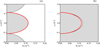 |
Fig. 1. Geometry of the zero velocity curves (black lines), near the central region of the galaxy, for Mbh = 0.05 and (a): Lz = 0.1, (b): Lz = 0.5. The energetically allowed and forbidden regions of motion are indicated using white and gray, respectively, while the red line corresponds to the Schwarzschild radius. |
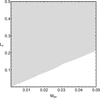 |
Fig. 2. White areas correspond to open ZVCs, where collision to the central black hole is possible, while gray areas denote closed ZVCs, where the test particle is not energetically allowed to approach the Schwarzschild radius. |
3. Computational methodology
Our work aims to determine how the mass Mbh of the black hole, along with the value of the angular momentum Lz, affects the character of motion of the test particles. For this task, we performed an orbit classification, by numerically integrating sets of 1024 × 1024 initial conditions of orbits. In all cases, the value of the total orbital energy is fixed to E = −0.05, which corresponds to the maximum possible value of R coordinate (about 10 kpc for a typical disk galaxy (see, e.g., Binney & Tremaine 2008)). We decided to keep the value of the energy fixed because its influence on the character of orbits moving in the meridional plane has already been revealed in Zotos (2016).
All initial conditions of the trajectories were numerically integrated for 104 time units, which correspond to about 1 Hubble time (14 billion years) while using a constant time step equal to 10−3. During the numerical integration, we also computed SALI (Skokos 2001), so as to be able to distinguish between chaotic and regular motion. This method allows us to classify the orbits according to the numerical value obtained after evolving two orthonormal deviation vectors w1 and w2, which are periodically normalized to prevent overflow errors. More precisely, if SALI > 10−4 the orbit is categorized as regular, while if SALI < 10−8 it is classified as chaotic; if the result belongs to the interval 10−4< SALI < 10−8, it is classified as sticky and the orbit requires a longer time of integration to be classified2. The index is formally defined as SALI ≡ min(d−,d+), where
 (8)
(8)
Once an orbit was classified as a regular one, then we performed an additional categorization, thus classifying regular initial conditions into regular families. Our analysis indicates that several types of regular orbits appear in our disk galaxy model, while the most important orbits are as follows: (i) box orbits; (ii) 1:1 orbits; (iii) 2:1 orbits; (iv) 2:3 orbits; (v) 4:3 orbits; and (vi) higher resonant orbits. Specifically, in all studied cases, the relative percentage of higher resonant orbits is always less than 0.1% and therefore we may argue that these orbits do not have any significant contribution to the overall orbital dynamics of the galaxy. The notation of orbits (box orbits and n : m resonant orbits) in the axially symmetric galaxy model is according to the initial works of Carpintero & Aguilar (1998) and Zotos & Carpintero (2013). In panels a–e of Fig. 3 we provide the shapes of the main regular orbits of the system, while in panel f of the same figure we give an example of a typical chaotic orbit when Mbh = 0.05. In all cases, the ZVC is the black thick curve circumscribing the orbits. For all regular types of trajectories, we tried to present regular orbits with starting conditions very close to the respective parent periodic orbits in order to be able to clearly recognize their shapes.
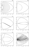 |
Fig. 3. Collection showing the most important types of motion, when Mbh = 0.05. (a): box orbit; (b): 2:1 orbit; (c): 1:1 orbit; (d): 2:3 orbit; (e): 4:3 orbit; (f): chaotic orbit. |
A double-precision Bulirsch-Stoer integrator, written in FORTRAN 77 (e.g., Press et al. 1992), was applied for the numerical integration of the starting conditions of the trajectories. During the numerical integration, the total energy of the test particle was sufficiently conserved, while the corresponding observed error was on the order of 10−14. For the classification of the initial conditions (per grid), the required CPU time, using a Quad-Core Intel i7 4.0 GHz processor, varied between 5 and 22 hours, strongly depending on the number of collision orbits. Version 12.1 of Mathematica® software (Wolfram 2003) was deployed to develop all the graphical illustrations of the article.
4. Orbit classification
In this section, we present the nature of the motion of the test particle as a function of the mass of the black hole and the angular momentum. To illustrate the orbital properties of the galactic system, hereafter we follow the graphical approach introduced in Nagler (2004, 2005), thus presenting color-coded basin diagrams, in which each pixel corresponds to a unique trajectory and is colored according to the final state of the test particle.
All trajectories have initial conditions (R0, z0), while for a given total orbital energy E0 the initial velocities are given by
 (9)
(9)
 (10)
(10)
where
 (11)
(11)
while  .
.
4.1. Low angular momentum
We begin our analysis, considering the case in which the test particle (star) takes low values of the angular momentum. In Figs. 4a–b we present the basin diagrams on the (R, z) plane, when Lz = 0.001. We only consider z > 0 because the axial symmetry of the galaxy causes the orbital structure of z < 0 to be mirror symmetrical. Panel a corresponds to the case in which the mass of the black hole is Mbh = 0.0005. The first type of motion that we encounter as we move away from the center are box orbits. There are two main basins occupied by initial conditions of box orbits, while between these basins we have the presence of the 2:1 resonant orbits. Both basins of box orbits are “polluted” by a mixture of chaotic and collision orbits, while tiny stability islands of higher resonant orbits are also present. We observe the presence of 2:1 and 1:1 resonant orbits very close to the boundaries of the ZVC, while there are no signs of other resonant orbits such as 4:3.
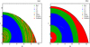 |
Fig. 4. Basin diagrams on the (R, z) plane for Lz = 0.001, where (a): Mbh = 0.0005 and (b): Mbh = 0.05. |
The case with Mbh = 0.05 is shown in panel b of Fig. 4. We see that the pollution of collision orbits shown in panel a is much stronger leading to well-defined basins of collision. Inside the collision basin near the central black hole, we observe the presence of a stability island corresponding to 1:1 resonant orbits. On the other hand, higher resonant orbits seem to be completely absent for this value of Mbh. Moreover, all initial conditions belonging to chaotic orbits (according to the value of SALI) lead, sooner or later, to a collision with the central black hole, and therefore there are no remaining trapped chaotic trajectories.
In order to illustrate the difference between the two cases regarding the collision orbits more clearly, we present in Figs. 5a–b the distributions of the corresponding collision times of the trajectories. In panel a, corresponding to Mbh = 0.0005 we see that the vast majority of the starting conditions need a significant amount of time (more than 2500 time units) to reach the central black hole. However, we distinguish some very thin basins of initial conditions for which the corresponding collision time is very low (less than 300 time units). On the other hand, in panel b of Fig. 5 we see that almost all the initial conditions lead to a collision with the black hole within the first 1000 time units of the numerical integration. Therefore, we may reasonably ask why the orbits collide so quickly in the second case. Fortunately, the answer is very easy. In both cases, the ZVCs are open near the center and therefore the test particle can approach the central black hole. The main difference is that in the second case (where Mbh = 0.05) the Schwarzschild radius is 100 times larger, which implies that the collision channel is much wider. Consequently, the test particles need significantly less time to find the open throat and collide with the singularity.
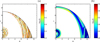 |
Fig. 5. Distribution of the collision times for Lz = 0.001, where (a): Mbh = 0.0005 and (b): Mbh = 0.05. |
4.2. Intermediate angular momentum
The second case under investigation concerns test particles moving with intermediate values of angular momentum. The basin diagrams on panels a and b of Fig. 6 show the orbital structure of the meridional (R, z) plane, when Lz = 0.1. Panel a corresponds to Mbh = 0.0005. We see that collision motion is not possible. This is also seen in the diagram of Fig. 2, where we can extract the valuable information that for (Mbh, Lz) = (0.0005, 0.1) the corresponding ZVCs are closed. We may argue that for this set of values of Mbh and Lz almost the entire (R, z) plane is covered by box and 2:1 orbits, while all other types of orbits are extremely limited or even absent.
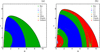 |
Fig. 6. Basin diagrams on the (R, z) plane for Lz = 0.1, where (a): Mbh = 0.0005 and (b): Mbh = 0.05. |
For a much higher value of the mass of the black hole, we see in panel b of Fig. 6 that extended collision basins emerge close and far from the central singularity, thus leading to a considerable reduction of the area corresponding to box orbits. Moreover, we can see that now the test particle can also perform 1:1 and 4:3 resonant orbits.
4.3. High angular momentum
The last scenario under consideration is the case with high angular momentum stars. Figures 7a–b show the basins diagrams on the (R, z) plane, when Lz = 0.5. Now we observe that the value of the mass of the black hole only affects resonant orbits. This implies that high angular momentum stars, moving on box and 2:1 orbits are hardly affected by the central black hole. Furthermore, this type of star cannot even approach the singularity, taking into account that for such high values of the angular momentum the ZVCs are always closed, thus not allowing collision with the black hole. Another interesting fact is that the 1:1 and 2:3 resonant types of motion seem to be more prominent, compared to all other previous cases, while on the other hand, the 4:3 resonant orbits are barely noticeable. Moreover, it should be noted that with increasing value of the angular momentum, while keeping constant the value of the total orbital energy, the energetically allowed region on the meridional (R, z) plane is considerably reduced.
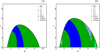 |
Fig. 7. Basin diagrams on the (R, z) plane for Lz = 0.5, where (a): Mbh = 0.0005 and (b): Mbh = 0.05. |
4.4. Overview analysis
It would be very informative to present the influence of the angular momentum Lz as well as of the mass of the black hole Mbh on the nature of the motion of the test particles from another perspective. In Figs. 8a–b we present the character of the trajectories, with initial conditions on the (R, Lz) plane, while for all orbits we set z0 = 0. It is seen that when the value of the mass of the black hole is low, collision orbits are very limited and appear only for very low values of the angular momentum (Lz < 0.01), that is, when stars can approach very close to the galactic center. On the other hand, when Mbh is high enough collision is still possible, even for relatively large angular momentum values (Lz < 0.1). Box orbits occupy most of the (R, Lz) plane, while the second most populated type of motion is the 2:1 resonant family, which lies around 4–5 kpc. Furthermore, we can see that for Mbh = 0.05, the 4:3 resonant orbits appear at about Lz = 0.1, while the 2:3 resonant orbits exist mainly for Lz > 0.2. Isolated initial conditions of higher resonant orbits can be observed scattered inside the area of box orbit.
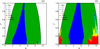 |
Fig. 8. Basin diagrams on the (R, Lz) plane, where (a): Mbh = 0.0005 and (b): Mbh = 0.05. |
The parametric evolution of the percentages of all the main types of orbits, as a function of the angular momentum, is given in panels a and b of Fig. 9. This figure shows that the orbital content of the system is affected by the value of the mass of the black hole mainly for low values of the angular momentum (Lz < 0.2), while for higher values the pattern is almost unaffected by the shift on the value of Mbh. We also see that for large angular momentum values (Lz → 1) box orbits completely dominate, while at the same time resonant orbits, such as the 2:3 and 4:3 orbital families, disappear.
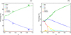 |
Fig. 9. Evolution of the percentages of all main types of orbits on the (R, Lz) plane, as a function of the angular momentum, when (a): Mbh = 0.0005 and (b): Mbh = 0.05. |
Before concluding, we would like to present some additional information regarding the collision time of the trajectories and the connection between the angular momentum and the mass of the black hole. In Fig. 10 we show the evolution of the average collision of orbits as a function of the angular momentum for three values of Mbh. We see that the average collision time is reduced, with increasing value of the mass of the black hole. Moreover, in all three cases, the collision time increases, with increasing value of the angular momentum, and tends to the total time of the numerical integration (104 time units). This is anticipated because with an increasing value of Lz the width of the collision channel of the ZVCs, near the galactic center, is reduced. The vertical red dashed lines indicate the maximum values of the angular momentum for which a collision is possible; evidently, for higher values of Lz the corresponding ZVCs are closed. We would also like to note that these critical values of the angular momentum, obtained through the numerical integration, coincide with the respective values obtained earlier (see Fig. 2) using analytical methods.
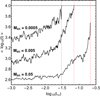 |
Fig. 10. Evolution of the average collision time of the trajectories, with initial conditions on the (R, Lz) plane, as a function of the angular momentum. The horizontal black dashed line indicates the total time of the numerical integration, while the vertical red dashed lines denote the maximum value of Lz, for which the ZVCs are open. |
5. Concluding remarks
In this work, we numerically investigated the motion of stars on the meridional (R, z) plane of an axially symmetric disk galaxy model, containing a central supermassive black hole. To model the black hole we used the Paczyński-Wiita potential, which can replicate important relativistic properties such as the existence of the Schwarzschild radius rs. After classifying extensive samples of initial conditions of trajectories, we managed to distinguish between collisional, ordered, and chaotic motion. Furthermore, all starting conditions of regular orbits are further classified into families of regular orbits. Our results are presented through modern color-coded basin diagrams on several types of two-dimensional planes, while we also monitored the evolution of the respective percentages.
The following list summarizes the main outcomes, regarding the motion of stars:
-
We have seen that the parameters of both the angular momentum and the mass of the black hole determine if the stars are able to approach the central singularity or not. In general terms, open ZVCs (which allow collision with the black hole) are present only when Lz < 0.2.
-
For low values of the angular momentum, only the most basic types of orbits exist (such as box, 1:1, and 2:1), while higher resonant orbits (such as the 2:3 and 4:3 orbital families) appear only for higher values of the Lz.
-
For relatively low values of the mass of the black hole (Mbh ≃ 0.0005) we encountered the phenomenon of trapped chaos, where chaotic orbits remained trapped inside the ZVCs for at least one Hubble time, even though collision to the central black hole is energetically allowed. On the other hand, for high values of Mbh, there is no evidence of trapped chaos and all chaotic orbits lead fast to a collision.
-
Low angular momentum stars (with Lz < 0.1) are highly affected by the mass of the black hole. More specifically, for low values of Mbh they can either move on a box, 2:1, or chaotic orbit, while a collision is less possible. On the contrary, for high values of Mbh the possibility of collision is much higher, while regular motion seems to be shared between box and 2:1 types of orbits.
-
High angular momentum stars (with Lz > 0.5) seem to be less affected by the value of the mass of the black hole since they cannot even approach the central regions of the galaxy. Our analysis indicates that the vast majority of high angular momentum stars move either on box or 2:1 trajectories.
In two earlier works (Zotos 2014; Zotos & Carpintero 2013) we also investigated the nature of motion in a disk galaxy model using the same Miyamoto-Nagai model. However, the central nucleus was modeled with a typical Plummer potential (Plummer 1911), while in the present study we use a pseudo-Newtonian Paczyński-Wiita potential (Paczyński & Wiita 1980). Therefore, we can directly compare the differences between the classical Newtonian and the pseudo-Newtonian models. In both cases, the main types of regular orbits are the same, while the influence of the angular momentum seems to be similar. In particular, we see that high angular momentum stars move mainly on regular orbits, while low angular momentum stars can display chaotic motion, by passing close to the central region. The main difference between the two cases is the fact that in the case of the Plummer potential we encountered additional types of resonant orbits (e.g., 5:4 and 6:5). Thus, we may argue that in the pseudo-Newtonian case of the Paczyński-Wiita potential the orbital content of regular motion is not as rich as in the case of the Plummer potential. Additionally, in the case of the Plummer potential several types of resonant orbits, such as 2:3, 4:3, 5:4, and 6:5, were simultaneously present. On the contrary, in the case of the Paczyński-Wiita potential, we observe a hierarchy regarding the appearance of resonant orbits. Specifically, for low values of Lz we have the presence of the 4:3 orbits, while the 2:3 orbits appear for much higher values of the angular momentum. Finally, for the Newtonian case of the Plummer potential we encounter many more types of higher resonant orbits n : m (with n, m > 5) inside the area of the box orbits, while in the case of the Paczyński-Wiita potential all these higher resonant orbits are completely absent.
Consequently, we believe that our findings can be relevant not only from a theoretical point of view but also from an astrophysical perspective. In particular, the identification of resonant orbits could shed lights on the formation and origin of kinematic moving groups (Martinez-Medina et al. 2016), while the presence of chaotic or collisional orbits could certainly modify the structure and hence the evolution of the galaxy with the increase of the central black hole mass. Taking into account the positive and encouraging results of the present analysis, we plan to expand our orbit classification into three dimensions. We would aim to determine how the mass of the black hole in combination with the angular momentum of the stars affects their trajectories inside three-dimensional (x, y, z) space. Moreover, it would also be interesting to determine the influence of the mass of the black hole on the network of periodic orbits of the galaxy.
Our previous experience indicates that the Bulirsch-Stoer integrator we used in our study can adequately follow the evolution of a test particle up to a radius equal to 10−5 around the singularity, while for smaller radii it displays several well-known malfunctions such as time step “overflow”.
Skokos (2001) provides a detailed explanation of the method.
Acknowledgments
This project was funded by the Deanship of Scientific Research (DSR) at King Abdulaziz University, Jeddah, Saudi Arabia, under Grant no. KEP-42-130-38. The authors, therefore, acknowledge with thanks DSR technical and financial support. F. L. D. acknowledges financial support from the Universidad de los Llanos. Our warmest thanks go to the anonymous referee for the careful reading of the manuscript as well as for all the apt suggestions and comments, which allowed us to improve both the quality and the clarity of the paper.
References
- Abramowicz, M. A. 2009, A&A, 500, 213 [NASA ADS] [CrossRef] [EDP Sciences] [Google Scholar]
- Binney, J., & Spergel, D. 1982, ApJ, 252, 308 [NASA ADS] [CrossRef] [Google Scholar]
- Binney, J., & Spergel, D. 1984, MNRAS, 206, 159 [NASA ADS] [Google Scholar]
- Binney, J., & Tremaine, S. 2008, Galactic Dynamics (Princeton, USA: Princeton Univ. Press) [Google Scholar]
- Bonnor, W. B., & Sackfield, A. 1968, Commun. Math. Phys., 8, 338 [CrossRef] [Google Scholar]
- Carpintero, D. D., & Aguilar, L. A. 1998, MNRAS, 298, 1 [NASA ADS] [CrossRef] [Google Scholar]
- Caranicolas, N. D. 1996, Astrophys. Space Sci., 246, 15 [NASA ADS] [CrossRef] [Google Scholar]
- Caranicolas, N. D., & Papadopoulos, N. J. 2003, A&A., 399, 957 [CrossRef] [Google Scholar]
- de Zeeuw, T. 1985, MNRAS, 216, 273 [NASA ADS] [CrossRef] [Google Scholar]
- Dubeibe, F. L., Lora-Clavijo, F. D., & González, G. A. 2017, Phys. Lett. A, 381, 563 [CrossRef] [Google Scholar]
- González, G. A., & Letelier, P. S. 2004, Phys. Rev. D., 69, 044013 [CrossRef] [Google Scholar]
- Greiner, J. 1987, Celest. Mech., 40, 171 [CrossRef] [Google Scholar]
- Häring, N., & Rix, H. W. 2004, ApJ, 604, L89 [NASA ADS] [CrossRef] [Google Scholar]
- Hernquist, L. 1990, ApJ, 356, 359 [Google Scholar]
- Jaffe, W. 1983, MNRAS, 202, 995 [NASA ADS] [Google Scholar]
- King, I. R. 1966, AJ, 71, 64 [Google Scholar]
- Laskar, J. 1993, Phys. D: Nonlinear Phenom., 67, 257 [NASA ADS] [CrossRef] [Google Scholar]
- Lees, J. F., & Schwarzschild, M. 1992, ApJ, 384, 491 [NASA ADS] [CrossRef] [Google Scholar]
- Lemos, J. P. S., & Letelier, P. S. 1993, Class. Quant. Grav., 10, 6 [CrossRef] [MathSciNet] [Google Scholar]
- Liu, J., Zhang, H., Howard, A. W., et al. 2019, Nature, 575, 7784 [Google Scholar]
- Manos, T., & Athanassoula, E. 2011, MNRAS, 415, 1 [NASA ADS] [CrossRef] [Google Scholar]
- Manabe, S. 1979, PASJ, 31, 369 [NASA ADS] [Google Scholar]
- Martinet, L., & Mayer, F. 1975, A&A, 44, 45 [Google Scholar]
- Martinez-Medina, L. A., Pichardo, B., Moreno, E., Peimbert, A., & Velazquez, H. 2016, ApJ, 817, L3 [NASA ADS] [CrossRef] [Google Scholar]
- Morgan, T., & Morgan, L. 1969, Phys. Rev., 183, 5 [CrossRef] [Google Scholar]
- Miyamoto, M., & Nagai, R. 1975, PASJ, 27, 533 [NASA ADS] [Google Scholar]
- Nagler, J. 2004, Phys. Rev. E, 69, 066218 [NASA ADS] [CrossRef] [EDP Sciences] [Google Scholar]
- Nagler, J. 2005, Phys. Rev. E, 71, 026227 [NASA ADS] [CrossRef] [Google Scholar]
- Paczyński, B., & Wiita, P. J. 1980, A&A, 88, 23 [Google Scholar]
- Plummer, H. C. 1911, MNRAS, 71, 5 [Google Scholar]
- Press, H. P., Teukolsky, S. A., Vetterling, W. T., & Flannery, B. P. 1992, Numerical Recipes in FORTRAN 77, 2nd edn. (Cambridge: Cambridge University Press) [Google Scholar]
- Rees, M. J. 1984, ARA&A, 22, 471 [NASA ADS] [CrossRef] [Google Scholar]
- Semerak, O. 2002, Following the Prague Inspiration, to Celebrate the 60th Birthday of Jiri Bicák (Singapore: World Scientific) [Google Scholar]
- Semerak, O. 2004, Class. Quant. Grav., 21, 2203 [NASA ADS] [CrossRef] [Google Scholar]
- Semerak, O., & Karas, V. 1999, A&A, 343, 2 [Google Scholar]
- Skokos, C. 2001, J. Phys. A, 34, 10029 [NASA ADS] [CrossRef] [MathSciNet] [Google Scholar]
- Skokos, C., Antonopoulos, C., Bountis, T. C., & Vrahatis, M. N. 2004, J. Phys. A: Math. Gen., 37, 6269 [NASA ADS] [CrossRef] [MathSciNet] [Google Scholar]
- Steklain, A. F., & Letelier, P. S. 2006, Phys. Lett. A, 352, 4 [CrossRef] [Google Scholar]
- Sukova, P., & Semerak, O. 2013, MNRAS, 436, 978 [CrossRef] [Google Scholar]
- Toomre, A. 1963, ApJ, 138, 385 [NASA ADS] [CrossRef] [Google Scholar]
- Ujevic, M., & Letelier, P. S. 2004, Phys. Rev. D, 70, 8 [NASA ADS] [CrossRef] [Google Scholar]
- Vogt, D., & Letelier, P. S. 2005, MNRAS, 363, 1 [CrossRef] [Google Scholar]
- Wolfram, S. 2003, The Mathematica Book, 5th edn. (Champaign: Wolfram Media) [Google Scholar]
- Zhao, H. 1996, MNRAS, 278, 488 [Google Scholar]
- Zotos, E. E. 2012, New Astron., 17, 6 [NASA ADS] [CrossRef] [Google Scholar]
- Zotos, E. E. 2014, Mech. Res. Commun., 62, 102 [CrossRef] [Google Scholar]
- Zotos, E. E. 2016, Balt. Astron., 25, 139 [Google Scholar]
- Zotos, E. E., & Caranicolas, N. D. 2013, A&A, 560, A110 [NASA ADS] [CrossRef] [EDP Sciences] [Google Scholar]
- Zotos, E. E., & Carpintero, D. D. 2013, Celest. Mech. Dyn. Astron., 116, 417 [NASA ADS] [CrossRef] [Google Scholar]
- Zotos, E. E., & Steklain, A. F. 2019, Astrophys. Space Sci., 364, 10 [CrossRef] [Google Scholar]
- Zotos, E. E., Dubeibe, F. L., & González, G. A. 2018, MNRAS, 477, 5388 [CrossRef] [Google Scholar]
- Zotos, E. E., Dubeibe, F. L., Nagler, J., & Tejeda, E. 2019, MNRAS, 487, 2340 [CrossRef] [Google Scholar]
All Figures
|
Fig. 1. Geometry of the zero velocity curves (black lines), near the central region of the galaxy, for Mbh = 0.05 and (a): Lz = 0.1, (b): Lz = 0.5. The energetically allowed and forbidden regions of motion are indicated using white and gray, respectively, while the red line corresponds to the Schwarzschild radius. |
| In the text | |
|
Fig. 2. White areas correspond to open ZVCs, where collision to the central black hole is possible, while gray areas denote closed ZVCs, where the test particle is not energetically allowed to approach the Schwarzschild radius. |
| In the text | |
|
Fig. 3. Collection showing the most important types of motion, when Mbh = 0.05. (a): box orbit; (b): 2:1 orbit; (c): 1:1 orbit; (d): 2:3 orbit; (e): 4:3 orbit; (f): chaotic orbit. |
| In the text | |
|
Fig. 4. Basin diagrams on the (R, z) plane for Lz = 0.001, where (a): Mbh = 0.0005 and (b): Mbh = 0.05. |
| In the text | |
|
Fig. 5. Distribution of the collision times for Lz = 0.001, where (a): Mbh = 0.0005 and (b): Mbh = 0.05. |
| In the text | |
|
Fig. 6. Basin diagrams on the (R, z) plane for Lz = 0.1, where (a): Mbh = 0.0005 and (b): Mbh = 0.05. |
| In the text | |
|
Fig. 7. Basin diagrams on the (R, z) plane for Lz = 0.5, where (a): Mbh = 0.0005 and (b): Mbh = 0.05. |
| In the text | |
|
Fig. 8. Basin diagrams on the (R, Lz) plane, where (a): Mbh = 0.0005 and (b): Mbh = 0.05. |
| In the text | |
|
Fig. 9. Evolution of the percentages of all main types of orbits on the (R, Lz) plane, as a function of the angular momentum, when (a): Mbh = 0.0005 and (b): Mbh = 0.05. |
| In the text | |
|
Fig. 10. Evolution of the average collision time of the trajectories, with initial conditions on the (R, Lz) plane, as a function of the angular momentum. The horizontal black dashed line indicates the total time of the numerical integration, while the vertical red dashed lines denote the maximum value of Lz, for which the ZVCs are open. |
| In the text | |
Current usage metrics show cumulative count of Article Views (full-text article views including HTML views, PDF and ePub downloads, according to the available data) and Abstracts Views on Vision4Press platform.
Data correspond to usage on the plateform after 2015. The current usage metrics is available 48-96 hours after online publication and is updated daily on week days.
Initial download of the metrics may take a while.