| Issue |
A&A
Volume 643, November 2020
|
|
|---|---|---|
| Article Number | A157 | |
| Number of page(s) | 9 | |
| Section | Interstellar and circumstellar matter | |
| DOI | https://doi.org/10.1051/0004-6361/202038594 | |
| Published online | 18 November 2020 | |
The dipper light curve of V715 Persei: is there dust in the magnetosphere?
1
Departamento de Astronomía, Universidad de Guanajuato,
Callejón de Jalisco S/N,
Guanajuato,
Gto,
36240, México
e-mail: This email address is being protected from spambots. You need JavaScript enabled to view it.
2
Univ. Grenoble Alpes, CNRS, IPAG,
38000
Grenoble, France
Received:
5
June
2020
Accepted:
2
October
2020
Abstract
Context. The dipper optical light curves in young stellar objects are commonly interpreted as partial or total occultation of the stellar radiation by dust surrounding the star.
Aims. In this work, we analyze the amplitude of the optical light curve of V715 Per, located in the young star forming region IC 348. Observations gathered over the years suggest that the light curve can be explained by dust extinction events.
Methods. In our model, the dust is distributed inside the magnetosphere according to the strength of the stellar magnetic field. The dust distribution is modulated by the vertical component of the field whose axis is misaligned with respect to the rotational axis. We include a model for evaporation of the dust reaching the magnetosphere in order to consistently calculate its distribution.
Results. For V715 Per, there is dust in the optically thick warp at the disk truncation radius. We suggest that the optical light curve is explained by extinction caused by dust reaching inside the magnetosphere. The dust distribution is optically thin, and it cannot survive for a long time because of the high temperature and low density. However, as the grains rapidly move towards the stellar surface and the sublimation is not instantaneous, there is a layer of dust covering the magnetosphere responsible for the extinction.
Conclusions. Dust surviving the harsh conditions of the magnetospheric accretion flow may be responsible for some of the dipper light curves.
Key words: accretion, accretion disks / circumstellar matter
© ESO 2020
1 Introduction
The study of optical and near-infrared light curves of young stellar objects (YSOs) provides information about the distribution of dust surrounding them. Observed light curves of YSOs clearly show its variability (Alencar et al. 2010; Cody et al. 2014; Morales-Calderón et al. 2011; Stauffer et al. 2015, 2016); the different features allow different classes to be defined, demonstrating the rich and complex dynamics occurring in the dusty disk. For the modeling of light curves showing periodicity of a few days, it is required to take into account the interaction of the magnetic field lines defining the stellar magnetosphere with the inner edge of the disk, in particular for dipper light curves. The magneto-hydrodynamical simulations by Romanova et al. (2013) show the formation of magnetospheric streams and a bending wave in the innermost disk regions. These time-dependent structures with variable height can be used to interpret the light curves.
For a YSO, the optical flux mainly comes from the star, and therefore its variability either comes from changes of the spot distribution at the stellar surface or results from extinction of the stellar light by circumstellar dust. Here, we analyze the second mechanism in an attempt to directly extract the characteristics of the azimuthal dust distribution from the shape of the light curve. If the structures blocking the stellar radiation are optically thick, the color calculated between two optical wavelengths is constant in terms of phase. An object that has shown this kind of behavior in the past is AA Tau, whose light curve can be interpreted with a nonaxisymmetric optically thick warp in the innermost regions of the disk surrounding the star (Bouvier et al. 1999). These latter authors suggest that the warp is formed at the base of the magnetospheric streams caused by an inclined stellar magnetic field interacting with the disk. This idea was followed by others: Fonseca et al. (2014) studied V354 Mon, McGinnis et al. (2015) applied this to a large sample in NGC 2264, and Nagel & Bouvier (2019) studied the objects Mon-660, Mon-811, Mon-1140, and Mon-1308. The optical light curves analyzed in these works come from the CoRoT Space Telescope. Simultaneous observations with the Spitzer Space Telescope in the infrared allow a connect to be made between the behavior in both wavelength ranges, interpreted via the dust distributed around the star (McGinnis et al. 2015; Nagel & Bouvier 2019).
The YSO V715 Per is one of several objects that present light curves showing color changes consistent with circumstellar extinction (Barsunova et al. 2013, 2015, 2016). This behavior is common in young UX Ori stars; one of the main characteristics of this type is stochastic brightness variations caused by extinction where the dust is located in the circumstellar environment. Grinin et al. (2018) analyze V715 Per in the same way as in their previous works, where for five objects coming from a large set of T Tauri stars, the light curves can be explained by extinction (Barsunova et al. 2013, 2015, 2016). Also, Sicilia-Aguilar et al. (2020) show that the quasi-periodic eclipses in the young dipper RXJ1604.3-2130A can be explained with extinction at the base of the magnetospheric streams.
The stellar parameters of V715 Per are listed in Table 1. The first value for the stellar mass (M⋆) comes from Kirk & Myers (2011) and the one in parenthesis comes from LeBlanc et al. (2011). The values are different because LeBlanc et al. (2011) use the pre-main-sequence evolutionary models calculated by D’Antona & Mazzitelli (1997) while Kirk & Myers (2011) use the evolutionary tracks by Baraffe et al. (1998). The difference also depends on the way the bolometric luminosity Lbol is calculated because besides the spectral type, the value found by LeBlanc et al. (2011) uses the J-band magnitude and that by Kirk & Myers (2011) uses the estimated age of the object (1 Myr). The stellar radius (R⋆) is from LeBlanc et al. (2011) and the stellar effective temperature (T⋆) is taken from Luhman et al. (2003) using the associated spectral type (K6) shown in Herbig (1998). The mass accretion rate (Ṁ) is taken from Dahm (2008) where we take the mean of the values associated to the estimates using the HeI, Hα, and CaII lines. We remove the estimate using the R-band veiling because as mentioned in Dodin et al. (2012), if the veiling by lines is included, the depth changes vary for different photospheric lines such that the estimate of Ṁ is not reliable in this case. Ruiz-Rodriguez et al. (2018) observed the system with ALMA but the result was a nondetection, preventing them from deriving an inclination for the system.
The aim of this paper is to present a model to explain the amplitude and period of the optical light curve of V715 Per presented by Grinin et al. (2018). In our model, the variation of the magnitude comes from phase-dependent extinction due to material located in the magnetospheric streams.
In Sect. 2 we describe the characteristics of the optical light curve of V715 Per, in Sect. 3 we show the relevant aspects of the modeling, and in Sect. 4 we address two important questions, namely whether there is dust in the disk and whether there is dust in the magnetosphere. The free and fixed parameters of the model are described inSect. 5, and in Sect. 6 the model is applied to V715 Per. Finally, in Sect. 7 we present the conclusions of this study.
2 The characteristics of the periodic light curve of V715 Per
Grinin et al. (2018) present observations of the stellar system V715 Per in the optical (VRI bands) and in the infrared (JHK bands). These latter authors present photometric data compiled from different campaigns between 2003 and 2017, and for this long timescale they confirm the presence of low-amplitude periodic brightness variations of Δmag ~ 0.1 with a period equal to 5.25 days. Flaherty et al. (2013) photometrically studied this system with the Spitzer Space Telescope at 3.6 and 4.5 μm over 40 days and detected a signal with a period of 14.7days, which is not the stellar rotation period. The Keplerian radius corresponding to 5.25 days is 0.0574 AU. The bending wave formed by the hydrodynamical interaction of the stellar magnetic dipolar field and the gaseous disk (Romanova et al. 2013) is used for the physical interpretation of the data presented in Grinin et al. (2018). Because of the larger period, the IR light curve cannot be analyzed with the model used here, and therefore another mechanism is required to explain the photometric Spitzer data (Flaherty et al. 2013) for this system. The aim of this work is to explain the amplitude of the optical light curve. The interpretation of its details requires full 3D-MHD simulations taking into account each scenario in a highly dynamical region, and is well beyond the scope of this work.
In Grinin et al. (2018), the observed period in the light curve of P = 5.25 days is interpreted by occultations of material located at the Keplerian radius consistent with P. At this location, these latter authors assume that the material accreting radially in the disk is halted by the magnetic pressure associated with the stellar magnetic field. The stellar magnetic field is hereafter referred to as B. In other words, this radius also corresponds to the magnetospheric radius (Rmag) such that the occulting material belongs to the base of the magnetospheric streams near the plane of the disk that transport material towards the stellar surface at the magnetic poles, where two hot spots are formed.
3 The model used to interpret the observations
3.1 The system geometry and physical mechanisms
The period of 5.25 days is the one we are trying to interpret. A model consistent with this period involves material close to the star. The dust responsible for producing the stellar eclipses accretes in the disk reaching the outskirts of the magnetosphere located at the radius Rmag. The existence of dust inside the magnetosphere requires that the sublimation radius (Rsub) is smaller than Rmag. The disk regions close to the midplane are optically thick to the stellar radiation, and they are therefore responsible for producing total or partial stellar eclipses. For the well-known system AA Tau, the photometric data shaping the periodical optical light curve do not show color changes (Bouvier et al. 1999), and therefore the dust responsible for the shaping should be optically thick, whichis in accordance with an optically thick disk. For V715 Per, the periodic brightness variations show color changes consistent with circumstellar extinction, and therefore this material should be located in an optically thin environment. For the model presented here, this region corresponds to the dust located in the magnetospheric streams. We note that the radial dust distribution is not important for this estimate because the matter is added along the line of sight (LOS).
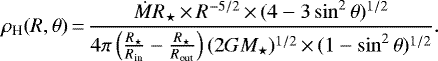
We use the model for accretion along a noninclined dipolar B presented in Hartmann et al. (1994) where the density is given by
 (1)
(1)
Here, G is the gravitational constant, R is the spherical radius, θ is the poloidal angle, and Rin and Rout correspond to the inner and outer intersections of the magnetospheric stream with the disk plane. We fix these values as Rin = 0.9Rmag and Rout = Rmag, as an order of magnitude estimate motivated by the simulations presented in Fig. 8 of Romanova et al. (2013). When used in the code, we take into account the fact that the dipole is inclined with respect to the rotational axis. As in Hartmann et al. (1994), the material velocity corresponds to ballistic infall from rest following the B lines. Finally, the gas density inside the magnetosphere (ρmag) is given by
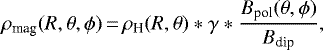 (2)
(2)
where ϕ is the azimuthal angle, Bpol is the poloidal magnetic field and B at R⋆ is given by Bdip. This factor is included in order to modulate the density such that the gas is concentrated where the magnetic pressure is larger. The value for the free-adimensional parameter γ is such that ρmag is consistent with Ṁ. Because the magnetic axis is inclined with respect to the rotational axis, Bpol depends on ϕ and θ. Taken together, this means that the gas distribution depends on the azimuthal (ϕ) and poloidal angles (θ) such that the optical depth varies for different LOSs. The presence and amount of dust is estimated using the temperature calculated as an equilibrium between the heating of stellar radiation and cooling as a blackbody at such a temperature. Two facts guarantee the presence of dust in the magnetosphere: (1) the grains do not sublimate instantaneously and (2) the free-fall time (tff) is just a few hours. This means that the dust can survive in a layer with an outer radius given by Rmag, and its inner boundary depends on the timescale of sublimation (tsub) and tff. In our modeling, the amount of dust in this layer is responsible for the deepness of the light curve at the various phases, as described in Sect. 6.
Parameters for V715 Per.
3.2 Details of the code used
According to a dust distribution around the star, the code calculates the total or partial extinction of the stellar radiation moving toward the observer. For our particular aim, the dust is located inside the magnetosphere, which is limited by Rmag. The dust reservoir is the protoplanetary disk where the grains are slowly moving towards the star. At Rmag, the material finds a radial equilibrium because the magnetic pressure is equal to the ram pressure, such that the vertical direction is the only available path to follow. As we are assuming that gas ionization is enough for the particles to be frozen to the B-lines, then the gas and the dust attached will follow the path given by the B-lines almost perpendicularly to the midplane of the disk. The material leaving the disk forms the magnetospheric streams which consist of B-lines that shrink as B is increased when it approaches the stellar surface. This behavior is taken into account to calculate the expression for ρmag (see Eq. (2)).
We assume that B is given by a dipolar magnetic field which is tilted with respect to the rotational axis by an angle βdip (Gregory et al. 2010)with B at R⋆ given by Bdip. In order to find Bdip, we use Eq. (1) in Konigl (1991) substituting the values for Rmag, M⋆, and Ṁ. For the model presented here, βdip = 5 deg and Bdip = 398 G. Along with βdip and Bdip, the longitude where the magnetic axis is tilted (ψdip) is the other free parameter that defines the stellar B. Because the star is azimuthally rotating, every section of the stellar surface crosses the LOS once every rotating period, which according to the modeling is equal to P. This means that the value ψdip is only relevant to locate the magnetic structure with respect to the light curve phases without changing the shape of the latter.
4 Presence of dust
4.1 Is there dust in the disk at Rmag?
For the stellar radiation that does not show color changes as in AA-Tau (Bouvier et al. 1999), the occulting structure should be optically thick. For the stellar system modeled here, this corresponds to the optically thick disk that is perturbed in the vertical direction to form the required structures according to each case. In this section, we answer the question, is there optically thick dust at Rmag for the stellar system V715 Per?
We use the stellar and disk parameters associated to this object (Grinin et al. 2018) shown in Table 1 to calculate the disk surface density:
![Mathematical equation: \begin{equation*} \Sigma\,{=}\,{\dot{M}\over 3\pi\alpha}{\Omega\mu m_{\textrm{H}}\over KT_{\textrm{c}}}[1-\sqrt{R_{\star}/R}] ,\end{equation*}](/articles/aa/full_html/2020/11/aa38594-20/aa38594-20-eq3.png) (3)
(3)
given by Lynden-Bell & Pringle (1974) for a viscous stationary disk. The viscosity is parameterized with α (we assume α = 0.01 as typical), Ω is the Keplerian angular velocity, μ is the molecular number, mH is the hydrogen mass, K is the Boltzmann constant, Tc is the temperature at the midplane, and R is the distance towards the star.
Using Σ, we calculate the disk density at Rmag with
 (4)
(4)
where H = cs∕Ω is the hydrostatic scale height and  is the sound speed. This results in
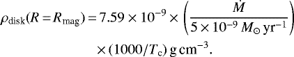 (5)
(5)
Using a linear interpolation of the Table 3 of Pollack et al. (1994) showing the sublimation temperature (Tsub) in terms of ρdisk, we estimate Tsub = 1417 K at R = Rmag. We use Ṁ = 5 × 10⁻⁹ M⊙ yr−1 and Tc = 1000 K as typical for the disk.
The temperature in the warp (Tmag = Tc(Rmag)) is calculatedusing the model of an optically thick wall heated by the stellar radiation presented in D’Alessio et al. (2005) and used in Nagel et al. (2010) to calculate the emission of the wall heated by a binary stellar system. For the stellar parameters given in Table 1, a typical dust composition, and a grain size distribution proportional to the power-law s−3.5 between a minimum grain size smin = 0.005 μm (according to the value used to characterize the interstellar medium (ISM); Mathis et al. 1977) and a maximum grain size smax = 1 mm (assuming that in the disk the grains increase in size from smax = 0.25 typical of the ISM), Tmag = 1309 K. As Tmag ≤ Tsub, we concludethat the warp does indeed contain dust, such that the assumption of an optically thick structure is valid. We note that for V715 Per, the affirmative answer is important because this means that the disk at Rmag is the dust reservoir for the magnetospheric streams.
4.2 Is there dust inside the magnetosphere?
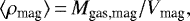
The disk material at Rmag is forced to move along the B-lines (because the magnetic pressure is equal to the ram pressure) filling the magnetosphere with a specific gas distribution. The density in this region allows us to calculate Tsub, and with a comparison with the dust temperature Tdust we can decipher whether or not there is dust in the magnetosphere, as this information is required to explain the light curve of V715 Per. To this end, we use the following simple estimate. The use of ρmag from Eq. (2) is included in the full modeling. The gas density in this region ρmag depends on Ṁ and the time it takes to arrive at the stellar surface starting its journey at Rmag. The mean of ρmag is calculated as
 (6)
(6)
where  is the volume of the magnetosphere and Mgas,mag is the gaseous mass inside the magnetosphere, estimated with
 (7)
(7)
where tff = Rmag∕vff with the free-fall velocity given by
 (8)
(8)
Making the required substitution in the previous equations, we find that ⟨ρmag⟩ = 2.93(5.29) × 10−15 g cm−3 and Tsub = 1019(1038) K for M⋆ = 0.906(0.56) M⊙. The two values for Tsub correspond to the two values for M⋆ (see Table 1). It is important to note that both values for Tsub are similar, such that the uncertainty in M⋆ is not relevant for the results presented here. Assuming a more realistic estimate for ⟨ρmag⟩, considering that the material is restricted inside an axisymmetric stream limited by magnetic field lines in the dipolar configuration (r ∝ sin2θ), we estimate that only 12% of the magnetospheric volume is covered with material. Because Tsub is not highly dependent on ρ, the new estimate (Tsub = 1094(1106) K) is close to the previous one. The estimate of Tsub comes from a linear interpolation of Table 3 of Pollack et al. (1994). Assuming an optically thin environment with typical dust composition and grains size distribution (see Sect. 4.1), the estimated temperature in the magnetosphere is Tmag ~ 1309 K which is larger than Tsub. This temperature is at the outskirts of the magnetosphere. There is no dust in a region close to the magnetospheric spots, where the temperature is up to ~7000 K. Starting at some minimum radius, there is a shell of evaporating dust up to Rmag. In order to find the gas temperature inside the magnetosphere, Hartmann et al. (1994) assumed a volumetric heating rate ∝ R−3 coming from a flux of Alfven waves during the gas accretion, which is cooled with a given radiative cooling rate. We conclude from this estimate that the grains will evaporate inside the magnetosphere.
In a study of the formation and evolution of chondrules inside a protoplanetary disk, Shu et al. (1996) estimated that the sublimation timescale, tsub, is about a few hours when the grains are heated to above Tsub. Using the stellar parameters from Table 1, tff = 6.79(7.56 h (M⋆ = 0.906(0.56) M⊙). It is therefore reasonable to assume the existence of a dusty layer in the funnel flow because tsub ~ tff.
For an estimate of the width of this layer, we included in this work the evaporating process as described in Xu et al. (2018). The rate at which the grain size is reduced at the temperature Tdust is given by
 (9)
(9)
where J is the net sublimation mass-loss flux and ρdust is the density of the dust grains, respectively. The expression for J is given by
![Mathematical equation: \begin{equation*} J(T_{\textrm{dust}})\,{=}\,{\alpha_{\textrm{subl}}[P_{\textrm{sat}}-P_{\textrm{g}}]\over c_{\textrm{s}}\sqrt(2\pi)}, \end{equation*}](/articles/aa/full_html/2020/11/aa38594-20/aa38594-20-eq12.png) (10)
(10)
and comes from the kinetic theory of gases. Here, αsubl is the evaporation coefficient, Psat is the saturation pressure (where the condensation and sublimation are in equilibrium),  is the gas pressure, and finally cs is the sound speed. Besides Pg, there are the gas ram pressure and the magnetic pressure which are in equilibrium. For the modeling, αsubl = 0.1 and ρdust = 3g cm−3 are taken as typical values. The expression for Psat is written as
 (11)
(11)
with A = 65 000 K and B = 35 for a generic refractory material (Xu et al. 2018). For the analysis presented in this work, A, B, ρdust, and αsubl are fixed but the specific characteristics of the system that we do not know a priori will lead to changes in these values. The evaporation process occurs when Psat > Pg and condensation occurs when Psat < Pg. For example, at Tdust = 1500 K (typical value for dust sublimation), the value of Psat leads to condensation instead of sublimation. For Tdust = 2000 K, Psat increases byfive orders of magnitude, such that the evaporation stage is reached. For Tdust = 7000 K, Psat increases bya further 10 orders of magnitude such that the dust only survives in a layer close to Rmag where Tdust is close to 1500 K.
As mentioned in Sect. 4.1, the grains are distributed according to a power-law; in the Appendix A we show that during the evaporation process the power of the size distribution is conserved. Also in Appendix A, we explain how the opacity at each point in a stationary stream is calculated, which includes the fact that the evaporation decreases the dust abundance.
Because the power-law shape of the size distribution is conserved, the survival of dust can be analyzed with the survival of the grains in the magnetosphere with the largest size smax using Eq. (9). We describe this process using a two-step algorithm, of which the steps are as follows: (1) For each point in the magnetosphere we identify whether or not it is located over a B-line that belongs to the stream limited by Rin and Rout (see Sect. 3.1). (2) We check whether or not there is dust. The condition is: if smax ≥ 0.25 μm then there is dust at this point; see Appendix A for details. The grains with sizes smaller than s = 0.25 μm will quickly disappear in the harsh environment to which the particles are exposed from there on, following their trajectory towards the stellar surface. We use the ballistic velocity field of Hartmann et al. (1994), the shape of the B-line, and Eq. (9) to describe the evaporation process along the trajectory. In this equation, we substitute ρmag from Eq. (2).
Repeating the two-step dust-survival algorithm for every point in the region surrounding Rmag leads to a dust distribution that depends on R, θ, and ϕ. However, in order to estimate the typical radial width of the dusty layer, we apply the algorithm along different LOSs in order to sample the complete region and decipher how far into the stream the optically thin dust can survive. This latter distance depends on the temperature of the stream (Tthin) which for a given dust composition, grain size distribution, and for a fixed stellar luminosity only depends on the distance to the star. For V715 Per at R = 0.4 Rmag, Tthin = 2221 K which corresponds to Psat ≫ Pg. At this state, a grain of s = 1 mm sublimates in about 1hr which is a factor of seven lower than tff, which means that grains rapidly disappear at this location and dust closer to this radius is not present. At the outskirts of the stream at R = Rmag, Tthin = 1479 K, Psat < Pg, and the process is condensation instead of sublimation. This clearly means that the dust particles being incorporated into the stream survive and steadily decrease in size until they are completely evaporated as they move in the stream towards the star. Between R = 0.7 and R = 0.8 Rmag, Psat = Pg and the condensation turns into sublimation. This means that the dusty radial width is larger than 0.2 Rmag, and therefore there is dust inside the magnetosphere that can shape the optical light curve. This estimate is done using a distribution of grains with smax = 1 mm. In Sect. 6, we show that according to the maximum grain size at the base of the stream, the radial width of the dusty layer varies.
We note that when the gas transits from the disk to the stream, there is probably a selection process in terms of the size of the grains that can make the journey. This is because the first grains that are incorporated into the stream are the ones located in the disk atmosphere where their size distribution is assumed to be consistent with the dust in the ISM (this is because detailed disk models,such as in D’Alessio et al. 2006, show grain settling towards the midplane). As we do not know the details of this process, a reasonableassumption is to consider that grain size at the base of the stream is distributed according to a power-law with given smax, which becomes the relevant free parameter to tune the modeling. Appendix A provides details of the survival of dust as the material moves towards the star.
5 Parameters for the modeling
5.1 Fixed parameters
From Grinin et al. (2018), we extract the stellar parameters (M⋆, R⋆,T⋆) noting that there are two values for M⋆: 0.56 M⊙ (LeBlanc et al. 2011) and 0.906 M⊙ (Kirk & Myers 2011). The distance to IC 348, where the source is located, is 315 pc. Using a mean of the estimates in Dahm (2008) we fix Ṁ = 5 × 10⁻⁹. The light curve period is P = 5.25 days (Grinin et al. 2018), which is a value very close to the rotational period of the star, namely Prot = 5.221 days (Cohen et al. 2004). The inclination of the system is assumed as i = 77°, as the largest value expected such that the outside part of the disk is not blocking the stellar radiation (Nagel & Bouvier 2019).
Variations in the size distribution of the dust grains change the opacity (κ), meaning that a consistent change in the stream dust-to-gas mass fraction (ζstream) is required to explain the observations. In other words, there is a degeneracy between these latter two variables. However, in the evaporation process that we include in the modeling, the grain size distribution is calculated at each point in the stream. The standard dust-to-gas mass fractions are fixed at typical values, ζsil = 0.004 and ζgrap = 0.0025 for the silicate and the graphite components, such that ζstd = ζsil + ζgrap = 0.0065. Using this, we fix κ. In the same process, ζstream is calculated because surface material continuously evaporates from each grain as the particles move from the base of the stream towards the star. This means that the spatial distribution of dust including the grain size distribution (a power law with a consistently calculated smax) is taken into account when using the algorithm for dust survival (see Sect. 4.2).
5.2 Free parameters
According to the modeling, the dust responsible for shaping the light curves is located in the magnetosphere. As ρmag is consistent with the observed Ṁ then in order to explain the depth of the section of the light curve interpreted as the stellar eclipse with the magnetospheric streams, we focus on one free parameter, namely the maximum grain size at the base of the stream smax,base.
As explained in Appendix A, the grain size distribution at the base of the stream is a power-law with an exponent of − 3.5 with a minimum grain size of smin = 0.005 μm, and the maximum grain size of smax,base is taken as the only free parameter. The range of this latter is between 0.25 μm, the value associated to the ISM (Mathis et al. 1977) and 1 mm, a value typical of the densest environment in a protoplanetary disk. We note that κ changes by more than an order of magnitude between the large grain distribution and the small grain distribution, and therefore it can be tuned through smax,base to explain the amplitude of the light curve. Using κ, the gas density (ρg), and ζstream we can check whether or not the dust is optically thin for each LOS. Including grain evaporation, the system state moves towards an optically thin scenario, the basic requirement to explain the observations.
6 Modeling
The three states of the light curve are: (1) a 5.25 d periodic signal of Δmag ~ 0.1, (2) a 5.25-d periodic signal that decreases in amplitude (Δmag < 0.1), and (3) very deep Algol-like minima reaching amplitudes of up to Δmag = 1 on a timescale of days. At any time during the observations, there is a periodic signal with evolving amplitude, and the Algol-like minima is superposed to the periodic signal. However, in the latter case, the dominant behavior is the one with the signal of greatest amplitude. As mentioned by Grinin et al. (2018), all states are interpreted by stellar extinction, such that the changes in the amount of dust surrounding the object should explain the observed variability. State (1) is the one we explain in detail in Sect. 6.1, where we use dust distributed along the B-lines consistent with the value used for Ṁ, such that we name it the low-Ṁ state. State (2) is interpreted by Grinin et al. (2018) based on the assumption that a larger Ṁ reduces Rmag such that the blocking structure decreases its area resulting in a decrease of Δmag. The variability of Ṁ is suggested by the measurements of EW(Hα) at different times by Herbig (1998), Luhman et al. (1998), and Dahm (2008). The first two measurements of EW(Hα), by Herbig (1998) and Luhman et al. (1998), were taken outside the epoch of enhanced activity represented in the observations by Dahm (2008), and therefore both regimes were sampled. Our interpretation differs from what has previously been stated, namely that a larger Ṁ (leading to a more powerful accretion shock) means a decrease in the amount of dust occulting the star because the stellar heating increases. A state with a larger Ṁ is expected in Classical T Tauri stars caused by their intrinsic variability. The Algol-like minimum identifying state (3) is simply an UX Ori-like event (stochastic fluctuations of the circumstellar extinction) where continuously accumulating material is explosively released to the star. The duration of the Algol-like minimum is about a week, meaning that the delivery of an unusual amount of gas (and dust) occurs continuously during (1–2) stellar rotations.
6.1 The low-Ṁ state: fiducial models
The value for Ṁ for V715 Per is estimated by Dahm (2008) using different optical and infrared lines. We name the models presented in this section the “fiducial models” because we include the stellar heating as the only source of heating.
The entire interpretation of the results is based on two competing mechanisms. The first one is that when Psat < Pg in all the cells of the system, the system is in the nonevaporating stage. On the other hand, when Psat > Pg, the system is in the evaporating stage. We note that an increment in smax,base leads to a decrease in Tdust, and with this Psat decreases, eventually making the system prone to condensation instead of sublimation, resulting in a large optical depth. Decreasing smax,base from its maximum value, the system changes from the nonevaporating stage to the evaporating stage. The latter stage is mixed with the other mechanism: an increment in the grain size leads to a decrease in κ, resulting in a decrement of the optical depth (τ). Thus, in theevaporating stage, the evaporation in itself reduces the opacity because a certain amount of dust disappears; on the other hand the evaporation reduces the grain size and the opacity increases.
The light curves depend on the gas-density distribution and the opacity of the dust located in the gaseous structures. Therefore, we present color maps of ρg and κ for an azimuthal cut at different phases showing the case with smax,base = 1 mm in Figs. 1 and 2. In Fig. 1, it is clear that the gas follows a stream along the magnetic lines in the dipolar configuration. We note that at different phases, the shape of the stream is different and the modulation by Bpol (see Eq. (2)) stands out in the plot corresponding to phase = 0.5. In Fig. 2, the low values of κ are associated to the large value for smax,base. A small amount of evaporation is present at the tip of the stream.
The spatial distribution of dust (characterized by ζstream and smax) is given using the evaporation algorithm, (see details in Appendix A) which is used to find smax,base consistent with Δmag = 0.1. The parameters used in the evaporation model imply that the dust can survive close to the star, as can be seen in Fig. 2.
For smax,base = 1 mm, Δmag ~ 0.00724, which is more than an order of magnitude lower than the value extracted from the observed light curves. For smax,base = 1 μm, Δmag ~ 0.00917, which is also less than expected. We note that these two models, while representing two extreme cases, produce similar small values for Δmag. This can be explained by the fact that for smax,base = 1 μm, ζstream decreases because of strong evaporation, and for smax,base = 1 mm, evaporation is not important, but the opacity of large grains is small. For this reason, we argue that there is a value of smax,base in between the previous values that is able to explain the observed Δmag. As shown in the modeled light curves presented in Fig. 3, either smax,base = 10 or 100 μm are able to fit the requirement. In order to follow the trend in the light curves in Fig. 3, we present the models for smax,base = 1, 10, 100 μm, and 1 mm. The trend shown in Fig. 3 is not monotonous, that is, Δmag does not increase or decrease when smax,base increases. We discuss the various modeled light curves below.
The shape of the light curves for smax,base = 1000 μm (model A) and 100 μm (model B) are similar. The model B has larger Δmag than model A which means that τ100 > τ1000. Because the mean grain size ⟨s⟩ is smaller in model B, the opacity κ100 is larger (τ100 is larger) compared to the value in model A, such that this effect dominates over the decrement of κ100 due to the evaporation process.
The shape of the light curves corresponding to smax,base = 100 μm (model B) and 10 μm (model C) mainly differ because the maximum in Δmag shifts from the phase = 0.5 to phase = 0.3. Model B is in the nonevaporating stage and Model C is in the evaporating stage because Psat ≫ Pg. The behavior of Model B is completely determined by nonevaporation, but in model C the evaporation reduces ζstream which compensates the increment of κ due to the decrement of ⟨s⟩, resulting in Δmag100 ~ Δmag10.
The shapes of the light curves for smax,base = 10 μm (model C) and 1 μm (model D) are similar. However, Δmag1 ≪ Δmag10, which means that the strong evaporation increasing from model C to model D leads to a dominant ζstream decrement over the κ increment associated to a decrement in ⟨s⟩.
The light curves of models B and C are different (see Fig. 3). The main difference is that the maximum of Δmag changes from phase = 0.5 (the azimuthal configuration where the maximum in density is located) in model B to phase = 0.3 in model C. In order to explain how the shape of the light curves changes for different smax,base, we present color maps for these two phases. Figures 4 and 5 show κ color maps for different values of smax,base at phase = 0.3 and phase = 0.5, respectively. We note that in model C, ⟨s⟩ decreases slower in a denser region because ṡ ∝ Psat − Pg, but at the same time τ decreases faster due to the amount of material evaporated. In addition, smax,base decreases from model B to C, increasing κ. The result is that in model C at phase = 0.5 (largest density), the evaporation dominates over the other mechanisms, increasing τ, and at phase = 0.3, the increment of κ due to a smaller smax,base dominates over evaporation in a lower density region. This results in a shift of Δmag maximum between models B and C.
We note that, in the framework of this model, regardless of the manner in which the dust is distributed, the only way to explain Δmag = 0.1 is with an optically thin scenario. Our best model leads to a mean optical depth ⟨τ⟩ around ⟨τ⟩ = 0.092, which is the required value to explain the observed Δmag.
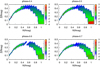 |
Fig. 1 Density for different phases. This is part of the data used to find the light curves in Fig. 3. Here, we show the model with smax,base = 1 mm. |
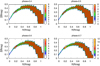 |
Fig. 2 Opacity for different phases. This is part of the data used to find the light curves in Fig. 3. Here, we show the model with smax,base = 1 mm. |
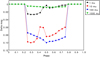 |
Fig. 3 Light curve for V715 Per consistent with Ṁ = 5 × 10⁻⁹ M⊙ yr−1; smax,base = 1 μm (black line), smax,base = 10 μm (red line), smax,base = 100 μm (blue line), smax,base = 1 mm (green line). |
6.2 The low-Ṁ state: higher temperature models
We name the models presented in this section the “high-temperature models” because we assume that the temperature can increasedue to heating caused by the deposition of heat by Alfven waves as mentioned in Hartmann et al. (1994). As explained in Sect. 4.2, the dust cannot survive at the high temperatures (up to ~ 7000 K) present in most of the region limited by Rmag. In order to analyze the effect of increasing the temperature, we show the opacity distribution for the cases smax,base = 1, 10, 100 μm, and 1 mm when fixing Tdust to 2000 K. The color maps are shown in Figs. 6 and 7. There is clearly more evaporation in all of the high-temperature models than in the fiducial models. In Fig. 7, we can see that the high-temperature model with smax,base = 1 mm shows an increase in opacity compared with the fiducial model. In other words, Psat increases such that Psat > Pg, in this way reaching the evaporation stage. At this stage, the grain size decreases and the opacity increases. Because of the high inclination, the dust occulting the star is located close to Rmag where the opacity is the lowest, leading to a low-amplitude light curve, which is not able to explain the observed light curve. For the other models, the opacity decreases, such that these models are not able to explain the observed light curve. Our conclusion is that the surviving dust is restricted to a thin layer where the precise width depends on a detailed modeling of the stream heating by Alfven waves.
We note that the high-temperature model with smax,base = 1 mm in Fig. 7 clearly shows that as the material moves towards the star, the opacity increases due to the decrease in smax, but finally thereis an opacity decrease because the amount of material evaporated dominates over the decrement in smax.
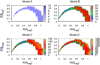 |
Fig. 4 Opacity for the phase = 0.3. This is part of the data used to find the light curves in Fig. 3. Here, we show model A (smax,base = 1 mm, upper left plot), model B (smax,base = 100 μm, upper right plot), model C (smax,base = 10 μm, lower left plot), and model D (smax,base = 1 μm, lower right plot). |
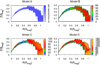 |
Fig. 5 Opacity for the phase = 0.5. This is part of the data used to find the light curves in Fig. 3. Here, we show model A (smax,base = 1 mm, upper left plot), model B (smax,base = 100 μm, upper right plot), model C (smax,base = 10 μm, lower left plot), and model D (smax,base = 1 μm, lower right plot). |
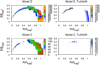 |
Fig. 6 Opacity for the phase = 0.5. Here, we show the fiducial models: smax,base = 1 μm (upper left plot), and smax,base = 10 μm (lower left plot) complemented with the high temperature models: smax,base = 1 μm, Tdust = 2000 K (upper right plot), and smax,base = 10 μm, Tdust = 2000 K (lower right plot). |
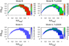 |
Fig. 7 Opacity for the phase = 0.5. Here, we show the fiducial models: smax,base = 100 μm (upper left plot), and smax,base = 1 mm (lower left plot) complemented with the high temperature models: smax,base = 100 μm, Tdust = 2000 K (upper right plot), and smax,base = 1 mm, Tdust = 2000 K (lower right plot). |
7 Conclusions
The main conclusions of our analysis and modeling of the dipper light curve of V715 Per can be summarized as follows:
- (1)
The dust can survive at Rmag where the disk is truncated for reasonable parameters of the density of the optically thick disk;
- (2)
Assuming that the gas is distributed following the stellar B-lines, using the values for the observed Ṁ, and a standard dust-to-gas ratio without evaporation, the dust in the magnetosphere is optically thick (⟨τ⟩ = 2.76). Our best model with evaporation included is able to explain the observations. The value for ⟨τ⟩ associated to the model is close to the required value
 in the optically thin regime;
 - (3)
The low gas density and the radial range of the magnetosphere mean that in most of the atmosphere Tdust > Tsub, and therefore the dust cannot survive. Nevertheless, the dust is able to survive in a shell with an outer radius given by Rmag, because the timescales for evaporation (tsub) and free-fall towards the stellar surface (tff) are similar;
- (4)
We find a model using the largest size of the grains at the base of the magnetospheric stream, smax,base, as a free parameter. We find that the models with smax,base = 10, 100 μm are able to explain the observed amplitude of the optical light curve (Δmag). The grains move towards the star and evaporate, changing their size and shaping the light curve;
- (5)
The analysis of the models presented in Sect. 6.1 suggests that two competing mechanisms are simultaneously responsible for the shape of the light curves. The first is evaporation, which reduces the dust density leading to a decrement of the dip amplitude. However, during this process, the mean size of the grain decreases and the dip amplitude increases because the grain opacity increases. As smax,base changes, the contribution of both mechanisms also changes, and therefore the depth and shape of the light curves vary accordingly;
- (6)
In the modeling, we do not include the deposition of heat by Alfven waves in the stream as suggested by Hartmann et al. (1994), which would considerably increase the temperature inside the magnetosphere. At such a high temperature (~ 7000 K), the grains evaporate almost instantly, thereby restricting the dust to a thin layer very close to Rmag. In any case, due to the high inclination of the system, almost all the blocking structure is close to Rmag, a fact that can be verified in any of the color maps where the shape of the stream can be seen;
- (7)
Because the values for M⋆ (the main parameter used to calculate tff) and Ṁ (the main parameter used to calculate Rmag) for V715 Per are typical of many other systems showing this behavior in their light curves, this mechanism can be invoked to explain the light curves where the flux shows color changes associated with circumstellar extinction, which indicates that the occulting dust is optically thin.
The most important result of this work is that the dust inside the magnetosphere is relevant to explain light curves and should be taken into account for a full interpretation of the system. Analysis of a large set of objects should reveal features showing the complexity of YSOs.
Acknowledgements
This project has received funding from the European Research Council (ERC) under the European Union’s Horizon 2020 research and innovation program (grant agreement No 742095 ; SPIDI : Star-Planets-Inner Disk- Interactions; http://www.spidi-eu.org). E.N. appreciate the support at the Institut de Planétologie & d’Astrophysique de Grenoble (IPAG) by Observatoire des Sciences de l’Univers de Grenoble/Université Grenoble Alpes (OSUG/UGA) while in a sabbatical stay where part of this work was done.
Appendix A Abundance, opacity, and grain-size distribution of the dust in the evaporating magnetospheric stream.
As the grains in the magnetospheric stream move towards the star, Psat surpasses Pgas and the dust starts to evaporate. This process is not instantaneous; the grain decreases its size at a rate given by ṡ as described in Sect. 4.2. During this process, all the grains decrease in size. In the following we show that the power-law grain size distribution is conserved.
The number of grains within the size range [s, s + ds] is: Cs−3.5ds, with C being a normalization coefficient. The number of grains is conserved after the span of time dt if d s changes to ṡ d t + ds. The size distribution,f(s, t), satisfies the equation
 (A.1)
(A.1)
which can be written as
 (A.2)
(A.2)
where g is a constant. From the total differential we can identify the terms  and
and  and using the fact that
  , we find that
 (A.3)
(A.3)
The above equation can be solved using the initial condition f(s, t = 0) = Cs−3.5 such that f(s, t) = Cs′−3.5, where s′ = s −ṡt is the size of the grain after time t. We note that the power law is conserved with the same exponent.
In a stationary configuration, each location of the stream has an assigned value for smax. In the ISM and in the disk, the typical size distributions are characterized by smin = 0.005 μm; for simplicity we keep this value here. For the estimate of smax we use ṡ which requires the radial velocity given in Hartmann et al. (1994) calculated for ballistic infall from rest at Rmag used to calculate the density, such that smax decreases as the dust moves closer to the star.
The dust opacity at each point is calculated as a time-dependent process starting with the opacity of the distribution of large grains (smax = smax,base) associated with the dust in the disk, finally arriving at the case where smax ≥ 0.25 μm. Here, smax = 0.25 μm is the value associated with the distribution of small grains, which is typical of the ISM, the lowest value considered here. A grain with smax < 0.25 μm completely evaporates over a short time-span compared to the time it takes to arrive at this point. Therefore, we assume that there is dust in a streamline if smax ≥ 0.25 μm.
The opacity associated with the dust distributed with 0.25μm < smax < 1 mm is calculated by interpolating between the opacity of the large grains and the distribution of small grains of the standard abundance, ζstd = 0.0065.
We correct the opacity by including the fact that the dust abundance decreases as each grain decreases in radius during the gradual evaporation of its superficial mass. This process should be included starting from the base of the stream. The correction factor is calculated using the total initial dust mass (Minit) in a volume ΔV and the mass evaporated Mevap over a time-span Δt.
From the initial dust abundance ζinit, Minit = ζinitρgΔV, where ρg is the gas density. On the other hand, we can write
 (A.4)
(A.4)
Equating both expressions,
![Mathematical equation: \begin{equation*} C\,{=}\,{3\zeta_{\textrm{init}}\rho_{\textrm{g}}\Delta V\over 8\pi\rho_{\textrm{dust}}[s_{\textrm{max}}^{0.5}-s_{\textrm{min}}^{0.5}]}. \end{equation*}](/articles/aa/full_html/2020/11/aa38594-20/aa38594-20-eq26.png) (A.5)
(A.5)
After the integration time Δt, the evaporated dust mass is
 (A.6)
(A.6)
The corrected dust abundance ζ is calculated using
 (A.7)
(A.7)
and performing all the straightforward integrations.
Now, for the next integration time smax = smax −ṡΔt and ζinit = ζ and this algorithm is repeated until the requested stream point is reached.
References
- Alencar, S. H. P., Teixeira, P. S., Guimaraes, M. M., et al. 2010, A&A, 519, A88 [NASA ADS] [CrossRef] [EDP Sciences] [Google Scholar]
- Baraffe, I., Chabrier, G., Allard, F., & Hauschildt, P. H. 1998, A&A, 337, 403 [Google Scholar]
- Barsunova, O. Yu., Grinin, V. P., & Sergeev, S. G. 2013, Astrophysics, 56, 395 [CrossRef] [Google Scholar]
- Barsunova, O. Yu., Grinin, V. P., Sergeev, S. G., Semenov, A. O., & Shugarov, S. Yu. 2013, Astrophysics, 58, 193 [CrossRef] [Google Scholar]
- Barsunova, O. Yu., Grinin, V. P., Arharov, A. A., et al. 2016, Astrophysics, 59, 147 [CrossRef] [Google Scholar]
- Bouvier, J., Chelli, A., Allain, S., et al. 1999, A&A, 349, 619 [NASA ADS] [Google Scholar]
- Cody, A. M., Stauffer, J., Baglin, A., et al. 2014, AJ, 147, 82 [NASA ADS] [CrossRef] [Google Scholar]
- Cohen, R. E., Herbst, W., & Williams, E. C. 2004, AJ, 127, 1602 [NASA ADS] [CrossRef] [Google Scholar]
- Dahm, S. E. 2008, AJ, 136, 521 [NASA ADS] [CrossRef] [Google Scholar]
- D’Alessio, P., Hartmann, L., Calvet, N., et al. 2005, ApJ, 621, 461 [NASA ADS] [CrossRef] [MathSciNet] [Google Scholar]
- D’Alessio, P., Calvet, N., Hartmann, L., Franco-Hernández, R., & Servin, H. 2006, ApJ, 638, 314 [NASA ADS] [CrossRef] [Google Scholar]
- D’Antona, F., & Mazzitelli, I. 1997, Mem. Soc. Astron. It., 68, 807 [Google Scholar]
- Dodin, A. V., & Lamzin, S. A. 2012, Astron. Lett., 38, 649 [NASA ADS] [CrossRef] [Google Scholar]
- Flaherty, K. M., Muzerolle, J., Rieke, G., et al. 2013, AJ, 145, 66 [NASA ADS] [CrossRef] [Google Scholar]
- Fonseca, N. N.J., Alencar, S. H. P., Bouvier, J., Favata, F., & Flaccomio, E. 2014, A&A, 567, A39 [NASA ADS] [CrossRef] [EDP Sciences] [Google Scholar]
- Gregory, S. G., Jardine, M., Gray, C. G., & Donati, J. F. 2010, Rep. Progr. Phys., 73, 6901 [NASA ADS] [CrossRef] [Google Scholar]
- Grinin, V. P., Barsunova, O. Yu, Sergeev, S. G., Sotnikova, N. Ya, & Demidova, T. V. 2006, Astron. Lett., 32, 827 [NASA ADS] [CrossRef] [Google Scholar]
- Grinin, V. P., Stempels, H. C., Gahm, G. F., et al. 2008, A&A, 489, 1233 [NASA ADS] [CrossRef] [EDP Sciences] [Google Scholar]
- Grinin, V. P., Barsunova, O. Yu., Sergeev, S. G., et al. 2018, Astron. Rep., 62, 677 [CrossRef] [Google Scholar]
- Hartmann, L., Hewett, R., & Calvet, N. 1994, ApJ, 426, 669 [NASA ADS] [CrossRef] [Google Scholar]
- Herbig, G. H. 1998, ApJ, 497, 736 [NASA ADS] [CrossRef] [Google Scholar]
- Kirk, H., & Myers, P. C. 2011, ApJ, 727, 64 [NASA ADS] [CrossRef] [Google Scholar]
- Konigl, A. 1991, ApJ, 370, L39 [NASA ADS] [CrossRef] [Google Scholar]
- LeBlanc, T. S., Covey, K. R., & Stassun, K. G. 2011, AJ, 142, 55 [CrossRef] [Google Scholar]
- Luhman, K. L., Rieke, G. H., Lada, C. J., & Lada, E. A. 1998, AJ, 508, 347 [NASA ADS] [CrossRef] [Google Scholar]
- Luhman, K.L., Stauffer, J. R., Muench, A. A., et al. 2003, ApJ, 593, 1093 [NASA ADS] [CrossRef] [Google Scholar]
- Lynden-Bell, D., & Pringle, J. E. 1974, MNRAS, 168, 603 [NASA ADS] [CrossRef] [Google Scholar]
- Mathis, J. S., Rumpl, W., & Nordsieck, K. H. 1977, ApJ, 217, 425 [NASA ADS] [CrossRef] [Google Scholar]
- McGinnis, P. T., Alencar, S. H. P., Guimaraes, M. M., et al. 2015, A&A, 577, A11 [NASA ADS] [CrossRef] [EDP Sciences] [Google Scholar]
- Morales-Calderón, M., Stauffer, J. R., Hillenbrand, L. A., et al. 2011, ApJ, 733, 50 [NASA ADS] [CrossRef] [Google Scholar]
- Nagel, E., & Bouvier, J. 2019, A&A, 625, A45 [CrossRef] [EDP Sciences] [Google Scholar]
- Nagel, E., D’Alessio, P., Calvet, N., et al. 2010, ApJ, 708, 38 [NASA ADS] [CrossRef] [Google Scholar]
- Pollack, J. B., Hollenbach, D., Beckwith, S., et al. 1994, ApJ, 421, 615 [NASA ADS] [CrossRef] [Google Scholar]
- Romanova, M. M., Ustyugova, G. V., Koldova, A. V., et al. 2013, MNRAS, 430, 699 [NASA ADS] [CrossRef] [Google Scholar]
- Ruiz-Rodriguez, D., Cieza, L. A., Williams, J. P., et al. 2018, MNRAS, 478, 3674 [NASA ADS] [CrossRef] [Google Scholar]
- Sicilia-Aguilar, A., Manara, C. F., de Boer, J., et al. 2020, A&A, 633, A37 [CrossRef] [EDP Sciences] [Google Scholar]
- Shu, F. H., Shang, H., & Lee, T. 1996, Science, 271, 1545 [NASA ADS] [CrossRef] [Google Scholar]
- Stauffer, J., Cody, A. M., McGinnis, P., et al. 2015, AJ, 149, 130 [Google Scholar]
- Stauffer, J., Cody, A. M., Rebull, L., et al. 2016, AJ, 151, 60 [NASA ADS] [CrossRef] [Google Scholar]
- Xu, S., Rappaport, S., van Lieshout, R., et al. 2018, MNRAS, 474, 4795 [CrossRef] [Google Scholar]
All Tables
All Figures
|
Fig. 1 Density for different phases. This is part of the data used to find the light curves in Fig. 3. Here, we show the model with smax,base = 1 mm. |
| In the text | |
|
Fig. 2 Opacity for different phases. This is part of the data used to find the light curves in Fig. 3. Here, we show the model with smax,base = 1 mm. |
| In the text | |
|
Fig. 3 Light curve for V715 Per consistent with Ṁ = 5 × 10⁻⁹ M⊙ yr−1; smax,base = 1 μm (black line), smax,base = 10 μm (red line), smax,base = 100 μm (blue line), smax,base = 1 mm (green line). |
| In the text | |
|
Fig. 4 Opacity for the phase = 0.3. This is part of the data used to find the light curves in Fig. 3. Here, we show model A (smax,base = 1 mm, upper left plot), model B (smax,base = 100 μm, upper right plot), model C (smax,base = 10 μm, lower left plot), and model D (smax,base = 1 μm, lower right plot). |
| In the text | |
|
Fig. 5 Opacity for the phase = 0.5. This is part of the data used to find the light curves in Fig. 3. Here, we show model A (smax,base = 1 mm, upper left plot), model B (smax,base = 100 μm, upper right plot), model C (smax,base = 10 μm, lower left plot), and model D (smax,base = 1 μm, lower right plot). |
| In the text | |
|
Fig. 6 Opacity for the phase = 0.5. Here, we show the fiducial models: smax,base = 1 μm (upper left plot), and smax,base = 10 μm (lower left plot) complemented with the high temperature models: smax,base = 1 μm, Tdust = 2000 K (upper right plot), and smax,base = 10 μm, Tdust = 2000 K (lower right plot). |
| In the text | |
|
Fig. 7 Opacity for the phase = 0.5. Here, we show the fiducial models: smax,base = 100 μm (upper left plot), and smax,base = 1 mm (lower left plot) complemented with the high temperature models: smax,base = 100 μm, Tdust = 2000 K (upper right plot), and smax,base = 1 mm, Tdust = 2000 K (lower right plot). |
| In the text | |
Current usage metrics show cumulative count of Article Views (full-text article views including HTML views, PDF and ePub downloads, according to the available data) and Abstracts Views on Vision4Press platform.
Data correspond to usage on the plateform after 2015. The current usage metrics is available 48-96 hours after online publication and is updated daily on week days.
Initial download of the metrics may take a while.