| Issue |
A&A
Volume 696, April 2025
|
|
|---|---|---|
| Article Number | A46 | |
| Number of page(s) | 5 | |
| Section | Interstellar and circumstellar matter | |
| DOI | https://doi.org/10.1051/0004-6361/202453365 | |
| Published online | 01 April 2025 | |
A dusty magnetospheric stream as the physical mechanism responsible for stellar occultations: Interpretation of the TESS light curve of the pre-transitional disk system UX Tau A
1
Departamento de Astronomía, Universidad de Guanajuato, Callejón de Jalisco, S/N,
36240
Guanajuato,
Mexico
2
Univ. Grenoble Alpes, CNRS, IPAG,
38000
Grenoble,
France
★ Corresponding author; This email address is being protected from spambots. You need JavaScript enabled to view it.
Received:
9
December
2024
Accepted:
21
February
2025
Abstract
Context. Recent observations of the object UX Tau A containing a pre-transitional disk suggest that the inner disk is misaligned and precessing with respect to the outer disk. These motions lead to a highly dynamic environment that changes the reservoir of dust feeding the star. One of the effects of this is seen in the features of the Transiting Exoplanet Survey Satellite (TESS) optical light curve (LC), resembling dips of variable depth changing within the timescale of the inner disk dust replenishment.
Aims. For this work we interpreted the TESS LC corresponding to a time window around the date a spectrum was taken with the James Webb Space Telescope (JWST). The spectrum was taken in the mid-infrared, clearly a range tracing the emission of dust. Compared with previous spectra, the most recent spectrum suggests a strong decrease in the amount of dust in the inner disk; the observed spectral energy distribution shows a very small infrared excess.
Methods. The physical modeled flux comes from stellar radiation occulted by a sheet of evaporating dust following the magnetospheric field (B⋆) lines. A grid of stream configurations were taken where the gas component explains the JWST spectrum and the Hα profiles.
Results. Our quest to find a reasonable interpretation of the LC requires a tuning of the values associated with the truncation radius, the inclination of the disk with respect to the line of sight and the maximum size of the dusty grains.
Conclusions. We conclude that the dust evaporation accretion flow is able to explain the typical depths of the LC features periodically changing with the stellar rotational period. We conclude that the dust evaporation accretion flow is able to explain the dips observed in the UX Tau A TESS light curve, most notably the large amplitude dips up to Δmag ∼ 0.7 mag, while the lower level variability events (Δmag ≤ 0.2 mag) in the LC could also be accounted for by the periodic modulation caused by a hot surface spot. We also suggest that winds and warps are unlikely mechanisms for UX Tau A’s variability.
Key words: circumstellar matter / stars: pre-main sequence
© The Authors 2025
 Open Access article, published by EDP Sciences, under the terms of the Creative Commons Attribution License (https://creativecommons.org/licenses/by/4.0), which permits unrestricted use, distribution, and reproduction in any medium, provided the original work is properly cited.
This article is published in open access under the Subscribe to Open model. This email address is being protected from spambots. You need JavaScript enabled to view it. to support open access publication.
1 Introduction
The variability observed in T Tauri stars leads us to realize that time-dependent physical mechanisms occurring in different regions of the system shape the emission at different wavelengths. Observations in the radio wavelength range refer to processes in the cold outer parts of the disk (Doi 2024; Ribas et al. 2024; Pinilla et al. 2024). In the inner disk, the heated dust mainly emits in the infrared (IR), such that variations in the spectra can be attributed to structural changes in the system shaped by the interaction of the stellar magnetic field with the disk (McGinnis et al. 2015; Bouvier et al. 1999; Alencar et al. 2018) or within the disk (Morales-Calderón et al. 2011; Espaillat et al. 2011; Flaherty et al. 2012). Inhomogeneities in the inner disk that formed in the unstable regime of accretion are also processes characterizing the inner disk structure where the IR flux is produced (Ingleby et al. 2015). The optical flux comes from the star and the variations in this flux are due either to changes on the stellar surface, mainly associated with time-dependent modifications of the location and shape of cold and hot spots (Kulkarni & Romanova 2013), or to the dynamics of dusty structures surrounding the star (Nagel & Bouvier 2023).
The driving idea for this work comes from the analysis of new evidence of the object UX Tau A by Espaillat et al. (2024). A spectrum taken with the James Webb Space Telescope (JWST) suggests that at the observing date the emission of dust surrounding the star is very low; the authors argue that dust is depleted in the inner disk of the pre-transitional disk (Pre-TD). They compare this spectrum with others taken over the years to justify that the amount of dust changes according to a replenishment timescale of around 0.1 yr. This is possible if the inner and outer disk are misaligned (Bohn et al. 2022). As a result of this, we expect that during the span of time of the Transiting Exoplanet Survey Satellite (TESS) light curve (LC) (taken around the date when the JWST spectrum was taken, Espaillat et al. 2024), the amount of dust changes on a day-scale basis. Motivated by this, we present in this work a set of models estimating the dust occultation by evaporating grains moving along the B⋆ lines, as in Nagel & Bouvier (2020) and Nagel et al. (2024).Any physical model placing dust in the innermost regions of the disk, above the midplane at the required heights depends on the interaction of the magnetosphere with the disk.
Espaillat et al. (2024) argue that the inner disk is misaligned with respect to the outer disk and precessing, continuously changing the configuration of the two disks, which results in a time-dependent rate of feeding of dust from the outer to the inner disk. This scenario allows us to consider an abundance of dust at the base of the accretion stream in the midplane as a free-parameter in the modeling. Espaillat et al. (2024) also present a grid of models for UX Tau A consistent with the observations of the Hα profiles of four spectra using the magnetospheric accretion flow model from Hartmann et al. (1994). The Hα profiles are formed in the heated dust-free magnetospheric streams, as modeled by Espaillat et al. (2024), with dust located in the colder streamlines close to the disk midplane. From this fit, the intermediate values of the disk inclination (i) with respect to the line of sight (20 < i < 60∘) means that in order to explain the dipper behavior observed in its LC, a mechanism is required to move dust to higher altitudes. A known physical mechanism able to do this is called a propeller regime. Romanova et al. (2018) studied the accretion of material from the disk to the stellar surface via the magnetosphere, and concluded that if the magnetosphere rotates much more rapidly than the inner disk, then some of the material in the disk forms a wind; such a system is called a strong propeller. If the magnetosphere rotates slightly faster than the inner disk and the material accretes toward the star without a wind, such a system is called a weak propeller, where the magnetospheric radius (Rmag) is larger than the corotational radius (Rco). In the former, all the accreting material is channeled to a wind; in the latter, the material is distributed between a wind and magnetospheric accretion. If neither of the two conditions is fulfilled, then all the material accretes toward the star in magnetospheric streams. For example, the interpretation of the burster RU Lup using new evidence, allows Wojtczak et al. (2024) to argue the presence of a wind produced in the magnetospheric boundary consistent with a weak propeller regime of accretion. In the same frame, GRAVITY Collaboration (2023) suggest that CI Tau is in the regime of unstable accretion, placing the object in the burster category. Espaillat et al. (2024) also propose a scenario in Gaidos et al. (2024) where a magnetic disk wind (Blandford & Payne 1982) forms a dusty wall that blocks part of the stellar radiation. Liffman et al. (2020) uses the ejection of material at the inner disk edge as a source of variability in the infrared. In addition to the disk wind, another scenario to interpret LCs is the warp model used by Bouvier et al. (1999) to analyze AA Tau, the prototypical dipper; a model also used by McGinnis et al. (2015) to describe objects in NGC 2264 and by Sicilia-Aguilar et al. (2020) to interpret the LC of the young dipper RX J1604.3-2130A. The warp is caused by the interaction of the disk and the inclined stellar magnetic field, and is located at the boundary of these two components (Romanova et al. 2013). Its moderate scale-height restricts the modeling to dipper systems with i > 60∘.
Summarizing the previous ideas, we extract two relevant facts. The first is that UX Tau A is close to being, but is not in the weak propeller regime because Rco ≳ Rmag (Espaillat et al. 2024). The second is that the values of i estimated by the Hα modeling is in the range 20∘ < i < 60∘, values smaller than required in the warp model. We conclude that either the wind or the warp alone are not adequate scenarios to explain the TESS LC. In this work we decided to focus on the dusty magnetosphere model of Nagel & Bouvier (2020) and Nagel et al. (2024).
The analysis of the Hα profiles does not require the amount of dust in the stream; however, a consistent interpretation of the TESS LC depends on this value. Following the lead, we present in this work, the distribution of amplitudes of an optical LC (Δmag) coming from the occultation of the stellar radiation by evaporating grains inside the magnetosphere, taking as an input the stream configuration of the models fitting the Hα profiles.
The outline of the paper is as follows. In Sect. 2 we present the information required to explain the model used to interpret the TESS LC of UX Tau A. In Sect. 3 a grid of models is presented that identifies the effect of each parameter in a synthetic LC. In Sect. 4 several models consistent with the observations are presented with a discussion on the degeneracy of the models. Finally, our conclusions are presented in Sect. 5.
2 Model
The aim of the work is the interpretation of the TESS LC of UX Tau A observed during Sectors 70 and 71. The JWST Mid-Infrared Instrument (MIRI) spectrum of this object was taken during 2023 October 13, which coincides with Sector 70. Due to the nearly photospheric levels of this spectrum up to about 10 μm, Espaillat et al. (2024) argue that the amount of dust in the inner disk of the pre-transitional disk is small. Espaillat et al. (2024) use the Spitzer spectra taken between 2004 and 2008 to estimate a typical amount of dust in the inner disk, and with an estimate for Ṁ demonstrate that the amount of dust changes with time on a timescale of weeks. As a first step for the physical interpretation of the TESS LC, Espaillat et al. (2024) use the framework defined by Cody & Hillenbrand (2018) to categorize the type of LC as an aperiodic dipper. Aperiodic time series do not necessarily imply a chaotic LC, where periodic signals can be present. In this case, Espaillat et al. (2024) detects a periodic signal of 3.8d consistent with Sectors 43, 44, 70, and 71, corresponding either to a structure located around Rco = 6.38R⋆ (R⋆ is the stellar radius) or to the stellar rotational period estimated with the periodicity of a long-lived spot. We assume that the variability is associated with the first scenario. We took advantage of the modeling of the Hα profiles in Espaillat et al. (2024) to obtain a configuration for the magnetospheric streams that can be used as a “backbone” for the distribution of the dust responsible for producing the dips in the LC. The relevance of this modeling is that the degeneracy of models coming from the Hα profiles fit can be broken using the fit of the TESS LC presented in this work.
The free parameters used in the Hα fit are the inner disk radius equivalent to the truncation radius or to the size of the magnetosphere (Rmag), the width of the flow in the midplane (Wr), the maximum temperature in the stream (Tmax), and the mass accretion rate at the stellar surface (Ṁ) (see Thanathibodee et al. 2023, for details). A main parameter required to extract the emission is the gas temperature (Tg), which we assume in our modeling is equal to the dust temperature (Td). Espaillat et al. (2024) use Tg from the model by Hartmann et al. (1994), which was also used in Tessore et al. (2023) to model Brγ line emission in the magnetosphere of young stellar objects (YSOs). The model of Hartmann et al. (1994) is applicable inside dusty-free regions because at Tg > 5000 K the evaporation rate is fast (Xu et al. 2018). This means that the occulting dust comes from the colder regions close to the midplane where there is an enhanced cooling rate due to the higher density.
The evolution of dust is followed as in Nagel & Bouvier (2020), corresponding to grains evaporating as they move along the stream. We propose a scenario where the disk is truncated at locations where the dust can survive. The dust can exist inside and outside the magnetosphere. The boundary between these two regions is Rmag (Konigl 1989), a parameter related to stellar and disk parameters as in the fit using the 3D magnetic hydrodynamical (MHD) simulations by Takasao et al. (2022); this fit is
 (1)
(1)
where Ṁ−10 is Ṁ in units of 10−10 M⊙ yr−1, M⋆ is the stellar mass in units of solar mass, R⋆ is given in units of solar radius, and B⋆ is the intensity of the dipolar magnetic field at the equator.
In addition to the parameters defining the configuration of the streams, there are parameters associated with the dust, available to fit the amplitude of the LC. One of these parameters is the maximum size of the grains located in the stream (amax). The grain sizes are distributed in size according to a−3.5 as in the interstellar medium (Mathis et al. 1977). The upper threshold of amax is calculated as in Li et al. (2022) where this value corresponds to the largest grains dragged by the streams. Grains with larger sizes stay in the midplane as potential seeds to form larger objects, the first step for planet formation (Li et al. 2022). The upper threshold of amax depends on the gas density at the base of the stream, the grain density, and the disk height. The size of the grains should be below this value to actually represent grains that can be dragged into the stream.
Summarizing, the parameters fixed in the models presented in this work are M⋆, effective temperature of the stellar surface (T⋆), and R⋆. The free parameters are divided into two categories. The first contains Ṁ, Rmag, Wr, and i taken from the ranges associated with the Espaillat et al. (2024) models. The second category contains amax and dust abundance ζd, which are restricted to physical reasonable values. If not mentioned, we assume ζd = 0.01.
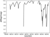 |
Fig. 1 Light curve from TESS during Sector 70 and the first part of Sector 71 as in Espaillat et al. (2024). The high-amplitude dips at JD 60 2240 and JD 60 2244 are clearly seen. |
3 Preliminary analysis
The aim of this work is the interpretation of the typical depths of the dips in the TESS LC of UX Tau A (Espaillat et al. 2024). During the 40-day span of the observations, we extracted three typical values in the TESS LC: Δmag∼(0.1, 0.2, 0.7) representing low-amplitude, middle-amplitude, and high-amplitude scenarios in the vicinity of the JWST spectrum date. We added the TESS LC in Fig. 1 as a reference to identify these features.
3.1 Grid of models
The first step we took to find an adequate interpretation of the LC was to define a grid of models. We used the fits for the Hα profiles in Espaillat et al. (2024) including the parameter uncertainties to define ranges for some of the variables required to obtain synthetic values for Δmag. The upper range of Rmag was extended from 5.7 to 6.4R⋆ to include the value of Rco. The range of Rmag also includes the range of sublimation radius (Rsub), as given in the analysis of dippers in Taurus by Roggero et al. (2021) using stellar heating. We assumed a range of sublimation temperature (Tsub) between 1500 and 2000 K, such that Rsub ranges between 3.8 and 6.8 R⋆.
Thus, the ranges coming from the Hα profile modeling are Ṁ = (1, 2, 3) × 10−8 M⊙ yr−1 (from now on we write Ṁ in units of M⊙ yr−1), i = (20, 30, 40, 44, 48, 52, 56, 60)∘, and Rmag = (0.8, 1.6, 2.4, 3.2, 4, 4.8, 5.6, 6.4) R⋆. According to the Hα fit, we can fix the width of the stream in the midplane as Wr = 0.2 Rmag.
3.2 Preliminary modeling
We ran the grid of models associated with the parameter ranges in Sect. 3.1 to restrict the parameter space consistent with the observed Δmag. Due to a high-temperature environment, we expected and confirmed that the section of the stream close to the star is not able to produce detectable dips, Δmag > 10−3. The systems seen at low inclinations also do not present dust along the line of sight because these lines intercept the B⋆ lines too close to the star. In addition, the Ṁ = 10−8 subset does not contribute to synthetic LCs with detectable dips. The Ṁ = 2 × 10⁻⁸ subset contributes with six cases with 10−3 < Δ mag < 0.35; the ranges for Rmag and i are [5.6–6.4] R⋆ and [52–60]∘. The Ṁ = 3 × 10⁻⁸ subset contributes with 11 cases with 10−3 < Δ mag < 0.8; the ranges for Rmag and i are [4.8–6.4] R⋆ and [40–60]∘. The values of Δmag for all these cases are shown in Table 1. We note that the largest values of Δmag corresponds to Rmag = Rco; the subset linked with this value of Rmag would also produce the detected periodicity in the LC.
4 Models for the TESS LC
We focused on the models described in Sect. 3.2 producing LCs consistent with the observed Δmag. As relevant cases we note the configurations consistent with the Hα profile modeling of the spectrum taken during 2023 October 17 (Rmag = 3.5 + 2.2 R⋆, Wr = 0.7 + 0.6 R⋆); some of them include the outer dusty streamlines located at Rco.
Using this set, we assigned as a reference synthetic model (from now on referred to as fiducial) the model with defining parameters given by Ṁ = 3 × 10⁻⁸, i = 52∘, and Rmag = 5.6 R⋆. The depth of the dip is Δmag = 0.128, and the maximum grain size of the distribution is aMax = 0.143 cm. This is model A, which allows us to explain the lowest typical value in the TESS LC, Δmag ∼ 0.1. In order to find a model consistent with the middle typical value in the TESS LC (model B), Δmag ∼ 0.2, we increased the value of i to i = 56∘ and decreased the value of amax to amax = 0.0979. As described in previous papers (Nagel & Bouvier 2020; Nagel et al. 2024), the opacity increases when the grain size decreases, resulting in a larger value of Δmag. The depth of the dip is Δmag = 0.209. Finally, in order to find a model consistent with the largest typical value in the TESS LC (model C), Δmag ∼ 0.7, we should further increase the value of i to i = 60∘ and increase the value of ζd to ζd = 0.012. The depth of the dip would be Δmag = 0.69. This is an example, however; we can also produce a consistent model if we increase i beyond i = 60∘ and leave ζd = 0.01. As we do not know the value of ζd, we previously presented a model with a different value for ζd. If ζd increases, the amount of dust increases and the depth of the dip increases. The parameters for these models are shown in Table 2. The LCs associated with these models are shown in Fig. 2, where the models A and B reproduce the smaller dips, while model C is able to model the amplitude of the largest dips.
Parameters of the grid of models presented in this work with Δmag > 0.001, analyzed to describe their behavior.
Parameters of the models that fit the three typical observed amplitudes presented in this work.
The low- and middle-amplitude dips can also be interpreted as the periodic modulation by a hot spot in the stellar surface. We plot in Fig. 2 the models fitting these two cases using the parameters of models A and B. We assume that the temperature of the spot (Ts) depends on Ṁ and the fraction of the stellar surface covered by the spot (As) as in Kesseli et al. (2016). The spots are located at a latitude of 45∘. For the low-dip model, Ts = 12124K and As = 0.005. For the middle-dip model, Ts = 8837K and As = 0.02. These spots are consistent with the typical spots required to interpret near-UV and optical spectra for the T Tauri stars analyzed in Ingleby et al. (2013). We conclude that the shape and depth of these dips is consistent with spot-like LCs, opposite to the high-amplitude dips represented by the features at JD 60 2240 and JD 60 2244 of the TESS LC (also shown in Fig. 2), which are more easily interpreted by the dusty magnetospheric scenario.
Summarizing, a comparison with the spectra modeling in Espaillat et al. (2024) lead us to restrict the number of reasonable models to a small subset. In this section we present models consistent with the three different stages of the LC: low-amplitude, middle-amplitude, and high-amplitude dips. However, during this process we do not completely break the degeneracy of the models because for some of the typical values for Δmag we can obtain consistent models with 52 < i < 60∘ and Ṁ = 2 × 10⁻⁸ (included in Table 2), while fine-tuning of ζd and amax. Further insight into the steps required to break the degeneracy can be achieved when a dynamical model of the interaction of the inner and outer disk is included in the analysis. In other words, time-dependent models can be used to estimate i using the precession of the inner disk.
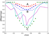 |
Fig. 2 Light curves for models A (red triangles), B (blue triangles), and C (green triangles) in Table 1. These curves are able to explain the typical values of Δmag seen in the TESS LC (see text and Fig. 1). Model A reproduces dips with Δmag = 0.1, model B for Δmag = 0.2, and model C for Δmag = 0.7. We also include LCs formed with spots covering a fraction of the stellar surface (red and blue plus signs). For comparison, we include the features at JD 60 2240 (magenta line) and JD 60 244 (cyan line) in the TESS LC. |
5 Conclusions
We interpreted the dipper-like TESS LC of UX Tau A (Espaillat et al. 2024) using the dusty magnetospheric stream model described in Nagel & Bouvier (2020) and Nagel et al. (2024). We used the magnetospheric configuration derived from the Hα profile fitting by Espaillat et al. (2024) as the backbone where the dust that blocks part of the stellar radiation is located. We took the values of Ṁ from the fit. We computed a grid of models with the given ranges of Ṁ, i, Rmag, and Wr. According to the physical interpretation of Espaillat et al. (2024), the amount of material arriving to the inner disk from the outer disk in the pre-TD surrounding the star varies over a depletion timescale of 0.1 yr. The dusty magnetosphere scenario lead us to add amax and ζd in the set of fitting parameters.
The main conclusions are as follows:
Magnetospheres with Rmag < 4.8 R⋆ are too hot for the dust to survive. We therefore discarded these models, restricting the consistent models to a subset of 17 cases out of 192.
If we assume that the period associated with the LC is the stellar rotational period, Prot = 3.8 d, then Rco ≳ Rmag and the system cannot be cataloged in the strong or weak propeller regime (Romanova et al. 2018). This means that a disk wind (Shu et al. 2000) as the mechanism responsible for moving dust to the required heights to produce dips (Gaidos et al. 2024) is not present.
A warp at Rmag formed with the interaction of the disk and the magnetosphere is able to explain dippers where i > 60∘ (Bouvier et al. 1999; McGinnis et al. 2015; Nagel & Bouvier 2019). Since i < 60∘ in this case from the Hα fitting (Espaillat et al. 2024), the TESS LC cannot be easily described with an inner disk warp.
We therefore conclude that the presence of dusty magnetospheric streams (Nagel & Bouvier 2020; Nagel et al. 2024) is a tentative scenario to interpret the TESS LC of UX Tau A.
We derived at least three models for the observed LC consistent with three different stages of the dusty magnetosphere models: the low (Δmag ∼ 0.1), the middle (Δmag ∼ 0.2), and the high (Δmag ∼ 0.7) cases. For all the cases we used Ṁ = 3 × 10⁻⁸ and Rmag = 5.6 R⋆. In the first case: i = 52∘, amax = 0.143 cm, and ζd = 0.01. In the second case: i = 56∘, amax = 0.0979 cm, and ζd = 0.01. In the third case: i = 60∘, amax = 0.143 cm, and ζd = 0.012. These are not the only models consistent with the observations, as the interplay between Ṁ, amax and ζd defines a region in the parameter space where the same amount of dust opacity occurs along the line of sight. The mid-infrared excess estimated in Espaillat et al. (2024) is consistent with an optically thick inner disk at 1550 K with a lower limit of dust mass of 10−11 M⊙. This amount of material is enough to sustain a ∼ 10−8 M⊙ yr−1 flow of material to the star for a few days as required for the models.
The low and middle cases can also be interpreted with spots at a latitude of 45∘. For the first case, the size of the spot is As = 0.005 with temperature Ts = 122124 K. For the second case, the size of the spot is As = 0.02 with temperature Ts = 8837 K. This means that a scenario with multiple mechanisms is likely.
In a highly dynamic environment, the characterization of the innermost regions of the disk becomes important to describe dusty configurations likely to produce dips in LCs. The misalignment between the inner and outer disks in pre-TD (Bohn et al. 2022; Sicilia-Aguilar et al. 2020) is a configuration leading to the precession of the inner disk. In such a scenario, the depths of the dips are changing on a timescale that should be defined with detailed simulations addressing this issue.
Acknowledgements
E.N. acknowledges the support of the University of Guanajuato where this article was written. This project has received funding from the European Research Council (ERC) under the European Union’s Horizon 2020 research and innovation programme (Grant Agreement no. 742095; SPIDI: Star-Planets-Inner Disk-Interactions, https://www.spidi-eu.org).
References
- Alencar, S. H. P., Teixeira, P. S., Guimarães, M. M., et al. 2010, A&A, 519, A88 [NASA ADS] [CrossRef] [EDP Sciences] [Google Scholar]
- Alencar, S. H. P., Bouvier, J., Donati, J.-F., et al. 2018, A&A, 620, A195 [NASA ADS] [CrossRef] [EDP Sciences] [Google Scholar]
- Blandford, R. D., & Payne, D. G. 1982, MNRAS, 199, 883 [CrossRef] [Google Scholar]
- Bohn, A. J., Benisty, M., Perraut, K., et al. 2022, A&A, 658, A183 [NASA ADS] [CrossRef] [EDP Sciences] [Google Scholar]
- Bouvier, J., Chelli, A., Allain, S., et al. 1999, A&A, 349, 619 [NASA ADS] [Google Scholar]
- Cody, A. M., & Hillenbrand, L. 2018, AJ, 156, 71 [Google Scholar]
- Doi, K., Kataoka, A., Liu, H. B., et al. 2024, ApJ, 974, L25 [Google Scholar]
- Espaillat, C., D’Alessio, P., Hernández, J., et al. 2010, ApJ, 717, 441 [Google Scholar]
- Espaillat, C., Furlan, E., D’Alessio, P., et al. 2011, ApJ, 728, 49 [NASA ADS] [CrossRef] [Google Scholar]
- Espaillat, C. C., Thanathibodee, T., Zhu, Z., et al. 2024, ApJ, 973, L16 [Google Scholar]
- Flaherty, K. M., Muzerolle, J., Rieke, G., et al. 2012, ApJ, 748, 71 [NASA ADS] [Google Scholar]
- Gaidos, E., Thanathibodee, T., Hoffman, A., et al. 2024, ApJ, 966, 167 [NASA ADS] [CrossRef] [Google Scholar]
- GRAVITY Collaboration (Soulain, A., et al.) 2023, A&A, 674, A203 [NASA ADS] [CrossRef] [EDP Sciences] [Google Scholar]
- Hartmann, L., Hewett, R., & Calvet, N. 1994, ApJ, 426, 669 [Google Scholar]
- Ingleby, L., Calvet, N., Herczeg, G., et al. 2013, ApJ, 767, 112 [Google Scholar]
- Ingleby, L., Espaillat, C., Calvet, N., et al. 2015, ApJ, 805, 149 [NASA ADS] [CrossRef] [Google Scholar]
- Kesseli, A. Y., Petkova, M. A., Wood, K., et al. 2016, ApJ, 828, 42 [NASA ADS] [CrossRef] [Google Scholar]
- Konigl, A. 1989, ApJ, 342, 208 [NASA ADS] [Google Scholar]
- Kulkarni, A. K., & Romanova, M. M. 2013, MNRAS, 433, 3048 [NASA ADS] [CrossRef] [Google Scholar]
- Kurosawa, R., & Romanova, M. M. 2013, MNRAS, 431, 2673 [Google Scholar]
- Li, R., Chen, Y.-X., & Lin, D. N. C. 2022, MNRAS, 510, 5246 [NASA ADS] [CrossRef] [Google Scholar]
- Liffman, K., Bryan, G., Hutchison, M., & Maddison, S. T. 2020, MNRAS, 493, 4022 [CrossRef] [Google Scholar]
- Mathis, J. S., Rumpl, W., & Nordsieck, K. H. 1977, ApJ, 217, 425 [Google Scholar]
- McGinnis, P. T., Alencar, S. H. P., Guimaraes, M. M., et al. 2015, A&A, 577, A11 [NASA ADS] [CrossRef] [EDP Sciences] [Google Scholar]
- Morales-Calderón, M., Stauffer, J. R., Hillenbrand, L. A., et al. 2011, ApJ, 733, 50 [CrossRef] [Google Scholar]
- Nagel, E., & Bouvier, J. 2019, A&A, 625, A45 [NASA ADS] [CrossRef] [EDP Sciences] [Google Scholar]
- Nagel, E., & Bouvier, J. 2020, A&A, 643, A157 [EDP Sciences] [Google Scholar]
- Nagel, E., & Bouvier, J. 2023, MNRAS, 524, 1997 [NASA ADS] [Google Scholar]
- Nagel, E., Bouvier, J., & Duarte, A. E. 2024, A&A, 688, A61 [NASA ADS] [CrossRef] [EDP Sciences] [Google Scholar]
- Pinilla, P., Benisty, M., Waters, R., Bae, J., & Facchini, S. 2024, A&A, 686, A135 [NASA ADS] [CrossRef] [EDP Sciences] [Google Scholar]
- Ribas, A., Clarke, C. J., & Zagaria, F. 2024, MNRAS, 532, 1752 [NASA ADS] [CrossRef] [Google Scholar]
- Roggero, N., Bouvier, J., Rebull, L. M., & Cody, A. M. 2021, A&A, 651, A44 [NASA ADS] [CrossRef] [EDP Sciences] [Google Scholar]
- Romanova, M. M., Ustyugova, G. V., Koldoba, A. V., & Lovelace, R. V. E. 2013, MNRAS, 430, 699 [Google Scholar]
- Romanova, M. M., Blinova, A. A., Ustyugova, G. V., Koldoba, A. V., & Lovelace, R. V. E. 2018, New Astron., 62, 94 [Google Scholar]
- Shu, F. H., Najita, J. R., Shang, H., & Li, Z.-Y. 2000, Protostars and Planets IV, eds. V. Mannings, A. P. Boss, & S. S. Russell (Tucson: University of Arizona Press), 789 [Google Scholar]
- Sicilia-Aguilar, A., Manara, C. F., de Boer, J., et al. 2020, A&A, 633, A37 [NASA ADS] [CrossRef] [EDP Sciences] [Google Scholar]
- Takasao, S., Tomida, K., Iwasaki, K., & Suzuki, T. K. 2022, ApJ, 941, 73 [NASA ADS] [CrossRef] [Google Scholar]
- Tessore, B., Soulain, A., Pantolmos, G., et al. 2023, A&A, 671, A129 [NASA ADS] [CrossRef] [EDP Sciences] [Google Scholar]
- Thanathibodee, T., Molina, B., Serna, J., et al. 2023, ApJ, 944, 90 [NASA ADS] [CrossRef] [Google Scholar]
- Wojtczak, J. A., Tessore, B., Labadie, L., et al. 2024, A&A, 689, A124 [NASA ADS] [CrossRef] [EDP Sciences] [Google Scholar]
- Xu, S., Rappaport, S., van Lieshout, R., et al. 2018, MNRAS, 474, 4795 [Google Scholar]
All Tables
Parameters of the grid of models presented in this work with Δmag > 0.001, analyzed to describe their behavior.
Parameters of the models that fit the three typical observed amplitudes presented in this work.
All Figures
|
Fig. 1 Light curve from TESS during Sector 70 and the first part of Sector 71 as in Espaillat et al. (2024). The high-amplitude dips at JD 60 2240 and JD 60 2244 are clearly seen. |
| In the text | |
|
Fig. 2 Light curves for models A (red triangles), B (blue triangles), and C (green triangles) in Table 1. These curves are able to explain the typical values of Δmag seen in the TESS LC (see text and Fig. 1). Model A reproduces dips with Δmag = 0.1, model B for Δmag = 0.2, and model C for Δmag = 0.7. We also include LCs formed with spots covering a fraction of the stellar surface (red and blue plus signs). For comparison, we include the features at JD 60 2240 (magenta line) and JD 60 244 (cyan line) in the TESS LC. |
| In the text | |
Current usage metrics show cumulative count of Article Views (full-text article views including HTML views, PDF and ePub downloads, according to the available data) and Abstracts Views on Vision4Press platform.
Data correspond to usage on the plateform after 2015. The current usage metrics is available 48-96 hours after online publication and is updated daily on week days.
Initial download of the metrics may take a while.