| Issue |
A&A
Volume 643, November 2020
|
|
|---|---|---|
| Article Number | A5 | |
| Number of page(s) | 17 | |
| Section | Extragalactic astronomy | |
| DOI | https://doi.org/10.1051/0004-6361/202038231 | |
| Published online | 27 October 2020 | |
The ALPINE-ALMA [C II] survey
Molecular gas budget in the early Universe as traced by [C II]
1
Observatoire de Genève, Université de Genève, 51 Ch. des Maillettes, 1290 Versoix, Switzerland
e-mail: This email address is being protected from spambots. You need JavaScript enabled to view it.
2
Università di Bologna – Dipartimento di Fisica e Astronomia, Via Gobetti 93/2, 40129 Bologna, Italy
3
INAF – Osservatorio di Astrofisica e Scienza dello Spazio di Bologna, Via Gobetti 93/3, 40129 Bologna, Italy
4
Aix Marseille Université, CNRS, LAM (Laboratoire d’Astrophysique de Marseille) UMR 7326, 13388 Marseille, France
5
The Cosmic Dawn Center, University of Copenhagen, Vibenshuset, Lyngbyvej 2, 2100 Copenhagen, Denmark
6
Niels Bohr Institute, University of Copenhagen, Lyngbyvej 2, 2100 Copenhagen, Denmark
7
Kavli Institute for the Physics and Mathematics of the Universe, The University of Tokyo (Kavli IPMU, WPI), 277-8583 Kashiwa, Japan
8
Department of Astronomy, School of Science, The University of Tokyo, 7-3-1 Hongo, Bunkyo, Tokyo, 113-0033
Japan
9
Cavendish Laboratory, University of Cambridge, 19 J. J. Thomson Ave., Cambridge, CB3 0HE
UK
10
Kavli Institute for Cosmology, University of Cambridge, Madingley Road, Cambridge, CB3 0HA
UK
11
Leiden Observatory, Leiden University, PO Box 9500, 2300 RA Leiden, The Netherlands
12
IPAC, M/C 314-6, California Institute of Technology, 1200 East California Boulevard, Pasadena, CA, 91125
USA
13
Max-Planck-Institut für Astronomie, Königstuhl 17, 69117 Heidelberg, Germany
14
Dipartimento di Fisica e Astronomia, Università di Padova, Vicolo dell’Osservatorio, 3, 35122 Padova, Italy
15
INAF – Osservatorio Astronomico di Padova, Vicolo dell’Osservatorio 5, 35122 Padova, Italy
16
The Caltech Optical Observatories, California Institute of Technology, Pasadena, CA, 91125
USA
17
Instituto de Investigación Multidisciplinar en Ciencia y Tecnología, Universidad de La Serena, Raúl Bitrán, 1305 La Serena, Chile
18
Departamento de Astronomía, Universidad de La Serena, Av. Juan Cisternas 1200 Norte, La Serena, Chile
19
Centro de Astronomía (CITEVA), Universidad de Antofagasta, Avenida Angamos 601, Antofagasta, Chile
20
INAF – Osservatorio Astrofisico di Arcetri, Largo E. Fermi 5, 50125 Firenze, Italy
21
Space Telescope Science Institute, 3700 San Martin Drive, Baltimore, MD, 21218
USA
22
Instituto de Física y Astronomía, Universidad de Valparaíso, Avda. Gran Bretaña 1111, Valparaíso, Chile
23
Department of Physics, University of California, Davis, One Shields Ave., Davis, CA, 95616
USA
24
Department of Astronomy, University of Florida, 211 Bryant Space Sciences Center, Gainesville, FL, 32611
USA
Received:
22
April
2020
Accepted:
17
July
2020
Abstract
The molecular gas content of normal galaxies at z > 4 is poorly constrained because the commonly used molecular gas tracers become hard to detect at these high redshifts. We use the [C II] 158 μm luminosity, which was recently proposed as a molecular gas tracer, to estimate the molecular gas content in a large sample of main sequence star-forming galaxies at z = 4.4 − 5.9, with a median stellar mass of 109.7 M⊙, drawn from the ALMA Large Program to INvestigate [C II] at Early times survey. The agreement between the molecular gas masses derived from [C II] luminosities, dynamical masses, and rest-frame 850 μm luminosities extrapolated from the rest-frame 158 μm continuum supports [C II] as a reliable tracer of molecular gas in our sample. We find a continuous decline of the molecular gas depletion timescale from z = 0 to z = 5.9, which reaches a mean value of (4.6 ± 0.8) × 108 yr at z ∼ 5.5, only a factor of between two and three shorter than in present-day galaxies. This suggests a mild enhancement of the star formation efficiency toward high redshifts. Our estimates also show that the previously reported rise in the molecular gas fraction flattens off above z ∼ 3.7 to achieve a mean value of 63%±3% over z = 4.4 − 5.9. This redshift evolution of the gas fraction is in line with that of the specific star formation rate. We use multi-epoch abundance-matching to follow the gas fraction evolution across cosmic time of progenitors of z = 0 Milky Way-like galaxies in ∼1013 M⊙ halos and of more massive z = 0 galaxies in ∼1014 M⊙ halos. Interestingly, the former progenitors show a monotonic increase of the gas fraction with redshift, while the latter show a steep rise from z = 0 to z ∼ 2 followed by a constant gas fraction from z ∼ 2 to z = 5.9. We discuss three possible effects, namely outflows, a pause in gas supply, and over-efficient star formation, which may jointly contribute to the gas fraction plateau of the latter massive galaxies.
Key words: galaxies: evolution / galaxies: high-redshift / galaxies: ISM / ISM: molecules
© ESO 2020
1. Introduction
As cold molecular hydrogen, H2, is the fuel for star formation, it is necessary to probe the molecular gas content of galaxies with cosmic time to understand their stellar mass assembly. With an increasing number of normal star-forming galaxies (SFGs) for which measurements of cold molecular gas mass (Mmolgas) are available, we are starting to bring to light the significant role that molecular gas plays in the evolution of these galaxies, which contribute to about 90% of the cosmic star formation rate (SFR) density. SFGs are found to follow the star-forming main sequence (MS), a tight relation between stellar mass (Mstars) and SFR, which evolves with redshift and has a dispersion of about ±0.3 dex (e.g., Rodighiero et al. 2011; Speagle et al. 2014; Whitaker et al. 2014; Tasca et al. 2015; Faisst et al. 2016). The redshift evolution of the MS is such that, at a given Mstars, high-redshift galaxies form more stars per unit time than low-redshift galaxies, which results in a strong increase in the specific star formation rate (sSFR = SFR/Mstars) with redshift. It is now well established that, up to z ∼ 2.5, the sSFR increase is linked to the observed rise of the molecular gas content of galaxies with redshift (e.g., Saintonge et al. 2013; Genzel et al. 2015; Dessauges-Zavadsky et al. 2017; Tacconi et al. 2018, 2020; Decarli et al. 2019). Likewise, the location of a galaxy in the SFR–Mstars plane is primarily governed by its supply (mass) of molecular gas and to some extent also its star formation efficiency (SFE = SFR/Mmolgas) (e.g., Magdis et al. 2012; Dessauges-Zavadsky et al. 2015; Genzel et al. 2015; Silverman et al. 2015, 2018; Scoville et al. 2016; Tacconi et al. 2020).
To explain the high SFR and Mmolgas of SFGs in the early Universe, it has been proposed that they are sustained with cold gas accreted from the cosmic web (e.g., Kere et al. 2005; Dekel et al. 2009). In this context, the MS may be interpreted in terms of a “bathtub” model, in which MS galaxies lie in a quasi-steady state equilibrium whereby star formation is regulated by the available gas reservoir, and whose content is replenished through pristine gas accretion flows and is eventually diminished by the amount of material galaxies return to the intergalactic medium through outflows (e.g., Bouché et al. 2010; Davé et al. 2011, 2012; Lilly et al. 2013; Dekel & Mandelker 2014). In addition to the average stellar mass growth of SFGs along the MS, simulations suggest SFGs oscillate up and down in sSFR across the MS dispersion, owing to feedback effects that alter the gas accretion rate; internal gas transport; and compaction events (Tacchella et al. 2016; Orr et al. 2019). The bathtub model agrees with most of the scaling relations observed for MS SFGs, such as the Kennicutt–Schmidt (KS) star-formation law (Kennicutt 1998a; Tacconi et al. 2013) and the mass–metallicity relation (e.g., Erb et al. 2006; Maiolino et al. 2008; Mannucci et al. 2010; Ginolfi et al. 2020a), and with the dynamically more turbulent galactic disks at high-redshift (e.g., Förster Schreiber et al. 2009; Wisnioski et al. 2015; Molina et al. 2017; Girard et al. 2018).
While H2 is the most abundant molecule in the Universe, it is nevertheless difficult to detect in cold media because it features no emission lines with excitation temperatures below 100 K. Fortunately, the cold molecular gas is not pure H2, but contains heavier elements, like carbon and oxygen, and is mixed with dust grains. Therefore, three indirect cold H2 tracers are commonly used to estimate the H2 content of high-redshift galaxies: the CO molecule rotational transitions (Bolatto et al. 2013, and references therein); the dust mass inferred from the fit of the thermal far-infrared (FIR) dust spectral energy distribution (SED; e.g., Leroy et al. 2011; Magdis et al. 2011; Santini et al. 2014; Béthermin et al. 2015; Kaasinen et al. 2019); and the cold dust continuum emission measured in the Rayleigh-Jeans tail regime of the FIR SED (e.g., Scoville et al. 2014, 2016, 2017). The Plateau de Bure interferometer – now the Northern Extended Millimeter Array (NOEMA) – and the Atacama Large Millimeter/sub-millimeter Array (ALMA) have largely contributed to the census of Mmolgas in MS SFGs over the peak of the cosmic star formation history from z = 0 to z ∼ 3.5 (e.g., Daddi et al. 2010a; Magnelli et al. 2012; Tacconi et al. 2013, 2018; Saintonge et al. 2013, 2017; Santini et al. 2014; Dessauges-Zavadsky et al. 2015; Schinnerer et al. 2016; Decarli et al. 2019; Liu et al. 2019b). At higher redshifts, both CO and dust become harder to detect, because of (i) the surface brightness dimming as (1 + z)4, (ii) the lower metallicities expected in distant galaxies making CO dark and dust rare, and (iii) the ALMA bands only covering high (J ≥ 5) CO transitions at z > 4.5, which requires knowledge of the CO excitation state and gas density to determine the total Mmolgas. Therefore, only two Mmolgas estimates derived from CO luminosity measurements have been reported in MS SFGs at z > 5.5 to date (D’Odorico et al. 2018; Pavesi et al. 2019). Furthermore, the dozens of Mmolgas measurements derived from FIR dust continuum for MS SFGs at z > 4 (Scoville et al. 2016; Liu et al. 2019b) are largely biased toward massive galaxies with Mstars ≳ 1011.5 M⊙ (and hence high SFRs).
Clearly, the MS is not yet adequately covered at these high redshifts (see the right panel of Fig. 4 of Liu et al. 2019b): for a large parameter space of Mstars and SFR, molecular gas masses of MS SFGs at z > 4 still need to be accessed to establish how gas reservoirs and gas consumption timescales change as a function of at least three fundamental parameters, namely cosmic time, Mstars, and SFR. The study of the molecular gas content of galaxies in the range 4 < z < 6 is all the more important as this redshift range corresponds to the key evolutionary phase in the early life of galaxies, between their primordial and mature phases, during which many fundamental properties of present-day galaxies are established (Ribeiro et al. 2016; Feldmann 2015). During this early phase, galaxies are known to double their Mstars at rates that are five to ten times higher than at later cosmic times (Faisst et al. 2016; Davidzon et al. 2018), which may require very efficient star formation and/or a considerable supply of molecular gas.
The C+ radiation, which is considered to be an important coolant of the neutral interstellar medium (ISM), is accessible through the [C II] line at 158 μm (one of the strongest lines in the FIR spectra; see Carilli & Walter 2013), and was shown to correlate with the total integrated SFR of galaxies (e.g., De Looze et al. 2011, 2014; Schaerer et al. 2020) and spatially resolved SFR (Pineda et al. 2014; Herrera-Camus et al. 2015). The C+ radiation has also been found to be a good tracer of molecular gas at 0.03 < z < 0.2 by Hughes et al. (2017a), and more recently over 0 < z < 6 by Zanella et al. (2018). Such a correlation between [C II] luminosity (LCII) and Mmolgas can be exploited to overcome the observational challenge of detecting CO or FIR dust emission in very high-redshift normal SFGs. In this context, our recently completed ALMA Large Program to INvestigate [C II] at Early times (ALPINE; Le Fèvre et al. 2020; Béthermin et al. 2020; Faisst et al. 2020) delivers the first large sample of 75 [C II] emission detections and 43 upper limits obtained for a representative population of ultraviolet (UV)-selected MS SFGs at z = 4.4 − 5.9 with SFR ≳ 10 M⊙ yr−1 and Mstars = 108.4 − 1011 M⊙. Relying on the Zanella et al. (2018) correlation, we use ALPINE data to provide the first set of molecular gas mass estimates for MS SFGs at z = 4.4 − 5.9.
In Sect. 2 we summarise the ALPINE survey, the physical properties of galaxies in our survey, and the ALMA observations. Measurements of molecular gas masses obtained using [C II] luminosity are presented in Sect. 3, together with specific tests of [C II] as a reliable molecular gas tracer for the ALPINE galaxies. In Sect. 4 we describe the comparison sample, which includes lower redshift MS SFGs with molecular gas masses determined from CO luminosities. We argue that CO-detected MS SFGs represent a better comparison sample for the ALPINE galaxies with respect to FIR continuum-detected SFGs with typically larger Mstars. In Sect. 5 we discuss the inferred molecular gas depletion timescales and molecular gas fractions, which we compare to those of lower redshift CO-detected galaxies. The evolution of the molecular gas fraction across cosmic time is described in Sect. 5.4. We use the multi-epoch abundance-matching predictions to connect the progenitors at high redshift with their descendants at z = 0. Our main results are summarized in Sect. 6.
Throughout the paper, we assume the ΛCDM cosmology with Ωm = 0.3, ΩΛ = 0.7 and H0 = 70 km s−1 Mpc−1, and we adopt the Chabrier (2003) initial mass function.
2. Observations and physical properties of ALPINE galaxies
The 118 targeted galaxies from the ALPINE survey (Le Fèvre et al. 2020 – survey paper; Béthermin et al. 2020 – data reduction paper; Faisst et al. 2020 – ancillary data paper) are UV-selected galaxies from the COSMic evOlution Survey (COSMOS, 105 galaxies; Scoville et al. 2007) and the Extended Chandra Deep Field South survey (ECDFS, 13 galaxies; Giacconi et al. 2002). Optical spectroscopy data are available for all galaxies, ensuring reliable rest-frame UV spectroscopic redshift measurements, and they all benefit from multi-wavelength ground- and space-based imaging from UV to IR.
The detailed description of the ancillary spectra and photometric data can be found in Faisst et al. (2020), together with the redshift measurements and the SED fits. The derived Mstars and SFR of ALPINE galaxies are in the range of Mstars = 108.4 − 1011 M⊙ and SFRSED = 3 − 630 M⊙ yr−1, respectively, and follow the expected MS at z ∼ 5. There is good agreement between SFRSED and SFRUV + IR, as shown by Schaerer et al. (2020). The latter corresponds to the sum of SFRUV, measured from the UV luminosity at 1500 Å rest-frame (uncorrected for dust attenuation), and SFRIR, measured from the rest-frame 158 μm dust continuum emission flux and the FIR SED template of Béthermin et al. (2017) to infer the total IR luminosity (LIR) integrated between 8 μm and 1000 μm, as described in Béthermin et al. (2020). Throughout the paper, we adopt the Mstars listed in Table A.1 of Faisst et al. (2020) with a typical uncertainty of ∼0.15 dex and obtained based on photometry that includes the Spitzer IR imaging. The SFRUV + IR values are derived from the UV magnitudes listed in Table A.1 of Faisst et al. (2020) and LIR given in Table B.1 of Béthermin et al. (2020). For galaxies undetected in the FIR dust continuum (95 ALPINE galaxies), we consider only SFRUV as the total SFR throughout the paper. Schaerer et al. (2020) provide a detailed discussion of the possible amount of SFRIR (the dust-obscured star formation rate) in these 95 ALPINE galaxies and find that their total SFR can be underestimated by a factor of 1.6, on average, according to the average empirically calibrated relation between IR excess (IRX = LIR/LUV) and UV spectral slope (β; fλ ∝ λβ), which was derived by Fudamoto et al. (2020) for the ALPINE sample from median stacking of individual continuum images in bins of β. However, for the majority of the 95 ALPINE galaxies, SFRIR was found to be small (≲40% of SFRUV), since the UV spectral slope obtained by these latter authors is relatively blue. We would like to mention here that none of our conclusions change when a possible underestimation of the total SFR is taken into account.
The ALMA observations were carried out in band 7 during Cycles 5 and 6, and completed in February 2019. Band 7 (275 − 373 GHz) covers the [C II] 158 μm line from z = 4.1 to z = 5.9, but to avoid an atmospheric absorption, no source was included in the redshift range of z = 4.6 − 5.1. Each target was observed for 15 − 25 min of on-source time, with the phase center positioned at the rest-frame UV position of the target and one spectral window in the lower-frequency sideband tuned to the [C II] frequency redshifted by the rest-frame UV spectroscopic redshift of that target (Faisst et al. 2020). The other three spectral windows were used for the FIR continuum around 158 μm rest-frame, close to the FIR SED peak. The ALMA visibility calibration, cleaning, and imaging were performed using the Common Astronomy Software Applications package (CASA; McMullin et al. 2007), as described in detail in Béthermin et al. (2020). The resulting root-mean-square noise (rms) of the 118 [C II] data cubes ranges between 0.2 mJy beam−1 and 0.55 mJy beam−1 per 25 km s−1 channel for an angular resolution varying between 0.72″ (minimum minor axis) and 1.6″ (maximum major axis). The continuum sensitivity varies with frequency. We reach a mean rms of 50 μJy beam−1 for the ALPINE galaxies at z = 4.4 − 4.6, and 28 μJy beam−1 for the ALPINE galaxies at z = 5.1 − 5.9. The ALMA dataset leads to robust [C II] emission detections for 75 ALPINE galaxies and robust FIR dust continuum emission detections for 23 ALPINE galaxies, with a signal-to-noise ratio (S/N) larger than 3.5 corresponding to 95% purity threshold of both the [C II] line and FIR continuum (Béthermin et al. 2020). Throughout the paper, we consider the 2σ-clipped [C II] fluxes1, and the FIR continuum fluxes derived using the 2D elliptical Gaussian fits. For the 43 ALPINE targets for which no [C II] detections are available, we consider the “secure” 3σ upper limits2 on [C II] fluxes listed in Table C2 of Béthermin et al. (2020).
At the achieved angular resolutions, with an average circularized beam of 0.9″ corresponding to ∼5.3 − 6.1 kpc at z = 4.4 − 5.9, about 2/3 of the ALPINE [C II]-detected galaxies are moderately spatially resolved in the [C II] velocity-integrated intensity maps (Béthermin et al. 2020; Le Fèvre et al. 2020; Fujimoto et al. 2020), meaning their intrinsic (total) sizes as seen in [C II] emission are about the size of the beam, or a significant fraction thereof, as illustrated by the spectacular object studied by Jones et al. (2020). A large diversity of [C II] emission morphologies is observed, from compact and/or unresolved objects, through objects appearing as very extended (Fujimoto et al. 2020; Ginolfi et al. 2020b), to objects showing double (or more) merger-like components (Jones et al. 2020). From our morpho-kinematic visual classification based on the [C II] emission and velocity field and multi-band optical to IR images, which is described in Le Fèvre et al. (2020), we find signatures of possibly interacting systems for 31 ALPINE [C II]-detected galaxies, while only 9 ALPINE galaxies are likely rotation-dominated. This indicates that mass assembly through merging processes is frequent at these redshifts for MS SFGs. In what follows, we exclude the 31 galaxies classified as mergers in order to work with a sample of galaxies where robust measurements of their physical properties can be determined, since deblending the [C II] and dust continuum emissions in closely interacting multi-component systems is difficult with the available ALMA data (Béthermin et al. 2020). Therefore, our final sample consists of 87 ALPINE galaxies; of these 44 are detected in [C II], while for 43, only [C II] upper limits are available.
3. Molecular gas mass estimates
3.1. [C II] as a tracer of cold molecular gas
Zanella et al. (2018) proposed the [C II] emission as a reliable tracer of molecular gas by finding a tight empirical correlation, with a 0.3 dex dispersion, between the [C II] luminosity and molecular gas mass derived using mainly the CO tracer (see also Hughes et al. 2017a). Zanella et al. (2018) investigated whether this relation holds with the nature of galaxies (MS galaxies, starbursts offset from the MS), redshift (from z = 0 to z = 6), and metallicity (from 12 + log(O/H) = 7.9 to 12 + log(O/H) = 8.8), and observed that globally it does, but with a larger scatter in the αCII = Mmolgas/LCII conversion factor for galaxies above the MS, and with metallicities 12 + log(O/H)≲8.4. These latter authors also proposed to use their findings to interpret the LCII/LIR deficit observed in ultra-luminous IR galaxies (ULIRGs) and high-redshift starbursts. Indeed, if LCII traces Mmolgas (and LIR the SFR), then the [C II] deficit reflects shorter molecular gas depletion timescales in ULIRGs and distant starbursts, which is consistent with measurements (e.g., Daddi et al. 2010b; Genzel et al. 2010; Combes et al. 2013; Silverman et al. 2018). However, the origin of the [C II] deficit is complex, and can also be driven by conditions external to star formation, such as AGN activity (e.g., Sargsyan et al. 2012; Herrera-Camus et al. 2018).
From the theoretical point of view, the origin of the emission of [C II] is complex, because different ISM phases – ionized, neutral, and molecular – are contributing to it. As a result, one needs to establish whether the fraction of [C II] emission arising from photodissociation regions (PDRs; Stacey et al. 1991; Malhotra et al. 2001; Cormier et al. 2015; Diaz-Santos et al. 2017), which are produced by the UV radiation from hot stars heating the outer layers of molecular clouds and associated with both the interface layer of neutral gas as well as ionized gas in the H II region itself, is dominating (or not dominating) that arising from the CO photodissociation into C and C+ in the cold neutral medium of molecular clouds (Maloney & Black 1988; Madden et al. 1993; Wolfire et al. 2010; Narayanan & Krumholz 2017). In the PDR case, C+ is rather tracing star formation, while in the CO photodissociation case C+ emission emerges from the molecular phase.
The [C II] line has raised considerable interest in galaxies at z ≳ 5, leading several authors to produce numerical simulations to model [C II] and to suggest that its emission is dominated at the level of > 60 − 85% by molecular clouds more than by diffuse ionized gas (Vallini et al. 2015; Pallottini et al. 2017; Accurso et al. 2017; Olsen et al. 2018). Indeed, CO and [C II] emission maps of the high-redshift galaxy simulated by Vallini et al. (2018) and Pallottini et al. (2017), respectively, clearly show the same morphology with similar spatial distributions at a scale of 30 pc. In the Milky Way, dense PDRs and CO-dark H2 gas are also the dominant [C II] emitters, and are responsible for ∼55% of the total [C II] emission, while the diffuse ionized gas and diffuse neutral gas contribute ∼20% and ∼25%, respectively (Pineda et al. 2014; and see also the simulation predictions from Li et al. 2018). Similarly, in nearby galaxies, the [C II] emission arises mainly from PDRs and the contribution from the ionized gas phases is typically ≲30% of the observed emission (Abdullah et al. 2017; Croxall et al. 2017; Cormier et al. 2019), although the fraction of [C II] originating in the cooler ionized gas appears to increase with gas-phase metallicity. As Zanella et al. (2018) warn, when using [C II] as a molecular gas tracer one needs to be aware that because the C+ emission might not fully emerge from one single gas phase, the measured [C II] luminosity might lead to an overestimation of the luminosity arising from the molecular gas. On the other hand, as C+ is emitted only in regions where star formation is taking place, the molecular gas not illuminated by stars would be undetected. Finally, [C II] emission is also found in the outer parts of nearby galaxies, where low-density H II regions were reported to contribute up to ∼50% of the extended [C II] emission (Madden et al. 1993; see also Langer et al. 2016, 2018 for their studies of the Milky Way). More recently, [C II] emission has also been observed in the outer parts of high-redshift SFGs (Fujimoto et al. 2019; Ginolfi et al. 2020b). In the case of the ALPINE nonmerger galaxies, Fujimoto et al. (2020) find that only a small fraction of them, namely 7 out of 44 or ∼15%, show a non-negligible [C II] halo component extended on scales of ≳10 − 15 kpc. From the stacking analysis of the full sample of ALPINE nonmergers, Ginolfi et al. (2020c) estimate an average flux contribution of the extended [C II] halo component of ∼10% with respect to the total [C II] flux. We therefore argue that the contribution from the halo component to the [C II] luminosities used in the present study (measured as discussed in Sect. 2) must be negligible for the bulk of the ALPINE galaxies.
Applying the calibration of Zanella et al. (2018) between [C II] luminosity and molecular gas mass, namely
 (1)
(1)
to the 44 ALPINE [C II]-detected nonmerger galaxies with log(LCII/L⊙) = 7.8 − 9.2 in the regime tested by Zanella et al. (2018), we obtain molecular gas masses in the range of  for these MS SFGs at z = 4.4 − 5.9, as shown by the
  distribution in Fig. 1. We calculate the error bars on the [C II]-estimated molecular gas masses by summing in quadrature the relative uncertainty on [C II] fluxes (see Béthermin et al. 2020) and the 0.3 dex dispersion of the LCII–
 calibration (Zanella et al. 2018).
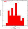 |
Fig. 1. Distribution of molecular gas masses of the 44 ALPINE [C II]-detected nonmerger galaxies at z = 4.4 − 5.9. The molecular gas masses were derived using the calibration of Zanella et al. (2018) between [C II] luminosity and molecular gas mass (Eq. (1)). |
3.2. Other cold molecular gas mass tracers
In what follows, for a subset of the ALPINE sample we cross-correlate the [C II]-derived molecular gas mass estimates with molecular gas masses inferred using other molecular gas tracers to check the robustness of [C II] as the tracer of cold molecular gas in our sample of 4.4 < z < 5.9 MS SFGs. Moreover, beyond this check, we provide the first step toward an independent LCII–Mmolgas calibration based on dynamical masses (see Sect. 3.2.3).
3.2.1. The IR luminosity versus CO luminosity relation
We can use the well-established empirical relation between IR luminosity and CO(1–0) luminosity measurements (Daddi et al. 2010a; Carilli & Walter 2013; Sargent et al. 2014; Dessauges-Zavadsky et al. 2015) to test whether or not the derived  agree with the measured LIR along the expected relation. This relation, which spans almost five orders of magnitude in LIR from 109 L⊙ to 1013.5 L⊙, was found to be valid for a variety of galaxy types, namely MS galaxies, starbursts, and mergers at redshifts between z = 0 and z ∼ 5.3. In Fig. 2 we show the IR luminosities measured for 11 ALPINE [C II]-detected nonmerger galaxies as a function of the CO(1–0) luminosities inferred from the [C II] molecular gas masses and a range of CO-to-H2 conversion factors (αCO) from the Milky Way value of 4.36 M⊙ (K km s−1 pc2)−1 to the starburst value of 1 M⊙ (K km s−1 pc2)−1 (Bolatto et al. 2013). We find that for the Milky Way CO-to-H2 conversion factor, all ALPINE galaxies fall within the 0.38 dex dispersion of the IR luminosity versus CO(1–0) luminosity relation,
  , calibrated by Dessauges-Zavadsky et al. (2015), and comparable to the one calibrated by Carilli & Walter (2013).
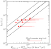 |
Fig. 2. Infrared luminosities measured for 11 ALPINE FIR continuum-detected nonmerger galaxies (Béthermin et al. 2020) as a function of their CO(1–0) luminosities inferred from the [C II] molecular gas masses and a range of CO-to-H2 conversion factors (dotted red lines) from the Milky Way value of 4.36 M⊙ (K km s−1 pc2)−1 (on the left) to the starburst value of 1 M⊙ (K km s−1 pc2)−1 (on the right). The solid black line shows the best fit of Dessauges-Zavadsky et al. (2015) of the empirical LIR– |

3.2.2. Dust continuum molecular gas masses
At long wavelengths in the Rayleigh-Jeans tail regime (λrest ≳ 250 μm), the thermal dust emission is optically thin and the observed flux density is directly dependent on the mass of dust, the dust opacity coefficient, and the mean temperature of dust contributing to the emission at these wavelengths (Scoville et al. 2016). By assuming a dust-to-gas mass ratio and that the molecular gas dominates the overall gas budget (the atomic and ionized gas content being negligible), we can then recover the molecular gas mass from the derived dust mass. The rest-frame 850 μm luminosity (L850 μm) was found to exhibit a tight correlation with the ISM molecular gas mass and is now frequently used as a molecular gas tracer (Scoville et al. 2014, 2016, 2017; Hughes et al. 2017b; Privon et al. 2018; Kaasinen et al. 2019). The difficulty remains in deriving L850 μm from a single-band FIR continuum measurement, since this requires us to assume a dust opacity coefficient and a mean dust temperature, or to know the FIR SED characteristic of the studied galaxies.
Béthermin et al. (2020) constructed the mean stacked FIR SEDs specific to ALPINE galaxy analogues following the same prescriptions as in Béthermin et al. (2015), but using the more recent COSMOS catalogue of Davidzon et al. (2017) and deep SCUBA2 data at 850 μm from Casey et al. (2013). Moreover, the targets to be stacked were selected with properties analogous to the ones of the ALPINE galaxies: SFR ≳ 10 M⊙ yr−1, and redshift bins of 4 < z < 5 and 5 < z < 6. The resulting SEDs are best fit by the Béthermin et al. (2017) SED template, but both the Schreiber et al. (2018) SED template and a modified blackbody (MBB) with dust opacity spectral index fixed to β = 1.8 and luminosity-weighted dust temperature of 41 ± 1 K at z < 5 and 43 ± 5 K at z > 5 provide a good fit (χ2 < 4 for 4 degrees of freedom; see Fig. 9 in Béthermin et al. 2020).
We adopt the Béthermin et al. (2017) FIR SED template to estimate L850 μm of the 11 ALPINE nonmerger galaxies with FIR continuum detections by scaling the measured monochromatic rest-frame 158 μm luminosity by the ratio between the SED-predicted luminosities at 850 μm and 158 μm. Subsequently, using the calibration of Scoville et al. (2016)3,
 (2)
(2)
we derive the molecular gas masses from the extrapolated rest-frame 850 μm luminosities. These values, although reliant on multiple assumptions (e.g., SED template, constant dust-to-gas mass ratio of 1:100), are independent measurements to be compared with  inferred from the [C II] luminosity. The comparison is shown in Fig. 3. Within 1 − 2σ uncertainty of 0.3 − 0.6 dex, we find an agreement between these two measurements, although there is some trend for a systematic overestimation of
  with respect to
  by 0.3 dex, on average. A similar offset is observed for the Schreiber et al. (2018) SED template and the MBB. On the other hand, when considering the calibration of Groves et al. (2015, Table 5), obtained for local galaxies with log(Mstars/M⊙) > 9, between monochromatic luminosity in the Herschel PACS 160 μm band and gas mass, which relies on far fewer assumptions, we find only a marginal overestimation by 0.1 dex of
  relative to these gas mass estimates.
 |
Fig. 3. Comparison of molecular gas masses of the 11 ALPINE FIR continuum-detected nonmerger galaxies as derived from the [C II] luminosity (Eq. (1)) and the rest-frame 850 μm luminosity (Eq. (2)). The monochromatic rest-frame 850 μm luminosity is extrapolated from the measured rest-frame 158 μm luminosity by assuming either the FIR SED template of Béthermin et al. (2017) (filled circles), or the MBB curve with β = 1.8 and Tdust = 25 K as adopted by Scoville et al. (2016, 2017) (filled stars). The open squares show the molecular gas masses derived directly from the measured rest-frame 158 μm luminosity using the calibration of Groves et al. (2015), obtained for local galaxies, between Herschel PACS 160 μm monochromatic luminosity and gas mass. The dotted line is the one-to-one relation. Overall, there is good agreement between |

The observed  overestimation with respect to
  may be attributed to three possible effects. First, it points to potential contributions from the neutral atomic and ionized phases to the measured [C II] emission, in addition to the molecular gas phase. Second, it suggests that the calibration of Scoville et al. (2016) may not be valid for the ALPINE galaxies at z ≳ 4.5. It should be pointed out that Scoville et al. (2014, 2016) and Kaasinen et al. (2019) state that the L850 μm–
 relation only holds for massive SFGs with Mstars > 1010.3 M⊙ and breaks down for galaxies of lower stellar mass (see also Dessauges-Zavadsky et al. 2015), partly because of the assumed constant dust-to-gas mass ratio of 1:100. This is also shown by the simulation-based studies of Liang et al. (2018) and Privon et al. (2018). The ALPINE galaxies with a median stellar mass of 109.7 M⊙ enter the lower mass regime, and are, in addition, found to be deficient in dust-obscured star formation activity with respect to lower redshift SFGs (Fudamoto et al. 2020). We may therefore expect a lower dust-to-gas mass ratio (∝α850 μm in Eq. (2)). Indeed, to reconcile
  with
with  , α850 μm would need to be lower by a factor of approximately two. Third, the observed
  overestimate supports the idea that the SED in the Rayleigh-Jeans tail out to 850 μm rest-frame could be dominated by a cold component because we get comparable
  to
to  (Fig. 3) when
  values are obtained via Eq. (2), this time with 850 μm luminosities extrapolated from the measured 158 μm luminosities by assuming a MBB SED parametrization with the cold mass-weighted dust temperature of Tdust = 25 K and β = 1.8, similarly to Scoville et al. (2016, 2017).
3.2.3. Dynamical masses
As described in Le Fèvre et al. (2020), 2/3 of the ALPINE [C II]-detected galaxies are moderately spatially resolved. For a subset of 18 nonmerger galaxies with high-S/N (≳5) [C II] detections, Fujimoto et al. (2020) derived their [C II] sizes by performing exponential-disk profile fits in the visibility plane with UVMULTIFIT (Martí-Vidal et al. 2014). The circularized effective radii (re), defined as the square root of the product of the effective major and minor axes, are adopted as size measurements and are listed in Table 1 of Fujimoto et al. (2020). For the ALPINE galaxies with size measurements, we can derive their dynamical masses under the assumption that the gas potential structure of ALPINE galaxies arises in a virialised spherical system of radius equal to the measured circularized effective radius and with the one-dimensional velocity dispersion (σCII) inferred from the full width at half maximum ( ) of the [C II] line corrected for final channel spacing4:
 (3)
(3)
following Eq. (10) in Bothwell et al. (2013). These virialized, spherical-geometry dynamical masses are 0.13 dex larger than the dynamical masses we would obtain if we assumed a disk-like gas potential distribution for the same source size, the same  , and a mean inclination angle (i) of the source of ⟨sin i⟩=π/4 (Law et al. 2009; Wang et al. 2013; Capak et al. 2015). However, the virial masses confer the advantage that the supplementary uncertainty on the source orientation required in the computation of the dynamical masses for disk geometry does not need to be added. For 5 out of the 9 ALPINE galaxies classified as rotation-dominated systems (Le Fèvre et al. 2020), we obtained robust [C II] minor-to-major-axis ratio measurements (Fujimoto et al. 2020), which enable us to constrain their disk inclination angles as i = cos−1(minor/major). For these 5 galaxies, we also compute dynamical masses for the disk-like gas potential distribution:
 (4)
(4)
where the circular velocity of the gaseous disk is υcir = 1.763σCII/sin(i). The corresponding dynamical masses are randomly scattered by up to ±0.25 dex from virial masses.
Since the relative contribution of dark-matter in the internal regions of galaxies (at < (1 − 2)re) is expected to be low (Barnabè et al. 2012 report a dark-matter fraction within 2.2re of at most  ), the dynamical mass may be assumed to reflect the total baryonic mass, which can be used to obtain an estimate of Mmolgas after subtracting Mstars. Out of the 18 ALPINE nonmerger galaxies with size measurements, for one galaxy5 the virial mass is smaller than its Mstars. For the remaining 17 ALPINE galaxies, we can cross-match the molecular gas masses obtained from their dynamical and stellar masses with the gas masses inferred from their [C II] luminosities. For 12 ALPINE galaxies we consider the virial masses, and for the 5 ALPINE galaxies classified as rotation-dominated we consider the dynamical masses derived for a disk-like gas potential. As shown in Fig. 4, there is good agreement within the 1σ uncertainty of 0.3 dex between these respective molecular gas mass estimates, except for two outliers (which do not show any systematic trend). We may see the good one-to-one relationship between the two molecular gas mass estimates not only as a corroboration of the Zanella et al. (2018)LCII–
 relation, but also as an independent calibration, valid for MS SFGs at 4.4 < z < 5.9, between LCII and the total gas mass (including all the molecular, atomic, and ionized phases), as inferred from the baryonic content traced by the dynamical mass.
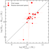 |
Fig. 4. Comparison of molecular gas masses of ALPINE nonmerger galaxies as derived from the [C II] luminosity (Eq. (1)) and the dynamical mass after subtracting Mstars (the relative contribution of dark-matter is assumed to be negligible). The dynamical masses, accessible only for the ALPINE galaxies with available [C II] size measurements (Fujimoto et al. 2020), are computed using the virial mass definition (Eq. (3); filled circles), except for 5 objects classified as rotation-dominated (Le Fèvre et al. 2020) for which we consider the disk-like gas potential distribution (Eq. (4); crosses). The dotted line is the one-to-one relation. There is good agreement between |

4. Comparison sample
Tremendous observational efforts have been dedicated to determining the molecular gas content of galaxies from the present time to high redshift using either the CO emission or the FIR dust continuum as molecular gas mass tracers. These tracers have their respective strengths and weaknesses (see Bolatto et al. 2013; Genzel et al. 2015; Scoville et al. 2016; Tacconi et al. 2018). While the former is the most commonly used and well-calibrated tracer in the local Universe, the latter, which usually relies on a single-band continuum measurement preferably in the Rayleigh-Jeans tail of the FIR SED, is particularly inexpensive in terms of ALMA observing time. Here we propose to compare the ALPINE  with a compilation of local to high-redshift MS SFGs with molecular gas masses derived from CO luminosity measurements reported in the literature.
We build up the database of CO-detected MS SFGs starting from the exhaustive compilation of CO luminosity measurements in MS SFGs at z > 1 presented in Dessauges-Zavadsky et al. (2015, 2017). We extend this compilation with published CO luminosity measurements at z > 1 from 20156 onwards by Seko et al. (2016), Papovich et al. (2016), González-López et al. (2017), Magdis et al. (2017), Valentino et al. (2018), Gowardhan et al. (2019), Kaasinen et al. (2019), Molina et al. (2019), Aravena et al. (2019), Bourne et al. (2019), Pavesi et al. (2019), and Cassata et al. (2020). Furthermore, we include the release of the NOEMA PHIBSS2 legacy survey at 0.5 < z < 2.5, described in Tacconi et al. (2018) and Freundlich et al. (2019). We adopt the MS parametrization from Speagle et al. (2014, Eq. (28)), similarly to what was done for PHIBSS2, and retain only SFGs lying within the MS dispersion of ΔMS = log(SFR/SFRMS) = ± 0.3 dex. Our updated compilation comprises a total of 101 CO luminosity measurements for MS SFGs at 1 < z < 3.7 and with Mstars = 109.5 − 1011.7 M⊙, plus the CO detection at z = 5.65 from Pavesi et al. (2019); however, this compilation is still under-sampled at high redshift (z > 2.5) and at the low-Mstars end (Mstars < 1010 M⊙). The compilation of Dessauges-Zavadsky et al. (2015) also contained CO(1–0) measurements for a non-exhaustive number of local spiral galaxies and MS SFGs at z < 1. We now add the CO(1–0) measurements from the final xCOLD GASS survey at 0.01 < z < 0.05 performed with the IRAM 30 m telescope (Saintonge et al. 2016, 2017), which now extends to lower Mstars than in previous samples, namely log(Mstars/M⊙) = 9 − 10.
At z > 0.5, the CO(1–0) transition is often replaced by a high-J CO transition with J = 2 to 5, which requires the calibration of temperature and density from the CO spectral line energy distribution (CO SLED) to access the CO luminosity correction factor  . CO SLED observations in MS SFGs at z ∼ 1 − 3.7 converge on r2, 1 = 0.81 ± 0.15, r3, 1 = 0.57 ± 0.11, r4, 1 = 0.33 ± 0.06, and r5, 1 = 0.23 ± 0.04 (Daddi et al. 2015; Dessauges-Zavadsky et al. 2015, 2019; Cassata et al. 2020). In order to have a homogeneous comparison sample, we adopt these CO luminosity correction factors to all CO J → J − 1 luminosity measurements in our compilation, and we derive the molecular gas masses,
  , assuming the same CO-to-H2 metallicity-dependent conversion function:
 (5)
(5)
which corresponds to the geometrical mean of the metallicity-dependent conversion functions of Bolatto et al. (2013) and Genzel et al. (2012) following Eq. (2) in Tacconi et al. (2018)7. We adopt the Milky Way CO-to-H2 conversion factor of Strong & Mattox (1996), αCO, MW = 4.36 M⊙ (K km s−1 pc2)−1, which includes the correction factor of 1.36 for helium. To estimate the metallicities of the CO-detected SFGs when direct metallicity measurements are not available, we use the redshift-dependent mass–metallicity relation defined by Genzel et al. (2015)8 and calibrated to the Pettini & Pagel (2004) metallicity scale and the solar abundance of 12 + log(O/H)⊙ = 8.67 (Asplund et al. 2004):
 (6)
(6)
with a = 8.74 and b = 10.4 + 4.46log(1 + z)−1.78(log(1 + z))2. As discussed in Dessauges-Zavadsky et al. (2017),  increases with redshift for any given Mstars, and increases with decreasing Mstars at any given redshift. As a result,
  might be particularly uncertain at high redshift (z ≳ 3) and for small Mstars (Mstars ≲ 1010 M⊙) because of the more poorly constrained mass–metallicity relation in this range of physical parameters.
Finally, to check whether or not our compilation of high-redshift SFGs at 0.1 < z < 3.7 with molecular gas masses derived from CO luminosity measurements is representative of MS SFGs at these redshifts, we consider the mean Mmolgas obtained by Béthermin et al. (2015) from their stacking analysis of the IR-to-millimeter emission of MS SFGs, with an average Mstars of ∼1010.8 M⊙, blindly selected in the COSMOS field between z = 0.25 and z = 4. For a coherent comparison, we rescale the molecular gas masses of Béthermin et al. (2015) to the mass–metallicity relation used in the CO compilation (Eq. (6)). Nevertheless, we keep the metallicity correction of 0.3 × (1.7 − z) dex that these latter authors applied at z > 1.7 and which becomes significant for galaxies beyond z > 2.5. We find that the respective molecular gas depletion timescales and gas fractions globally agree, supporting the idea that the sample of CO-detected SFGs is unbiased, except maybe in the redshift bin of 1 < z < 1.5 where the CO-measured molecular gas masses tend to be higher than the Béthermin et al. (2015) FIR SED stack results (see Fig. 6, left panel and Fig. 8, top panel).
Recently, Liu et al. (2019b) published Mmolgas measurements for about 700 galaxies at 0.3 < z < 6 extracted on an automated prior-based and blind-based ALMA Archive mining in the COSMOS field (hereafter A3COSMOS, with spectroscopic redshifts available for 36% of the sample Liu et al. 2019a). The molecular gas masses were derived from single-band FIR continuum and multi-wavelength FIR SEDs. However, the A3COSMOS galaxies are mostly probing the high Mstars domain of MS SFGs at z > 1 with Mstars ∼ 1011 − 1012 M⊙. Therefore, on average, they are 10 − 100 times more massive than the ALPINE [C II]-detected galaxies that have a median Mstars of ∼109.7 M⊙ (and a mean of ∼1010 M⊙). Consequently, in terms of the respective Mstars distributions shown in Fig. 5, our compilation of CO-detected MS galaxies at z > 1 represents a better comparison sample for the ALPINE galaxies, despite the fact that in the redshift range of ALPINE galaxies (z = 4.4 − 5.9) one single CO detection is included, compared to 24 Mmolgas measurements for MS SFGs in the A3COSMOS sample. With a median Mstars of ∼1010.9 M⊙ (and a mean of ∼1011 M⊙), the CO-detected SFGs globally have adequate masses at 1 < z < 3.7 to plausibly be the descendants of the ALPINE galaxies according to the multi-epoch abundance-matching simulations (Behroozi et al. 2013, 2019; Moster et al. 2013, 2018), as discussed in Sect. 5.4.
 |
Fig. 5. Distribution of stellar masses of the 44 ALPINE [C II]-detected nonmerger galaxies at z = 4.4 − 5.9 (red histogram) and the comparison sample of 101 CO-detected MS SFGs at 1 < z < 3.7 compiled from the literature (gray histogram). The solid and dashed lines correspond, respectively, to the medians and means of the two distributions. The black thick lines show the range and the mean of Mstars of the A3COSMOS galaxies at 1 < z < 6 (Liu et al. 2019b). Clearly, the ALPINE sample probes a much lower Mstars range than previous galaxy samples with molecular gas mass measurements obtained mostly at lower redshift. |
5. Analysis and discussion
5.1. Link to the Kennicutt-Schmidt relation
As discussed in Sect. 3.1, the origin of the [C II] emission is complex, because different gas phases (ionized, neutral, and molecular) contribute to it, and therefore identifying which one dominates the observed flux is difficult. This is probably why two different empirical relations, between LCII and SFR (as observed in the Milky Way, nearby galaxies, and SFGs up to z ∼ 2; see, e.g., Pineda et al. 2014; Herrera-Camus et al. 2015; De Looze et al. 2011, 2014), and between LCII and Mmolgas (discussed in Sect. 3.1), were established and reported in the literature. Fundamental arguments nevertheless support a direct physical connection between LCII and SFR. Indeed, far-UV (FUV) photons produced by young, massive stars heat the gas via the photoelectric effect on dust grains (Hollenbach & Tielens 1999). The resulting ejected photoelectrons heat the gas, and then neutral collisions excite the C+ ions and the gas cools via emission of [C II] photons. Thus, if the gas is in thermal balance and the [C II] line is the main cooling channel, the [C II] luminosity is a tracer of the total energy deposited into the gas by the star formation activity (SFR ∝ LFUV ∝ ϵphLCII, where ϵph is the photoelectric heating efficiency). As a result, the [C II] luminosity depends on the mutual interaction of SFR (providing FUV photons necessary for the heating) with the amount of emitting material (neutral/molecular gas) available in a galaxy. Consequently, the link between LCII and Mmolgas is likely a by-product of the KS star-formation law that connects SFR to Mmolgas (Kennicutt 1998b). Ferrara et al. (2019), for instance, find evidence in their analytical model that the KS relation is influencing the [C II] luminosity. In particular, these latter authors find that upward deviations from the KS relation cause a “paucity” of gas at fixed SFR, and can thus produce a decrease in LCII at a given SFR.
Schaerer et al. (2020) studied the LCII–SFR relation for the ALPINE MS SFGs and find that the local relation of De Looze et al. (2014) still holds (possibly with very little evolution) at 4.4 < z < 5.9. Together with the LCII–Mmolgas relation of Zanella et al. (2018), which also seems to hold within a ∼0.3 dex uncertainty as shown by the good match between the molecular gas masses inferred from the [C II] luminosity and three independent gas mass tracers (see Sect. 3.2), we suggest that no significant deviation from the KS law established for nearby SFGs is expected for our high-redshift sample. Further work on the actual location of the ALPINE galaxies with respect to the KS relation will be presented in the future (paper in prep.).
In what follows, we assume that we can adopt the [C II]-derived gas masses for the ALPINE galaxies to study the evolution of the molecular gas content of MS SFGs up to z ∼ 6. We emphasize that if instead we choose another of the tested molecular gas mass tracers, we would obtain similar conclusions. This is particularly important in the derivation of the molecular gas depletion timescales defined as tdepl = Mmolgas/SFR, since the use of  in tdepl measurements must be done with caution given that, following the above discussion,
  already indirectly rely on the assumption of the SFR–Mmolgas KS scaling relation.
5.2. Molecular gas depletion timescale
The molecular gas depletion timescale (or gas-consumption timescale) describes how long each galaxy may sustain star formation at the measured rate before running out of molecular gas fuel under the assumption that the gas reservoir is not replenished. Since the earliest CO luminosity measurements in high-redshift MS SFGs, evidence has been found for shorter tdepl at high redshift such that tdepl ∼ 1 − 2 Gyr observed at z = 0 (e.g., Bigiel et al. 2008; Leroy et al. 2013; Saintonge et al. 2017) drops by a factor of about two at z ∼ 2.5 (e.g., Tacconi et al. 2013, 2018, 2020; Saintonge et al. 2013; Genzel et al. 2015; Béthermin et al. 2015; Dessauges-Zavadsky et al. 2015, 2017; Schinnerer et al. 2016; Scoville et al. 2017; Liu et al. 2019b), following the (1 + z)−0.62 ± 0.13 decline as measured by Tacconi et al. (2018). Shorter tdepl correspond to higher star formation efficiencies (SFE = 1/tdepl) that are taking place in high-redshift galaxies, efficient enough to exhaust similar and even larger gas reservoirs over a shorter timescale than in nearby MS SFGs. The so-far inferred tdepl evolution with redshift up to z ∼ 3.5 nevertheless appears much shallower than tdepl ∼ (1 + z)−1.5 (see Fig. 6, left panel), which is predicted by semi-analytical and cosmological simulations developed in the framework of the bathtub model (e.g., Davé et al. 2011, 2012; Genel et al. 2014; Lagos et al. 2015). This suggests that distant galaxies either intrinsically do not have such high SFE, or are more gas-rich than predicted, or outflows, if highly mass loaded, contribute to reduce the gas.
 |
Fig. 6. Molecular gas depletion timescales plotted for the ALPINE nonmerger galaxies distributed in two redshift bins of 4.4 < z < 4.6 and 5.1 < z < 5.9 (red circles; encircled red circles mark the ALPINE galaxies detected in FIR dust continuum; crossed red circles mark the ALPINE galaxies with dynamical mass measurements; and light-red arrows correspond to 3σ upper limits) and for our compilation of CO-detected MS SFGs from the literature color-coded in six redshift bins of z = 0 (pink crosses), 0 < z < 0.1 (yellow pluses), 0.1 < z < 1 (orange stars), 1 < z < 1.5 (violet open pentagons), 1.5 < z < 2.5 (green squares), and 2.5 < z < 3.7 (blue triangles, plus the Pavesi et al. 2019 object at z = 5.65). Left panel: molecular gas depletion timescales shown as a function of redshift. The respective means, errors on the means, and standard deviations per redshift bin are indicated by the large black/gray crosses. The light-gray shaded area corresponds to the depletion timescales obtained by Béthermin et al. (2015) from FIR SED stacks. The tdepl means per redshift bin follow a decrease out to z ∼ 6, but much shallower than the (1 + z)−1.5 decline predicted in the framework of the bathtub model (dotted line). Middle panel: molecular depletion timescales shown as a function of specific star formation rate. A strong anti-correlation between tdepl and sSFR is observed at z = 0 (yellow solid line from Saintonge et al. 2011) and at high redshift. The displacement along the sSFR-axis for galaxies at higher redshift is compatible with the sSFR evolution with redshift (violet dashed line at z = 1, green dashed-dotted line at z = 2, and red dotted line at z = 5, as computed using the sSFR(z) parametrization from Speagle et al. 2014, Eq. (28)). Right panel: molecular depletion timescales restricted to z = 1 − 5.9 SFGs and shown as a function of stellar mass. No correlation between tdepl and Mstars is observed. |
The ALPINE sample enables us, for the first time, to explore the tdepl evolution beyond z ≳ 4.5 for a statistically significant number of MS SFGs with a median Mstars of 109.7 M⊙. The measured tdepl means, errors, and standard deviations in two redshift bins of 4.4 < z < 4.6 and 5.1 < z < 5.9 are listed in Table 1. We provide both the means obtained when considering only the 44 [C II]-detected galaxies and when also taking into account the secure 3σ upper limits of the 43 galaxies undetected in [C II] (see Sect. 2). The latter means are computed using the survival analysis (with routines described in Isobe et al. 1986). In particular, we use the Kaplan-Meier estimator, an unbiased nonparametric maximum-likelihood estimator that determines the characteristic of a parent population with no assumption on the distribution of the parent population from which the censored sample is drawn. The respective tdepl means with or without limits differ by about a factor of two. Finally, in Table 1 we also provide an independent tdepl mean (and standard deviation) computed by considering only molecular gas masses inferred from dynamical masses (see Sect. 3.2.3). We find good agreement between the respective tdepl means measured for the ALPINE sub-sample of 17 galaxies with dynamical mass measurements. This agreement supports the conclusion that the [C II]-derived tdepl values intrinsically show a smooth tdepl redshift evolution (see below), which does not result from an incorrect trend of the KS law conservation in the ALPINE MS SFGs at 4.4 < z < 5.9 discussed in Sect. 5.1. Within the error bars, the corresponding tdepl means also match the tdepl mean of the whole ALPINE [C II]-detected nonmerger sample.
ALPINE molecular gas depletion timescales and molecular gas fractions in two redshift bins.
In the left panel of Fig. 6 we show the molecular gas depletion timescale as a function of redshift for the ALPINE [C II]-detected nonmerger galaxies (red circles) and [C II]-nondetected galaxies (light-red arrows) distributed in two redshift bins of 4.4 < z < 4.6 and 5.1 < z < 5.9, and for our compilation of CO-detected MS SFGs from the literature separated in six redshift bins of z = 0, 0 < z < 0.1, 0.1 < z < 1, 1 < z < 1.5, 1.5 < z < 2.5, and 2.5 < z < 3.7. These bins were chosen in such a way that the three bins between z = 0.1 and z = 2.5 contain a comparable number of galaxies (∼40). We then compute the respective means, errors on the means, and standard deviations per redshift bin (large black/gray crosses). We show the ALPINE means obtained for the 44 [C II] detections and given in Table 1. We also overplot the depletion timescales obtained by Béthermin et al. (2015) from FIR SED stacks (light-gray shaded area). We observe a continuous decline of tdepl from z = 0 to z = 5.9. The decline follows a power law with a slope that is clearly shallower than (1 + z)−1.5 (dotted line), as this latter would imply tdepl = 6.0 × 10⁷ yr at z = 5.5 when fixing the zero-point at z = 0 to 1 Gyr (Saintonge et al. 2017). This predicted tdepl value is comparable to the smallest ALPINE tdepl measurement, but is almost one order of magnitude shorter than the mean tdepl of (4.6 ± 0.8) × 108 yr of the ALPINE [C II]-detected nonmerger galaxies in the redshift bin of 5.1 < z < 5.9. For the ALPINE galaxies undetected in the FIR continuum emission, even if we add to their measured SFRUV the possible SFRIR contribution estimated using the ALPINE IRX–β relation obtained from stacking (Fudamoto et al. 2020) as discussed in Sect. 2, the resulting mean tdepl of ∼3.8 × 10⁸ yr over 4.4 < z < 5.9 is still too long compared to the (1 + z)−1.5 decline. When taking into account the secure 3σ upper limits of the ALPINE galaxies undetected in [C II], the mean tdepl drops to (2.3 ± 0.4) × 108 yr in the redshift bin of 5.1 < z < 5.9 (see Table 1). This drop suggests a steeper tdepl decrease with redshift than shown by [C II] detections, but the corresponding mean tdepl value is still a factor of approximately four longer than for the predicted one. Consequently, on average, MS SFGs at z ≳ 4.5 are not considerably more efficient in forming stars than MS SFGs at z ∼ 2 − 3, as also supported by the low SFE obtained by Pavesi et al. (2019) from the CO(2–1) molecular gas mass measurement in a MS SFG at z = 5.65 (see the blue triangle at z = 5.65 in the left panel of Fig. 6).
There is significant scatter (larger than 1 dex) among the tdepl measurements in all redshift bins, even though we only consider MS galaxies with ΔMS = ±0.3 dex around the MS parametrization of Speagle et al. (2014). This scatter at a fixed redshift is believed to be a product of the multi-functional dependence of tdepl on many physical parameters, such as the offset from the MS, the star formation rate, the stellar mass, and possibly the environment (e.g., Dessauges-Zavadsky et al. 2015; Scoville et al. 2017; Noble et al. 2017; Silverman et al. 2018; Tacconi et al. 2018; Tadaki et al. 2019; Liu et al. 2019b). Given the strong anti-correlation found between tdepl and the offset from the MS (Genzel et al. 2015; Dessauges-Zavadsky et al. 2015; Tacconi et al. 2018), we still expect tdepl variations for galaxies on the MS while in their evolutionary process they are transiting up and down across the MS band (e.g., Sargent et al. 2014; Tacchella et al. 2016). The previously reported anti-correlation between tdepl and sSFR (Saintonge et al. 2011; Dessauges-Zavadsky et al. 2015) is also further supported by our galaxies at z = 4.4 − 5.9 (Fig. 6, middle panel). This highlights comparable timescales for gas consumption and stellar mass formation. We find a Spearman rank coefficient of −0.49 and p-value of 4.5 × 10⁻¹⁰ for the dependence of tdepl on sSFR when considering the MS SFGs at z ∼ 1 − 5.9. The observed offset of ALPINE galaxies with respect to the tdepl–sSFR relation of MS SFGs at z = 0 and to a smaller extent to the relations at z ∼ 1 and z ∼ 2 is compatible with the displacement of the z = 0 relation along the sSFR-axis by factors derived from the sSFR evolution with redshift of MS SFGs out to z ∼ 5 (Speagle et al. 2014). Nevertheless, a less steep sSFR redshift evolution toward z ∼ 5 than parametrized by Speagle et al. (2014) is suggested by the ALPINE sample, in line with the sSFR(z) results of Khusanova et al. (2020a). On the other hand, with tdepl measurements achieved down to Mstars ∼ 108.4 M⊙ for the ALPINE galaxies, we confirm that for MS SFGs at z ∼ 1 − 5.9 the tdepl dependence on Mstars, if any, must be weak as shown in Fig. 6 (right panel). This further supports the idea that the linear KS relation established for local galaxies (Kennicutt 1998b) might hold up to z ∼ 5.9 for MS SFGs.
For their respective compilations of galaxies with Mmolgas measurements, Scoville et al. (2017), Tacconi et al. (2018), and Liu et al. (2019b) performed a multi-functional fitting to simultaneously quantify the underlying dependency of tdepl as products of power laws in redshift, Mstars, and offset from the MS (as well as optical size in the case of Tacconi et al. 2018, who ultimately found a negligible tdepl dependence on size). These three groups of authors used slightly different criteria in their fitting procedures, but assumed the same MS parametrization from Speagle et al. (2014, Eq. (28))9. Their respective best fits yield different tdepl functional forms, which are compared in Liu et al. (2019b). While the Tacconi et al. (2018)tdepl function was fitted with data covering only redshifts of z ∼ 0 − 3, the Liu et al. (2019b) function accounts for data at z > 3, albeit restricted to MS SFGs with high Mstars (Mstars ∼ 1011 M⊙). All the three fitted functions lack constraints for MS low stellar mass (Mstars ≲ 1010 M⊙) SFGs at z > 3. These SFGs are particularly important because, as shown by Liu et al. (2019b), the largest differences between the three fitted tdepl functions are observed for MS SFGs at z > 4 with Mstars < 1010 M⊙. The ALPINE galaxies are precisely characterized by these physical properties and can therefore bring decisive constraints on the tdepl function.
The top panels of Fig. 7 show, similarly to Liu et al. (2019b), the molecular gas depletion timescale as a function of redshift as predicted by the three tdepl best-fit functions for MS galaxies with ΔMS ranging from −0.3 dex to +0.3 dex and stellar masses in two bins of  and
and  . To compare the observations with the plotted best-fit functions, we bin the ALPINE galaxies in two redshift intervals of 4.4 < z < 4.6 and 5.1 < z < 5.9 (red boxes), and the CO-detected MS SFGs from our compilation (Sect. 4) in three redshift intervals of 1 < z < 1.5, 1.5 < z < 2.5, and 2.5 < z < 3.7 (gray boxes). The blue boxes represent MS SFGs at 0 < z < 1 from A3COSMOS in Δz = 0.3 bins (Liu et al. 2019b). The ALPINE galaxies exclude the tdepl best-fit function of Liu et al. (2019b) at z ≳ 4.5 in the two Mstars bins, but already in the redshift bin of 2.5 < z < 3.7 we observe a deviation from this function in the
  bin. On the other hand, both the Scoville et al. (2017) and Tacconi et al. (2018)tdepl functions agree with the ALPINE observations, even if we consider the possible SFRIR contribution for the ALPINE galaxies undetected in the FIR dust continuum (see Sect. 2), which would lower the plotted tdepl means by a factor of 1.5 in the redshift bin of 4.4 < z < 4.6 and less in the higher redshift bin. The discrepancy of the Liu et al. (2019b) best-fit function with the other two functions results from the strong anti-correlation that these latter authors find between tdepl and Mstars. This dependence of tdepl on Mstars is too strong for SFGs with Mstars < 1010.5 M⊙ at z ≳ 3, but seems to be correct at the high stellar mass end of Mstars ≳ 1011 M⊙ where both the Scoville et al. (2017) and Tacconi et al. (2018) functions overestimate the tdepl measurements at z ≳ 3 (see Fig. 12 in Liu et al. 2019b). We defer a refitting of the functional form of tdepl by including ALPINE galaxies in order to determine the scaling relation of tdepl over a more complete Mstars and redshift range to a future paper.
 |
Fig. 7. Redshift evolution of the molecular gas depletion timescale (top panels) and the molecular gas mass to stellar mass ratio (bottom panels) of MS galaxies ( |

5.3. Molecular gas fraction
In the top panel of Fig. 8 we show the molecular gas fraction, defined as fmolgas = Mmolgas/(Mmolgas + Mstars), as a function of redshift for the ALPINE [C II]-detected nonmerger galaxies (red circles) and [C II]-nondetected galaxies (light-red arrows) in two redshift bins of 4.4 < z < 4.6 and 5.1 < z < 5.9, and for our compilation of CO-detected MS SFGs from the literature separated in the same six redshift bins as in Fig. 6. We then compute the respective means, errors on the means, and standard deviations per redshift bin (large black/gray crosses). We show the ALPINE means obtained for the 44 [C II] detections (see Table 1). We also overplot the Béthermin et al. (2015) FIR SED stacks (light-gray shaded area). We observe a steep rise of fmolgas from z = 0 to z ∼ 3.7, in agreement with what has been previously reported (e.g., Dessauges-Zavadsky et al. 2017; Scoville et al. 2017; Tacconi et al. 2018, 2020). With the ALPINE sample, we probe, for the first time, the fmolgas evolution beyond z ≳ 4.5 of MS SFGs with a low median Mstars of 109.7 M⊙. Within the 1σ dispersion on the fmolgas means in the two redshift bins, we observe a flattening of fmolgas that reaches a mean value of 63%±3% over z = 4.4 − 5.9. The observed flattening does not result from the assumptions that are considered to translate [C II] luminosities into molecular gas masses, since both 4.4 < z < 4.6 and 5.1 < z < 5.9 bins are subject to those assumptions in the same way. When applying the survival analysis to take into account the secure 3σ upper limits of the ALPINE galaxies undetected in [C II] (see Sect. 5.2), the fmolgas means in the 4.4 < z < 4.6 and 5.1 < z < 5.9 bins drop to 46%±5% (Table 1). This strengthens the fmolgas flattening toward high redshift, which is an important result, consistent with the evolutionary trend of a constant sSFR beyond z ≳ 4 obtained by several studies (e.g., Tasca et al. 2015; Khusanova et al. 2020b), including sSFR derived from the dust-obscured SFR measured in the ALPINE galaxies by stacking the FIR dust continuum maps in the redshift bins of 4.4 < z < 4.6 and 5.1 < z < 5.9 (Khusanova et al. 2020a). The finding that fmolgas and sSFR merely have a similar evolution with redshift is not a surprise, since fmolgas can be expressed as a function of tdepl and sSFR (Tacconi et al. 2013):
 (7)
(7)
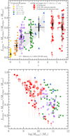 |
Fig. 8. Molecular gas fractions plotted for the same ALPINE galaxies (red circles) and CO-detected MS SFGs with the same color coding per redshift bin as in Fig. 6. Top panel: molecular gas fractions shown as a function of redshift. The respective means, errors on the means, and standard deviations per redshift bin are indicated by the large black/gray crosses. The light-gray shaded area corresponds to the molecular gas fractions obtained by Béthermin et al. (2015) from FIR SED stacks. The fmolgas means per redshift bin show a steep increase from z = 0 to z ∼ 3.7, followed by a flattening toward higher redshift within the 1σ dispersion on the means. Bottom panel: molecular gas fractions restricted to z ∼ 1 − 5.9 SFGs and shown as a function of stellar mass. A strong dependence of fmolgas on Mstars is observed for CO-detected high-redshift galaxies and the ALPINE galaxies as well. |
Consequently, the fmolgas redshift evolution depends on the redshift evolution of both tdepl and sSFR. In the case of a weak change of tdepl with redshift for MS SFGs, on average, which is what we observe in Fig. 6 (left panel), we globally have fmolgas(z)∝sSFR(z).
In the framework of the bathtub model, the fmolgas evolution with redshift reflects an interplay between cosmic inflow (supply of fresh gas onto galaxies) and gas consumption rates, modulo outflows. The mass accretion rate was shown to scale as (1 + z)2.25 (Dekel et al. 2009), and therefore the gas supply rate drops faster with time than the gas consumption rate (see Sect. 5.2). This explains why galaxies at sufficiently high redshift begin to be gas-rich, but then fmolgas drops as the gas consumption rate catches up. The phase during which galaxies have an excess of gas, and hence are in nonequilibrium, will also depend on feedback, because outflows, by ejecting the gas out of galaxies, reduce the amount of gas that needs to be processed into stars and help to establish the equilibrium earlier on. A quick look at the fmolgas observations supports a gas excess until at most z ∼ 3 (Fig. 8, top panel). This is much shorter in cosmic time than predicted by the cosmological simulations of Lagos et al. (2015), who report a drop of fmolgas only several gigayears later, by z ∼ 1. Given the shallow tdepl evolution with redshift, outflows must play an important role in blowing out part of the infalling gas at z ≳ 3. This is supported by signatures of star-formation-driven outflows in stacks of [C II] spectra and [C II] moment-zero maps, and in stacks of rest-frame UV spectra of the ALPINE higher SFR (≳25 M⊙ yr−1) galaxies (Ginolfi et al. 2020c; Faisst et al. 2020), but also observed in a few individual ALPINE objects with [C II] halos (Fujimoto et al. 2020; Ginolfi et al. 2020b). Observational evidence of star-formation-driven outflows in SFGs at z ≲ 5 − 6 was also reported in other studies (e.g., Sugahara et al. 2019; Rubin et al. 2014; Talia et al. 2017).
While we observe an overall flattening of fmolgas toward high redshift, some individual galaxies appear to considerably depart from this average trend: the scatter in fmolgas among ALPINE MS SFGs ranges from ∼15% to ∼95%. A significant scatter among fmolgas measurements is observed in all redshift bins (although the scatter is particularly large at 5.1 < z < 5.9). The tight correlation between fmolgas and offset from the MS, reported even for MS SFGs lying within the ±0.3 dex dispersion of the MS (Tacconi et al. 2013; Dessauges-Zavadsky et al. 2015; Genzel et al. 2015; Saintonge et al. 2016), certainly contributes to this fmolgas scatter per redshift bin. In addition to that, there is a strong dependence of fmolgas on Mstars as shown in the bottom panel of Fig. 8, which was previously found for local and z ≲ 3 MS SFGs (e.g., Saintonge et al. 2011; Tacconi et al. 2013, 2018, 2020; Dessauges-Zavadsky et al. 2015; Schinnerer et al. 2016; Scoville et al. 2017) and is now assessed for the ALPINE z = 4.4 − 5.9 galaxies (Spearman rank coefficient of −0.50 and p-value of 7.0 × 10⁻⁴). The observed steep drop in fmolgas with increasing Mstars is expected from the gas conversion into stars, and is predicted by semi-analytical simulations developed in the framework of the bathtub model, as well as cosmological hydrodynamic simulations, for both local and high-redshift galaxies (Bouché et al. 2010; Davé et al. 2011, 2017). This behavior was proposed to be consistent with the “downsizing” scenario, where at fixed redshift massive galaxies have lower fmolgas because they consumed their fuel of star formation earlier than less massive galaxies that still have large fractions of gas (Bouché et al. 2010; Santini et al. 2014; Dessauges-Zavadsky et al. 2015; Scoville et al. 2017). We find that the significant fmolgas scatter of ALPINE galaxies must be mostly driven by the large range of Mstars they encompass, that is, from 108.4 M⊙ to 1011 M⊙.
Similarly to the multi-functional fitting performed by Scoville et al. (2017), Tacconi et al. (2018), and Liu et al. (2019b) for tdepl, we show in the bottom panels of Fig. 7 the best-fit functions obtained for the molecular gas ratio, μmolgas = Mmolgas/Mstars, as a function of redshift for MS galaxies with ΔMS ranging from −0.3 dex to +0.3 dex and stellar masses in two bins of  and
and  . We consider these two Mstars bins because it is at these Mstars that the larger differences between the three fitted μmolgas functions are found. To compare the observations with the plotted best-fit functions, we again bin the ALPINE galaxies in two redshift intervals of 4.4 < z < 4.6 and 5.1 < z < 5.9 (red boxes), and the CO-detected MS SFGs from our compilation (Sect. 4) in three redshift intervals of 1 < z < 1.5, 1.5 < z < 2.5, and 2.5 < z < 3.7 (gray boxes). The blue boxes represent MS SFGs at 0 < z < 1 from A3COSMOS in Δz = 0.3 bins (Liu et al. 2019b). Our data favor the Tacconi et al. (2018) best-fit function, given the comparable decrease of the predicted and measured μmolgas at z = 4.4 − 5.9, and the tdepl results discussed in Sect. 5.2. This function also provides a good fit to the μmolgas redshift evolution of massive MS SFGs (see Fig. 13 in Liu et al. 2019b). On the other hand, the Scoville et al. (2017) function overestimates the molecular gas ratios of MS SFGs in the two Mstars bins considered.
5.4. Molecular gas fraction across cosmic time
As stressed by Wiklind et al. (2019), to probe the true evolution of galaxy properties across cosmic time, galaxies need to be carefully selected in a way which correctly connects the progenitors at high redshift with their descendants at z = 0. A possible selection method consists in using the multi-epoch abundance-matching, which links as a function of redshift the growth of central dark-matter halos, as derived from numerical simulations, with the growth of stellar content constrained from observations of the Mstars function (Behroozi et al. 2013, 2019; Moster et al. 2013, 2018). The redshift evolution of the resulting stellar-to-halo mass relation is driven by gas accretion, star formation, feedback (leading to stellar mass loss), and eventually merging processes.
Following the work by Behroozi et al. (2019, top right panel of Fig. 18), we use the evolutionary corridors they computed in the Mstars versus redshift plane for the stellar mass histories of progenitors of z = 0 galaxies with a given halo mass and Mstars range. The ALPINE [C II]-detected nonmerger galaxies with their Mstars appear to be the progenitors, at z ∼ 4.5 and z ∼ 5.5, of Milky Way-like galaxies at z = 0 with Mstars in the range of ∼1010.8 M⊙ and 1011.2 M⊙ and of more massive z = 0 galaxies with Mstars ∼ 1011.4 − 1011.7 M⊙. The range of Mstars of these z = 0 descendants with, respectively, halo masses of Mhalo = 1013 M⊙ and 1014 M⊙ at z = 0 were carefully chosen such that their respective stellar mass histories do not overlap in the Mstars–z plane. In Table 2 we list the respective stellar mass histories. We then select, in our compilation of CO-detected MS SFGs and ALPINE galaxies, progenitors with the specific Mstars across cosmic time, from z > 0 to z = 5.9.
Stellar mass histories from multi-epoch abundance-matching predictions of Behroozi et al. (2019).
As shown in Fig. 9, we find a different evolution of the molecular gas fraction from z = 5.9 to the present time for progenitors of Milky Way-analogs and for more massive z = 0 galaxies. Progenitors of Milky Way-like galaxies follow a monotonic decrease of fmolgas with cosmic time, which steepens at z ≲ 1. However, this result relies on only three ALPINE fmolgas measurements in the redshift bin of 5.1 < z < 5.9, which show galaxies dominated by gas with a mean fmolgas as high as 90%±4%. A larger sample of low Mstars galaxies in this redshift bin is necessary to confirm the currently observed monotonic decrease. On the other hand, progenitors of the more massive z = 0 galaxies show a steep fmolgas decline at z ≲ 2, which is preceded by a flat fmolgas evolution at higher redshift, with a mean value of 63%±3% at z = 4.4 − 5.9, but with some hint of an fmolgas rise from z ∼ 5.5 to z ∼ 4.5. How can we explain these different fmolgas evolutions with cosmic time?
 |
Fig. 9. Evolution of the molecular gas fraction with redshift plotted for the same ALPINE galaxies (red circles) and CO-detected MS SFGs with the same color coding per redshift bin as in Fig. 6, but restricted to the z > 0 − 5.9 progenitors of, respectively, Milky Way-like galaxies at z = 0 with stellar masses in the range of ∼1010.8 − 1011.2 M⊙ for a halo mass of 1013 M⊙ (left panel), and more massive z = 0 galaxies with Mstars ∼ 1011.4 − 1011.7 M⊙ for a halo mass of 1014 M⊙ (right panel). We consider the stellar masses of the progenitors as a function of redshift listed in Table 2, obtained from the multi-epoch abundance-matching predictions of Behroozi et al. (2019). The number drawn in each redshift bin corresponds to Mhalo at this epoch. A different molecular gas fraction evolution from z = 5.9 to z = 0 is observed for the respective progenitors of the 1013 M⊙ and 1014 M⊙ halo mass galaxies at z = 0. |
As discussed in Sect. 5.3, galaxies are believed to be supplied with cold gas by cosmic accretion flows. This accreted gas can then be used for the stellar mass build-up of galaxies, if not partly expelled by outflows. Ginolfi et al. (2020c) showed evidence of star-formation-driven outflows in the [C II] emission stacks of the ALPINE galaxies with SFR higher than the median SFR of the APLINE sample (SFR > 25 M⊙ yr−1). These higher SFR galaxies are also the more massive ones, due to their placement on the MS (Faisst et al. 2020). As a result, the observed outflows could contribute more to moderating the gas content available for star formation in the massive ALPINE galaxies, progenitors of 1014 M⊙ halo mass galaxies at z = 0, and could explain their flat fmolgas evolution from z = 5.9 to z = 4.4 (Fig. 9, right panel) given also the induced quenching of star formation, yielding a temporary decrease of the gas consumption rate. This scenario is in accordance with the nondetection of star-formation-driven outflows in the less star-forming (and therefore, on average, less massive) ALPINE galaxies (Ginolfi et al. 2020c), progenitors at z = 4.4 − 5.9 of Milky Way-like galaxies, and hence with the observed steady decrease of their fmolgas from z = 5.9 to z = 4.4 (Fig. 9, left panel).
Moreover, it has also been suggested by simulations that for very massive dark-matter halos the gas supply starts to shut off and prevents star formation (Dekel & Birnboim 2006; Kere et al. 2009; Bouché et al. 2010). This is due to the fact that as the halo grows larger, it reaches the threshold for virial shock heating (Mshock ≳ 1012 M⊙) and consequently the infalling cold gas shock heats up close to the virial temperature (Dekel et al. 2009). Our data suggest that this might be happening at z ∼ 5 in ∼1011.5 − 11.8 M⊙ halos, the progenitors of z = 0 halos of 1014 M⊙ (see Fig. 9, right panel). This indirectly implies that these massive galaxies must be mature by z ∼ 5 and probably quench earlier than lower mass galaxies. Comparing the right and left panels of Fig. 9, we observe that the fmolgas means of massive galaxies are smaller than those of lower mass galaxies by ∼10% (on absolute scale) in the redshift bins of 1 < z < 1.5 and 0.1 < z < 1.
On the other hand, massive progenitors have to have grown a lot in the past to build up their large Mstars. However, if we indeed assume that the cold gas accreted onto galaxies is either removed by outflows or reduced because of the suppression of the cosmic accretion flows, is there still enough cold gas for them to grow sufficiently quickly to reach their Mstars by z ∼ 5? The constant fmolgas observed between z = 5.9 and z = 4.4, with even a possibly lower fmolgas value in the 5.1 < z < 5.9 redshift bin, may also be the result of efficient star formation in these massive SFGs, such that the infalling gas is rapidly converted into stars. Some evidence for a higher SFE in massive ALPINE galaxies is shown in Fig. 6 (right panel), where, when considering the ALPINE galaxies only, we see a trend for an anti-correlation between tdepl and Mstars (Spearman rank coefficient of −0.33 and p-value of 0.0016). Liu et al. (2019b) reported such an anti-correlation, but for the whole sample of SFGs from z = 0 to z ∼ 6. We find, on the contrary, that this anti-correlation is not present for MS SFGs at z ≲ 3.7 (see also Dessauges-Zavadsky et al. 2015; Tacconi et al. 2018). We rather argue that the tdepl dependence on Mstars might change across cosmic time, from a negative slope at high redshift to the positive slope that is observed for local galaxies (e.g., Bothwell et al. 2014; Saintonge et al. 2017).
6. Summary and conclusions
We use observations from the ALPINE [C II] 158 μm survey of UV-selected star-forming galaxies at z = 4.4 − 5.9 (Le Fèvre et al. 2020; Faisst et al. 2020; Béthermin et al. 2020) and the correlation between [C II] luminosity and molecular gas mass proposed by Zanella et al. (2018) to obtain  estimates of 44 [C II]-detected nonmerger MS SFGs with a median Mstars of 109.7 M⊙ (Fig. 1). Prior our work, measurements of Mmolgas at z > 4 were derived for 24 MS SFGs from A3COSMOS based on the thermal dust FIR continuum emission (Liu et al. 2019b); all 24 were shown to have Mstars one order of magnitude larger than those of the ALPINE galaxies. Furthermore, only two CO-derived molecular gas masses have been reported in MS SFGs at z > 5 (D’Odorico et al. 2018; Pavesi et al. 2019).
The [C II] luminosity appears to be a robust tracer of the gas mass of the ALPINE galaxies within the 1σ uncertainty of 0.3 dex. We assessed this error from the comparison of different molecular gas mass estimates derived based on the [C II] luminosity, the rest-frame 850 μm luminosity extrapolated from the rest-frame 158 μm continuum (measured in 11 galaxies; Fig. 3), and the dynamical mass (determined for 17 galaxies with size measurements; Fig. 4). The agreement between  and dynamical mass (after removing Mstars), essentially probing the baryonic gas mass (the relative dark-matter contribution in the internal regions of galaxies is expected to be low), supports the idea that LCII likely traces the total gas mass including the molecular, atomic, and ionized gas phases, and hence possibly leads to an overestimation of the true Mmolgas, unless the atomic and ionized gas masses are negligible as is often assumed at high redshift.
Accurate Mstars and SFRUV + IR were obtained for the ALPINE galaxies from ancillary UV to IR data (Faisst et al. 2020). Together with Mmolgas, we derive fundamental physical quantities, namely the molecular gas depletion timescale and the molecular gas fraction, and explore scaling-relations between these physical quantities. To put the ALPINE galaxies into a global context, we build a comparison sample of MS SFGs between z = 0 and z ∼ 3.7 with molecular gas mass measurements inferred from CO luminosities reported in the literature.
Our main results can be summarized as follows:
-
The ALPINE sample enables us to explore the tdepl evolution beyond z ≳ 4.5 for a statistically significant number of MS SFGs. We observe a continuous decline of tdepl from z = 0 to z ∼ 5.9, reaching a mean value of (4.6 ± 0.8) × 108 yr at z = 5.1 − 5.9, which confirms a tdepl redshift evolution with a slope shallower than (1 + z)−1.5 that is predicted in the framework of the bathtub model (Fig. 6, left panel). This suggests that MS SFGs at z ≳ 4.5 are not considerably more efficient in forming stars, having SFE higher than the present-day galaxies by only a factor of two to three, unless they are more gas-rich than predicted, or outflows contribute to reducing the gas if highly mass loaded. The large tdepl scatter of more than 1 dex per redshift bin is usually attributed to the multi-functional dependence of tdepl on various physical parameters, such as their offset from the MS, star formation rate, and stellar mass. With the ALPINE galaxies probing low-to-moderate Mstars with a median of 109.7 M⊙, we find that MS SFGs at z ∼ 1 − 5.9 show no tdepl dependence on Mstars (Fig. 6, right panel).
-
We confirm that the steep rise of fmolgas is confined between z = 0 and z ∼ 3.7. At higher redshift, as shown by ALPINE galaxies, the fmolgas evolution flattens and reaches a mean value as high as 63%±3% over z = 4.4 − 5.9 (Fig. 8, top panel). The fmolgas flattening is consistent with the sSFR redshift evolution, which also flattens beyond z ≳ 4 according to several studies, including the results on the dust-obscured SFR measured in the ALPINE galaxies by stacking the FIR dust continuum maps (Khusanova et al. 2020a). The redshift at which the turnover in the fmolgas evolution takes place depends on when the gas consumption rate catches up with the mass accretion rate. We observe a gas excess until at most z ∼ 3, which, given the slow tdepl evolution with redshift, suggests that outflows may play an important role in blowing out part of the infalling gas at z ≳ 4. We attribute the large scatter in fmolgas of the ALPINE galaxies from ∼10% to ∼95% to mostly Mstars, because we observe a strong dependence of fmolgas on Mstars (Fig. 8, bottom panel) that reflects an important “downsizing” effect from massive to low-mass galaxies at z = 4.4 − 5.9.
-
The ALPINE [C II]-detected nonmerger galaxies at z = 4.4 − 5.9 and the currently available compilation of fmolgas measurements in CO-detected MS SFGs at z ∼ 0 − 3.7 enables us, for the first time, to probe the fmolgas evolution across cosmic time, from z = 5.9 to the present time, of progenitors of z = 0 Milky Way-like galaxies with Mstars in the range of ∼1010.8 − 1011.2 M⊙ for a halo mass of 1013 M⊙ and of more massive z = 0 galaxies with Mstars ∼ 1011.4 − 1011.7 M⊙ for a halo mass of 1014 M⊙. We use the multi-epoch abundance-matching predictions of Behroozi et al. (2019) to select the stellar masses of progenitors as a function of redshift (Table 2). We observe a different fmolgas redshift evolution for the respective progenitors (Fig. 9), with the lower mass halos (Mhalo = 1013 M⊙ at z = 0) showing a monotonic decrease of fmolgas with cosmic time and the higher mass halos (Mhalo = 1014 M⊙ at z = 0) showing, on average, a flat fmolgas until z ∼ 2 followed by a steep decrease at z ≲ 2. This difference, if confirmed, likely reveals important changes in the physical conditions of MS SFGs at z ∼ 5 for a specific halo mass threshold. To explain the flat fmolgas evolution from z = 5.9 to z = 4.4 of progenitors of z = 0 halos with 1014 M⊙ masses, we discuss the effect of possibly stronger star-formation-driven outflows in these more massive ALPINE galaxies as observed by Ginolfi et al. (2020c, and also Fujimoto et al. 2020; Faisst et al. 2020), which could remove their accreted cold gas and temporarily quench star formation. Simulations also suggest that for dark-matter halos above a given threshold in mass, the gas supply starts to shut off. According to the fmolgas redshift evolution observed for the massive ALPINE galaxies, this seems to happen at z ∼ 5 in halos of ∼1011.5 − 11.8 M⊙. Alternatively, we argue for possible evidence of a higher SFE in the more massive ALPINE galaxies that is also necessary for their rapid stellar mass build-up. However, the three effects, namely outflows, a pause in gas supply, and over-efficient star formation, certainly jointly contribute to the fmolgas plateau observed for the massive galaxies at z = 4.4 − 5.9.
The 2σ-clipped flux corresponds to the flux integrated within the region around the source defined by the contour level at S/N = 2 in the moment-zero map. The 2σ-clipped fluxes are similar to the 2D-fit fluxes obtained from two-dimensional elliptical Gaussian fits over a 3″ fitting box around the source, as well as to the 1.5″-radius aperture fluxes (see Fig. 16 in Béthermin et al. 2020).
The “secure” 3σ upper limits on [C II] fluxes are calculated by adding the 3σ rms of the noise to the highest flux measured in the 1″-radius around the phase center in visibility-tapered velocity-integrated flux maps (Béthermin et al. 2020).
This calibration is comparable to the calibration with a constant  erg s−1 Hz−1
 , although it shows some deviation at L850 μm ≲ 5 × 1030 erg s−1 Hz−1, albeit remaining well within the scatter of data used to establish the calibrations (see also Kaasinen et al. 2019).
 , where 25 km s−1 is the spectral resolution that, in our spectral configuration, is equal to the final channel spacing (ALMA Technical Handbook). We then obtain the velocity dispersion from
  .
.
In VUDS COSMOS 5101218326 the virial mass is smaller than Mstars, likely because of an overestimation of Mstars given the distorted morphology of the galaxy in the Hubble Space Telescope optical bands (Koekemoer et al. 2007, 2011), although we cannot exclude an underestimation of its virial mass as well.
We do not include the CO detection of D’Odorico et al. (2018) in our compilation of CO-detected MS SFGs because Mstars of the corresponding galaxy is not known.
The adopted CO-to-H2 metallicity-dependent conversion function of Tacconi et al. (2018) has a Milky Way CO-to-H2 conversion factor at solar metallicity and a slope of about −1 between 12 + log(O/H) = 8.0 and 12 + log(O/H) = 8.8. Zanella et al. (2018, Eq. (4)) assumed a CO-to-H2 metallicity-dependent conversion function with a steeper dependence on metallicity with a slope of −1.5 for also a Milky Way CO-to-H2 conversion factor at solar metallicity. As a result, the respective CO-to-H2 conversion factors differ by a factor of approximately one to two between 12 + log(O/H) = 8.8 and 12 + log(O/H) = 8.0.
The redshift-dependent mass–metallicity relation of Genzel et al. (2015) was constructed by combining the mass-metallicity relations at different redshifts presented by Erb et al. (2006), Maiolino et al. (2008), Zahid et al. (2014), and Wuyts et al. (2014).
More precisely, Scoville et al. (2017) used a combination of MS parametrizations from Speagle et al. (2014) and Lee et al. (2015), but this combination only affects SFGs with high Mstars ≳ 1010.5 M⊙. Below this mass threshold, the Speagle et al. (2014) MS parametrization holds.
Acknowledgments
This paper is dedicated to the memory of Olivier Le Fèvre, PI of the ALPINE survey. The ALPINE survey is based on data obtained with the ALMA Observatory, under Large Program 2017.1.00428.L. ALMA is a partnership of ESO (representing its member states), NSF(USA) and NINS (Japan), together with NRC (Canada), MOST and ASIAA (Taiwan), and KASI (Republic of Korea), in cooperation with the Republic of Chile. The Joint ALMA Observatory is operated by ESO, AUI/NRAO and NAOJ. This program receives financial support from the French CNRS-INSU Programme National Cosmologie et Galaxies. F.P., F.L., A.C., C.G., and M.T. acknowledge the support from grant PRIN MIUR 2017 – 20173ML3WW_s. S.F. is supported by the Cosmic Dawn Center of Excellence funded by the Danish National Research Foundation under the grant No. 140. J.D.S is supported by the JSPS KAKENHI Grant Number JP18H04346, and the World Premier International Research Center Initiative (WPI Initiative), MEXT, Japan. G.C.J. acknowledges ERC Advanced Grant 695671 “QUENCH” and support by the Science and Technology Facilities Council (STFC). M.B. acknowledges FONDECYT regular grant 1170618. E.I. acknowledges partial support from FONDECYT through grant No. 1171710. S.T. acknowledges support from the European Research Council (ERC) Consolidator Grant funding scheme (project “ConTExt”, grant number: 648179). The Cosmic Dawn Center (DAWN) is funded by the Danish National Research Foundation under grant No. 140. L.V. acknowledges funding from the European Union’s Horizon 2020 research and innovation program under the Marie Sklodowska-Curie Grant agreement No. 746119. We are grateful to the anonymous referee for providing a thorough report, which contributed to improve the quality paper.
References
- Abdullah, A., Brandl, B. R., Groves, B., et al. 2017, ApJ, 842, 4 [NASA ADS] [CrossRef] [Google Scholar]
- Accurso, G., Saintonge, A., Bisbas, T. G., & Viti, S. 2017, MNRAS, 464, 3315 [NASA ADS] [CrossRef] [Google Scholar]
- Aravena, M., Decarli, R., Gónzalez-López, J., et al. 2019, ApJ, 882, 136 [CrossRef] [Google Scholar]
- Asplund, M., Grevesse, N., Sauval, A. J., Allende Prieto, C., & Kiselman, D. 2004, A&A, 417, 751 [NASA ADS] [CrossRef] [EDP Sciences] [Google Scholar]
- Barnabè, M., Dutton, A. A., Marshall, P. J., et al. 2012, MNRAS, 423, 1073 [NASA ADS] [CrossRef] [Google Scholar]
- Behroozi, P. S., Wechsler, R. H., & Conroy, C. 2013, ApJ, 770, 57 [NASA ADS] [CrossRef] [Google Scholar]
- Behroozi, P. S., Wechsler, R. H., Hearin, A. P., & Conroy, C. 2019, MNRAS, 488, 3143 [NASA ADS] [CrossRef] [Google Scholar]
- Béthermin, M., Daddi, E., Magdis, G., et al. 2015, A&A, 573, A113 [NASA ADS] [CrossRef] [EDP Sciences] [Google Scholar]
- Béthermin, M., Wu, H.-Y., Lagache, G., et al. 2017, A&A, 607, A89 [NASA ADS] [CrossRef] [EDP Sciences] [Google Scholar]
- Béthermin, M., Fudamoto, Y., Ginolfi, M., et al. 2020, A&A, 643, A2 [CrossRef] [EDP Sciences] [Google Scholar]
- Bigiel, F., Leroy, A., Walter, F., et al. 2008, AJ, 136, 2846 [NASA ADS] [CrossRef] [Google Scholar]
- Bolatto, A. D., Wolfire, M., & Leroy, A. K. 2013, ARA&A, 51, 207 [Google Scholar]
- Bouché, N., Dekel, A., Genzel, R., et al. 2010, ApJ, 718, 1001 [NASA ADS] [CrossRef] [Google Scholar]
- Bourne, N., Dunlop, J. S., Simpson, J. M., et al. 2019, MNRAS, 482, 3135 [Google Scholar]
- Bothwell, M. S., Smail, I., Chapman, S. C., et al. 2013, MNRAS, 429, 3047 [Google Scholar]
- Bothwell, M. S., Wagg, J., Cicone, C., et al. 2014, MNRAS, 445, 2599 [NASA ADS] [CrossRef] [Google Scholar]
- Casey, C. M., Chen, C.-C., Cowie, L. L., et al. 2013, MNRAS, 436, 1919 [NASA ADS] [CrossRef] [Google Scholar]
- Cassata, P., Liu, D., Groves, B., et al. 2020, ApJ, 891, 83 [Google Scholar]
- Capak, P. L., Carilli, C., Jones, G., et al. 2015, Nature, 522, 455 [NASA ADS] [CrossRef] [Google Scholar]
- Carilli, C. L., & Walter, F. 2013, ARA&A, 51, 105 [NASA ADS] [CrossRef] [EDP Sciences] [Google Scholar]
- Chabrier, G. 2003, PASP, 115, 763 [Google Scholar]
- Combes, F., García-Burillo, S., Braine, J., et al. 2013, A&A, 550, A41 [NASA ADS] [CrossRef] [EDP Sciences] [Google Scholar]
- Cormier, D., Madden, S. C., Lebouteiller, V., et al. 2015, A&A, 578, A53 [NASA ADS] [CrossRef] [EDP Sciences] [Google Scholar]
- Cormier, D., Abel, N. P., Hony, S., et al. 2019, A&A, 626, A23 [NASA ADS] [CrossRef] [EDP Sciences] [Google Scholar]
- Croxall, K. V., Smith, J. D., Pellegrini, E., et al. 2017, ApJ, 845, 96 [NASA ADS] [CrossRef] [Google Scholar]
- Daddi, E., Bournaud, F., Walter, F., et al. 2010a, ApJ, 713, 686 [NASA ADS] [CrossRef] [Google Scholar]
- Daddi, E., Elbaz, D., Walter, F., et al. 2010b, ApJ, 714, L118 [Google Scholar]
- Daddi, E., Dannerbauer, H., Liu, D., et al. 2015, A&A, 577, A46 [NASA ADS] [CrossRef] [EDP Sciences] [Google Scholar]
- Davé, R., Finlator, K., & Oppenheimer, B. 2011, MNRAS, 416, 1354 [NASA ADS] [CrossRef] [Google Scholar]
- Davé, R., Finlator, K., & Oppenheimer, B. 2012, MNRAS, 421, 98 [Google Scholar]
- Davé, R., Rafieferantsoa, M. H., Thompson, R. J., & Hopkins, P. F. 2017, MNRAS, 467, 115 [NASA ADS] [Google Scholar]
- Davidzon, I., Ilbert, O., Laigle, C., et al. 2017, A&A, 605, A70 [NASA ADS] [CrossRef] [EDP Sciences] [Google Scholar]
- Davidzon, I., Ilbert, O., Faisst, A. L., Sparre, M., & Capak, P. L. 2018, ApJ, 852, 107 [NASA ADS] [CrossRef] [Google Scholar]
- Decarli, R., Walter, F., Gónzalez-López, J., et al. 2019, ApJ, 882, 138 [Google Scholar]
- Dekel, A., & Birnboim, Y. 2006, MNRAS, 368, 2 [NASA ADS] [CrossRef] [Google Scholar]
- Dekel, A., & Mandelker, N. 2014, MNRAS, 444, 2071 [NASA ADS] [CrossRef] [Google Scholar]
- Dekel, A., Birnboim, Y., Engel, G., et al. 2009, Nature, 457, 451 [Google Scholar]
- De Looze, I., Baes, M., Bendo, G. J., Cortese, L., & Fritz, J. 2011, MNRAS, 416, 2712 [Google Scholar]
- De Looze, I., Cormier, D., Lebouteiller, V., et al. 2014, A&A, 568, A62 [NASA ADS] [CrossRef] [EDP Sciences] [Google Scholar]
- Dessauges-Zavadsky, M., Zamojski, M., Schaerer, D., et al. 2015, A&A, 577, A50 [NASA ADS] [CrossRef] [EDP Sciences] [Google Scholar]
- Dessauges-Zavadsky, M., Zamojski, M., Rujopakarn, W., et al. 2017, A&A, 605, A81 [NASA ADS] [CrossRef] [EDP Sciences] [Google Scholar]
- Dessauges-Zavadsky, M., Richard, J., Combes, F., et al. 2019, Nat. Astron., 3, 1115 [NASA ADS] [CrossRef] [Google Scholar]
- Diaz-Santos, T., Armus, L., Charmandaris, V., et al. 2017, ApJ, 846, 32 [NASA ADS] [CrossRef] [Google Scholar]
- D’Odorico, V., Feruglio, C., Ferrara, A., et al. 2018, ApJ, 863, L29 [NASA ADS] [CrossRef] [Google Scholar]
- Erb, D. K., Steidel, C. C., Shapley, A. E., et al. 2006, ApJ, 644, 813 [NASA ADS] [CrossRef] [Google Scholar]
- Faisst, A. L., Capak, P., Hsieh, B. C., et al. 2016, ApJ, 821, 122 [Google Scholar]
- Faisst, A. L., Schaerer, D., Lemaux, B. C., et al. 2020, ApJS, 247, 61 [Google Scholar]
- Feldmann, R. 2015, MNRAS, 449, 3274 [NASA ADS] [CrossRef] [Google Scholar]
- Ferrara, A., Vallini, L., Pallottini, A., et al. 2019, MNRAS, 489, 1 [NASA ADS] [CrossRef] [Google Scholar]
- Förster Schreiber, N. M., Genzel, R., Bouché, N., et al. 2009, ApJ, 706, 1364 [NASA ADS] [CrossRef] [Google Scholar]
- Freundlich, J., Combs, F., Tacconi, L. J., et al. 2019, A&A, 622, 105 [Google Scholar]
- Fudamoto, Y., Oesch, P. A., Faisst, A., et al. 2020, A&A, in press, https://doi.org/10.1051/0004-6361/202038163 [Google Scholar]
- Fujimoto, S., Ouchi, M., Ferrara, A., et al. 2019, ApJ, 887, 107 [NASA ADS] [CrossRef] [Google Scholar]
- Fujimoto, S., Silverman, J. D., Béthermin, M., et al. 2020, ApJ, 900, 1 [CrossRef] [Google Scholar]
- Genel, S., Vogelsberger, M., Springel, V., et al. 2014, MNRAS, 445, 175 [Google Scholar]
- Genzel, R., Tacconi, L. J., Gracia-Carpio, J., et al. 2010, MNRAS, 407, 2091 [NASA ADS] [CrossRef] [Google Scholar]
- Genzel, R., Tacconi, L. J., Combes, F., et al. 2012, ApJ, 746, 69 [NASA ADS] [CrossRef] [Google Scholar]
- Genzel, R., Tacconi, L. J., Lutz, D., et al. 2015, ApJ, 800, 20 [NASA ADS] [CrossRef] [Google Scholar]
- Giacconi, R., Zirm, A., Wang, J., et al. 2002, ApJS, 139, 369 [NASA ADS] [CrossRef] [Google Scholar]
- Girard, M., Dessauges-Zavadsky, M., Schaerer, D., et al. 2018, A&A, 613, A72 [NASA ADS] [CrossRef] [EDP Sciences] [Google Scholar]
- Ginolfi, M., Hunt, L. K., Tortora, C., Schneider, R., & Cresci, G. 2020a, A&A, 638, A4 [CrossRef] [EDP Sciences] [Google Scholar]
- Ginolfi, M., Jones, G. C., Béthermin, M., et al. 2020b, A&A, 643, A7 [CrossRef] [EDP Sciences] [Google Scholar]
- Ginolfi, M., Jones, G. C., Béthermin, M., et al. 2020c, A&A, 633, A90 [CrossRef] [EDP Sciences] [Google Scholar]
- González-López, J., Barrientos, L. F., Gladders, M. D., et al. 2017, ApJ, 846, L22 [CrossRef] [Google Scholar]
- Gowardhan, A., Riechers, D., Pavesi, R., et al. 2019, ApJ, 875, 6 [CrossRef] [Google Scholar]
- Groves, B. A., Schinnerer, E., Leroy, A., et al. 2015, ApJ, 799, 96 [Google Scholar]
- Herrera-Camus, R., Bolatto, A. D., Wolfire, M. G., et al. 2015, ApJ, 800, 1 [NASA ADS] [CrossRef] [Google Scholar]
- Herrera-Camus, R., Sturm, E., Graciá-Carpio, J., et al. 2018, ApJ, 861, 95 [Google Scholar]
- Hollenbach, D. J., & Tielens, A. G. G. M. 1999, Rev. Mod. Phys., 71, 173 [Google Scholar]
- Hughes, T. M., Ibar, E., Villanueva, V., et al. 2017a, A&A, 602, A49 [NASA ADS] [CrossRef] [EDP Sciences] [Google Scholar]
- Hughes, T. M., Ibar, E., Villanueva, V., et al. 2017b, MNRAS, 468, 103 [NASA ADS] [CrossRef] [Google Scholar]
- Isobe, T., Feigelson, E. D., & Nelson, P. I. 1986, ApJ, 306, 490 [NASA ADS] [CrossRef] [Google Scholar]
- Jones, G. C., Béthermin, M., Fudamoto, Y., et al. 2020, MNRAS, 491, L18 [Google Scholar]
- Kaasinen, M., Scoville, N. Z., Walter, F., et al. 2019, ApJ, 880, 15 [NASA ADS] [CrossRef] [Google Scholar]
- Kennicutt, R. C., Jr. 1998a, ARA&A, 36, 189 [Google Scholar]
- Kennicutt, R. C., Jr. 1998b, ApJ, 498, 541 [NASA ADS] [CrossRef] [Google Scholar]
- Kere, D., Katz, N., Weinberg, D. H., & Davé, R. 2005, MNRAS, 363, 2 [NASA ADS] [CrossRef] [Google Scholar]
- Kere, D., Katz, N., Fardal, M., Davé, R., & Weinberg, D. H. 2009, MNRAS, 395, 160 [NASA ADS] [CrossRef] [Google Scholar]
- Khusanova, Y., Béthermin, M., Le Fèvre, O., et al. 2020a, A&A, in press, https://doi.org/10.1051/0004-6361/202038944 [Google Scholar]
- Khusanova, Y., Le Fèvre, O., Cassata, P., et al. 2020b, A&A, 634, A97 [CrossRef] [EDP Sciences] [Google Scholar]
- Koekemoer, A. M., Aussel, H., Calzetti, D., et al. 2007, ApJS, 172, 196 [NASA ADS] [CrossRef] [Google Scholar]
- Koekemoer, A. M., Faber, S., Ferguson, H., et al. 2011, ApJS, 197, 36 [NASA ADS] [CrossRef] [Google Scholar]
- Lagos, C. D. P., Crain, R. A., Schaye, J., et al. 2015, MNRAS, 452, 3815 [CrossRef] [Google Scholar]
- Langer, W. D., Goldsmith, P. F., & Pineda, J. L. 2016, A&A, 590, A43 [NASA ADS] [CrossRef] [EDP Sciences] [Google Scholar]
- Langer, W. D., Goldsmith, P. F., Pineda, J. L., et al. 2018, A&A, 617, A94 [NASA ADS] [CrossRef] [EDP Sciences] [Google Scholar]
- Law, D. R., Steidel, C. C., Erb, D. K., et al. 2009, ApJ, 697, 2057 [NASA ADS] [CrossRef] [Google Scholar]
- Lee, N., Sanders, D. B., Casey, C. M., et al. 2015, ApJ, 801, 80 [NASA ADS] [CrossRef] [Google Scholar]
- Le Fèvre, O., Béthermin, M., Faisst, A., et al. 2020, A&A, 643, A1 [CrossRef] [EDP Sciences] [Google Scholar]
- Leroy, A. K., Bolatto, A., Gordon, K., et al. 2011, ApJ, 737, 12 [NASA ADS] [CrossRef] [Google Scholar]
- Leroy, A. K., Walter, F., Sandstrom, K., et al. 2013, AJ, 146, 19 [NASA ADS] [CrossRef] [Google Scholar]
- Li, Q., Narayanan, D., Davé, R., & Krumholz, M. R. 2018, ApJ, 869, 73 [CrossRef] [Google Scholar]
- Liang, L., Feldmann, R., Faucher-Giguère, C.-A., et al. 2018, MNRAS, 478, L83 [CrossRef] [Google Scholar]
- Lilly, S. J., Carollo, C. M., Pipino, A., Renzini, A., & Peng, Y. 2013, ApJ, 772, 119 [NASA ADS] [CrossRef] [Google Scholar]
- Liu, D., Lang, P., Magnelli, B., et al. 2019a, ApJS, 244, 40 [Google Scholar]
- Liu, D., Schinnerer, E., Groves, B., et al. 2019b, ApJ, 887, 235 [Google Scholar]
- Madden, S. C., Geis, N., Genzel, R., et al. 1993, ApJ, 407, 579 [NASA ADS] [CrossRef] [Google Scholar]
- Magdis, G. E., Daddi, E., Elbaz, D., et al. 2011, ApJ, 740, 15 [NASA ADS] [CrossRef] [Google Scholar]
- Magdis, G. E., Daddi, E., Béthermin, M., et al. 2012, ApJ, 760, 6 [NASA ADS] [CrossRef] [Google Scholar]
- Magdis, G. E., Rigopoulou, D., Daddi, E., et al. 2017, A&A, 603, A93 [NASA ADS] [CrossRef] [EDP Sciences] [Google Scholar]
- Magnelli, B., Saintonge, A., Lutz, D., et al. 2012, A&A, 548, A22 [NASA ADS] [CrossRef] [EDP Sciences] [Google Scholar]
- Maiolino, R., Nagao, T., Grazian, A., et al. 2008, A&A, 488, 463 [NASA ADS] [CrossRef] [EDP Sciences] [Google Scholar]
- Malhotra, S., Kaufman, M. J., Hollenbach, D., et al. 2001, ApJ, 561, 766 [Google Scholar]
- Maloney, P., & Black, J. H. 1988, ApJ, 325, 389 [NASA ADS] [CrossRef] [Google Scholar]
- Mannucci, F., Cresci, G., Maiolino, R., et al. 2010, MNRAS, 408, 2115 [NASA ADS] [CrossRef] [Google Scholar]
- Martí-Vidal, I., Vlemmings, W. H. T., Muller, S., & Casey, S. 2014, A&A, 563, A136 [NASA ADS] [CrossRef] [EDP Sciences] [Google Scholar]
- McMullin, J. P., Waters, B., Schiebel, D., Young, W., & Golap, K. 2007, in Astronomical Data Analysis Software and Systems XVI, eds. R. A. Shaw, F. Hill, & D. J. Bell, ASP Conf. Ser., 376, 127 [Google Scholar]
- Molina, J., Ibar, E., Swinbank, A. M., et al. 2017, MNRAS, 466, 892 [Google Scholar]
- Molina, J., Ibar, E., Smail, I., et al. 2019, MNRAS, 487, 4856 [CrossRef] [Google Scholar]
- Moster, B. P., Naab, T., & White, S. D. M. 2013, MNRAS, 428, 3121 [Google Scholar]
- Moster, B. P., Naab, T., & White, S. D. M. 2018, MNRAS, 477, 1822 [NASA ADS] [CrossRef] [Google Scholar]
- Narayanan, D., & Krumholz, M. R. 2017, MNRAS, 467, 50 [NASA ADS] [CrossRef] [Google Scholar]
- Noble, A. G., McDonald, M., Muzzin, A., et al. 2017, ApJ, L21, 6 [Google Scholar]
- Olsen, K., Greve, T. R., Narayanan, D., et al. 2018, ApJ, 857, 148 [NASA ADS] [CrossRef] [Google Scholar]
- Orr, M. E., Hayward, C. C., & Hopkins, P. F. 2019, MNRAS, 486, 4724 [CrossRef] [Google Scholar]
- Pallottini, A., Ferrara, A., Bovino, S., et al. 2017, MNRAS, 471, 4128 [NASA ADS] [CrossRef] [Google Scholar]
- Papovich, C., Labbé, I., Glazebrook, K., et al. 2016, Nat. Astron., 1, 3 [NASA ADS] [CrossRef] [Google Scholar]
- Pavesi, R., Riechers, D. A., Faisst, A. L., Stacey, G. J., & Capak, P. L. 2019, ApJ, 882, 168 [CrossRef] [Google Scholar]
- Pettini, M., & Pagel, B. E. J. 2004, MNRAS, 348, 59 [Google Scholar]
- Pineda, J. L., Langer, W. D., & Goldsmith, P. F. 2014, A&A, 570, A121 [NASA ADS] [CrossRef] [EDP Sciences] [Google Scholar]
- Privon, G. C., Narayanan, D., & Davé, R. 2018, ApJ, 867, 102 [NASA ADS] [CrossRef] [Google Scholar]
- Ribeiro, B., Le Fèvre, O., Tasca, L. A. M., et al. 2016, A&A, 593, A22 [NASA ADS] [CrossRef] [EDP Sciences] [Google Scholar]
- Rodighiero, G., Daddi, E., Baronchelli, I., et al. 2011, ApJ, 739, 40 [NASA ADS] [CrossRef] [Google Scholar]
- Rubin, K. H. R., Prochaska, J. X., Koo, D. C., et al. 2014, ApJ, 794, 156 [NASA ADS] [CrossRef] [Google Scholar]
- Sugahara, Y., Ouchi, M., Harikane, Y., et al. 2019, ApJ, 886, 29 [NASA ADS] [CrossRef] [Google Scholar]
- Saintonge, A., Kauffmann, G., Wang, J., et al. 2011, MNRAS, 415, 61 [NASA ADS] [CrossRef] [Google Scholar]
- Saintonge, A., Lutz, D., Genzel, R., et al. 2013, ApJ, 778, 2 [NASA ADS] [CrossRef] [Google Scholar]
- Saintonge, A., Catinella, B., Cortese, L., et al. 2016, MNRAS, 462, 1749 [Google Scholar]
- Saintonge, A., Catinella, B., Tacconi, L. J., et al. 2017, ApJS, 233, 22 [Google Scholar]
- Santini, P., Maiolino, R., Magnelli, B., et al. 2014, A&A, 562, A30 [NASA ADS] [CrossRef] [EDP Sciences] [Google Scholar]
- Sargsyan, L., Lebouteiller, V., Weedman, D., et al. 2012, ApJ, 755, 171 [NASA ADS] [CrossRef] [Google Scholar]
- Sargent, M. T., Daddi, E., Béthermin, M., et al. 2014, ApJ, 793, 19 [NASA ADS] [CrossRef] [Google Scholar]
- Schaerer, D., Ginolfi, M., Le Fèvre, O., et al. 2020, A&A, 643, A3 [CrossRef] [EDP Sciences] [Google Scholar]
- Schinnerer, E., Groves, B., Sargent, M. T., et al. 2016, ApJ, 833, 112 [NASA ADS] [CrossRef] [Google Scholar]
- Schreiber, C., Elbaz, D., Pannella, M., et al. 2018, A&A, 609, A30 [NASA ADS] [CrossRef] [EDP Sciences] [Google Scholar]
- Scoville, N., Aussel, H., Brusa, M., et al. 2007, ApJS, 172, 1 [NASA ADS] [CrossRef] [Google Scholar]
- Scoville, N., Aussel, H., Sheth, K., et al. 2014, ApJ, 783, 84 [NASA ADS] [CrossRef] [Google Scholar]
- Scoville, N., Sheth, K., Aussel, H., et al. 2016, ApJ, 820, 83 [NASA ADS] [CrossRef] [Google Scholar]
- Scoville, N., Lee, N., Vanden Bout, P., et al. 2017, ApJ, 837, 150 [NASA ADS] [CrossRef] [Google Scholar]
- Seko, A., Ohta, K., Yabe, K., et al. 2016, ApJ, 819, 82 [CrossRef] [Google Scholar]
- Silverman, J. D., Daddi, E., Rodighiero, G., et al. 2015, ApJ, 812, L23 [Google Scholar]
- Silverman, J. D., Rujopakarn, W., Daddi, E., et al. 2018, ApJ, 867, 92 [NASA ADS] [CrossRef] [Google Scholar]
- Speagle, J. S., Steinhardt, C. L., Capak, P. L., & Silverman, J. D. 2014, ApJS, 214, 15 [NASA ADS] [CrossRef] [Google Scholar]
- Stacey, G. J., Geis, N., Genzel, R., et al. 1991, ApJ, 373, 423 [NASA ADS] [CrossRef] [Google Scholar]
- Strong, A. W., & Mattox, J. R. 1996, A&A, 308, L21 [NASA ADS] [Google Scholar]
- Tacchella, S., Dekel, A., Carollo, C. M., et al. 2016, MNRAS, 457, 2790 [NASA ADS] [CrossRef] [Google Scholar]
- Tacconi, L. J., Neri, R., Genzel, R., et al. 2013, ApJ, 768, 74 [Google Scholar]
- Tacconi, L. J., Genzel, R., Saintoge, A., et al. 2018, ApJ, 853, 179 [NASA ADS] [CrossRef] [Google Scholar]
- Tacconi, L. J., Genzel, R., Sternberg, A., et al. 2020, ARA&A, submitted [arXiv:2003.06245] [Google Scholar]
- Tadaki, K., Kodama, T., Hayashi, M., et al. 2019, PASJ, 71, 40 [NASA ADS] [CrossRef] [Google Scholar]
- Talia, M., Brusa, M., Cimatti, A., et al. 2017, MNRAS, 471, 4527 [NASA ADS] [CrossRef] [Google Scholar]
- Tasca, L. A. M., Le Fèvre, O., Hathi, N. P., et al. 2015, A&A, 581, A54 [NASA ADS] [CrossRef] [EDP Sciences] [Google Scholar]
- Valentino, F., Magdis, G. E., Daddi, E., et al. 2018, ApJ, 869, 27 [Google Scholar]
- Vallini, L., Gallerani, S., Ferrara, A., Pallottini, A., & Yue, B. 2015, ApJ, 813, 36 [NASA ADS] [CrossRef] [Google Scholar]
- Vallini, L., Pallottini, A., Ferrara, A., et al. 2018, MNRAS, 473, 271 [NASA ADS] [CrossRef] [Google Scholar]
- Wang, R., Wagg, J., Carilli, C. L., et al. 2013, ApJ, 773, 44 [NASA ADS] [CrossRef] [Google Scholar]
- Whitaker, K. E., Franx, M., Leja, J., et al. 2014, ApJ, 795, 104 [NASA ADS] [CrossRef] [MathSciNet] [Google Scholar]
- Wisnioski, E., Förster Schreiber, N. M., Wuyts, S., et al. 2015, ApJ, 799, 209 [NASA ADS] [CrossRef] [Google Scholar]
- Wiklind, T., Ferguson, H. C., Guo, Y., et al. 2019, ApJ, 878, 83 [CrossRef] [Google Scholar]
- Wolfire, M. G., Hollenbach, D., & McKee, C. F. 2010, ApJ, 716, 1191 [NASA ADS] [CrossRef] [Google Scholar]
- Wuyts, E., Kurk, J., Föster Schreiber, N. M., et al. 2014, ApJ, 789, 40 [Google Scholar]
- Zahid, H. J., Kashino, D., Silverman, J. D., et al. 2014, ApJ, 792, 75 [NASA ADS] [CrossRef] [Google Scholar]
- Zanella, A., Daddi, E., Magdis, G., et al. 2018, MNRAS, 481, 1976 [Google Scholar]
All Tables
ALPINE molecular gas depletion timescales and molecular gas fractions in two redshift bins.
Stellar mass histories from multi-epoch abundance-matching predictions of Behroozi et al. (2019).
All Figures
|
Fig. 1. Distribution of molecular gas masses of the 44 ALPINE [C II]-detected nonmerger galaxies at z = 4.4 − 5.9. The molecular gas masses were derived using the calibration of Zanella et al. (2018) between [C II] luminosity and molecular gas mass (Eq. (1)). |
| In the text | |
|
Fig. 2. Infrared luminosities measured for 11 ALPINE FIR continuum-detected nonmerger galaxies (Béthermin et al. 2020) as a function of their CO(1–0) luminosities inferred from the [C II] molecular gas masses and a range of CO-to-H2 conversion factors (dotted red lines) from the Milky Way value of 4.36 M⊙ (K km s−1 pc2)−1 (on the left) to the starburst value of 1 M⊙ (K km s−1 pc2)−1 (on the right). The solid black line shows the best fit of Dessauges-Zavadsky et al. (2015) of the empirical LIR– |
| In the text | |
|
Fig. 3. Comparison of molecular gas masses of the 11 ALPINE FIR continuum-detected nonmerger galaxies as derived from the [C II] luminosity (Eq. (1)) and the rest-frame 850 μm luminosity (Eq. (2)). The monochromatic rest-frame 850 μm luminosity is extrapolated from the measured rest-frame 158 μm luminosity by assuming either the FIR SED template of Béthermin et al. (2017) (filled circles), or the MBB curve with β = 1.8 and Tdust = 25 K as adopted by Scoville et al. (2016, 2017) (filled stars). The open squares show the molecular gas masses derived directly from the measured rest-frame 158 μm luminosity using the calibration of Groves et al. (2015), obtained for local galaxies, between Herschel PACS 160 μm monochromatic luminosity and gas mass. The dotted line is the one-to-one relation. Overall, there is good agreement between |
| In the text | |
|
Fig. 4. Comparison of molecular gas masses of ALPINE nonmerger galaxies as derived from the [C II] luminosity (Eq. (1)) and the dynamical mass after subtracting Mstars (the relative contribution of dark-matter is assumed to be negligible). The dynamical masses, accessible only for the ALPINE galaxies with available [C II] size measurements (Fujimoto et al. 2020), are computed using the virial mass definition (Eq. (3); filled circles), except for 5 objects classified as rotation-dominated (Le Fèvre et al. 2020) for which we consider the disk-like gas potential distribution (Eq. (4); crosses). The dotted line is the one-to-one relation. There is good agreement between |
| In the text | |
|
Fig. 5. Distribution of stellar masses of the 44 ALPINE [C II]-detected nonmerger galaxies at z = 4.4 − 5.9 (red histogram) and the comparison sample of 101 CO-detected MS SFGs at 1 < z < 3.7 compiled from the literature (gray histogram). The solid and dashed lines correspond, respectively, to the medians and means of the two distributions. The black thick lines show the range and the mean of Mstars of the A3COSMOS galaxies at 1 < z < 6 (Liu et al. 2019b). Clearly, the ALPINE sample probes a much lower Mstars range than previous galaxy samples with molecular gas mass measurements obtained mostly at lower redshift. |
| In the text | |
|
Fig. 6. Molecular gas depletion timescales plotted for the ALPINE nonmerger galaxies distributed in two redshift bins of 4.4 < z < 4.6 and 5.1 < z < 5.9 (red circles; encircled red circles mark the ALPINE galaxies detected in FIR dust continuum; crossed red circles mark the ALPINE galaxies with dynamical mass measurements; and light-red arrows correspond to 3σ upper limits) and for our compilation of CO-detected MS SFGs from the literature color-coded in six redshift bins of z = 0 (pink crosses), 0 < z < 0.1 (yellow pluses), 0.1 < z < 1 (orange stars), 1 < z < 1.5 (violet open pentagons), 1.5 < z < 2.5 (green squares), and 2.5 < z < 3.7 (blue triangles, plus the Pavesi et al. 2019 object at z = 5.65). Left panel: molecular gas depletion timescales shown as a function of redshift. The respective means, errors on the means, and standard deviations per redshift bin are indicated by the large black/gray crosses. The light-gray shaded area corresponds to the depletion timescales obtained by Béthermin et al. (2015) from FIR SED stacks. The tdepl means per redshift bin follow a decrease out to z ∼ 6, but much shallower than the (1 + z)−1.5 decline predicted in the framework of the bathtub model (dotted line). Middle panel: molecular depletion timescales shown as a function of specific star formation rate. A strong anti-correlation between tdepl and sSFR is observed at z = 0 (yellow solid line from Saintonge et al. 2011) and at high redshift. The displacement along the sSFR-axis for galaxies at higher redshift is compatible with the sSFR evolution with redshift (violet dashed line at z = 1, green dashed-dotted line at z = 2, and red dotted line at z = 5, as computed using the sSFR(z) parametrization from Speagle et al. 2014, Eq. (28)). Right panel: molecular depletion timescales restricted to z = 1 − 5.9 SFGs and shown as a function of stellar mass. No correlation between tdepl and Mstars is observed. |
| In the text | |
|
Fig. 7. Redshift evolution of the molecular gas depletion timescale (top panels) and the molecular gas mass to stellar mass ratio (bottom panels) of MS galaxies ( |
| In the text | |
|
Fig. 8. Molecular gas fractions plotted for the same ALPINE galaxies (red circles) and CO-detected MS SFGs with the same color coding per redshift bin as in Fig. 6. Top panel: molecular gas fractions shown as a function of redshift. The respective means, errors on the means, and standard deviations per redshift bin are indicated by the large black/gray crosses. The light-gray shaded area corresponds to the molecular gas fractions obtained by Béthermin et al. (2015) from FIR SED stacks. The fmolgas means per redshift bin show a steep increase from z = 0 to z ∼ 3.7, followed by a flattening toward higher redshift within the 1σ dispersion on the means. Bottom panel: molecular gas fractions restricted to z ∼ 1 − 5.9 SFGs and shown as a function of stellar mass. A strong dependence of fmolgas on Mstars is observed for CO-detected high-redshift galaxies and the ALPINE galaxies as well. |
| In the text | |
|
Fig. 9. Evolution of the molecular gas fraction with redshift plotted for the same ALPINE galaxies (red circles) and CO-detected MS SFGs with the same color coding per redshift bin as in Fig. 6, but restricted to the z > 0 − 5.9 progenitors of, respectively, Milky Way-like galaxies at z = 0 with stellar masses in the range of ∼1010.8 − 1011.2 M⊙ for a halo mass of 1013 M⊙ (left panel), and more massive z = 0 galaxies with Mstars ∼ 1011.4 − 1011.7 M⊙ for a halo mass of 1014 M⊙ (right panel). We consider the stellar masses of the progenitors as a function of redshift listed in Table 2, obtained from the multi-epoch abundance-matching predictions of Behroozi et al. (2019). The number drawn in each redshift bin corresponds to Mhalo at this epoch. A different molecular gas fraction evolution from z = 5.9 to z = 0 is observed for the respective progenitors of the 1013 M⊙ and 1014 M⊙ halo mass galaxies at z = 0. |
| In the text | |
Current usage metrics show cumulative count of Article Views (full-text article views including HTML views, PDF and ePub downloads, according to the available data) and Abstracts Views on Vision4Press platform.
Data correspond to usage on the plateform after 2015. The current usage metrics is available 48-96 hours after online publication and is updated daily on week days.
Initial download of the metrics may take a while.