| Issue |
A&A
Volume 643, November 2020
|
|
|---|---|---|
| Article Number | A114 | |
| Number of page(s) | 8 | |
| Section | Galactic structure, stellar clusters and populations | |
| DOI | https://doi.org/10.1051/0004-6361/201935955 | |
| Published online | 10 November 2020 | |
Discovery of new stellar groups in the Orion complex
Towards a robust unsupervised approach⋆
1
Sydney Institute for Astronomy, The University of Sydney, School of Physics A28, Camperdown, NSW 2006, Australia
e-mail: This email address is being protected from spambots. You need JavaScript enabled to view it.
2
Department of Astronomy, University of Wisconsin, 475 North Charter Street, Madison, WI 53706, USA
3
ARC Centre of Excellence for All Sky Astrophysics in Three Dimensions (ASTRO-3D), Australia
4
Center for Computational Astrophysics, Flatiron Institute, 162 5th Avenue, 10010 New York, USA
5
Department of Astrophysics, University of Vienna, Türkenschanzstrasse 17, 1180 Wien, Austria
6
Radcliffe Institute for Advanced Study, Harvard University, 10 Garden Street, Cambridge, MA 02138, USA
7
University of Vienna, Faculty of Computer Science, Data Science @ Uni Vienna, Austria
8
Department of Astronomy, Stockholm University, Oscar Klein Centre, AlbaNova University Centre, 106 91 Stockholm, Sweden
Received:
24
May
2019
Accepted:
16
June
2020
Abstract
We test the ability of two unsupervised machine learning algorithms, EnLink and Shared Nearest Neighbor (SNN), to identify stellar groupings in the Orion star-forming complex as an application to the 5D astrometric data from Gaia DR2. The algorithms represent two distinct approaches to limiting user bias when selecting parameter values and evaluating the relative weights among astrometric parameters. EnLink adopts a locally adaptive distance metric and eliminates the need for parameter tuning through automation. The original SNN relies only on human input for parameter tuning so we modified SNN to run in two stages. We first ran the original SNN 7000 times, each with a randomly generated sample according to within-source co-variance matrices provided in Gaia DR2 and random parameter values within reasonable ranges. During the second stage, we modified SNN to identify the most repeating stellar groups from the 25 798 we obtained in the first stage. We recovered 22 spatially and kinematically coherent groups in the Orion complex, 12 of which were previously unknown. The groups show a wide distribution of distances extending as far as about 150 pc in front of the star-forming Orion molecular clouds, to about 50 pc beyond them, where we, unexpectedly, find several groups. Our results reveal the wealth of sub-structure in the OB association, within and beyond the classical Blaauw Orion OBI sub-groups. A full characterization of the new groups is essential as it offers the potential to unveil how star formation proceeds globally in large complexes such as Orion.
Key words: proper motions / parallaxes / astrometry / methods: data analysis / stars: kinematics and dynamics / stars: formation
The data and codes used to generate the results in this article can be found at https://github.com/BoquanErwinChen/GaiaDR2_Orion_Dissection
© ESO 2020
1. Introduction
Disentangling between different young stellar populations of similar ages in nearby star-forming regions promises to allow for an accurate reconstruction of the star formation process of local giant molecular clouds and provide new insight into how young stellar populations form and disperse to build the Galactic field. Traditionally, distinguishing nearby young stellar populations with ages younger than ∼100 Myr has been a difficult task, mostly because of the large solid angle in the sky that needs to be covered, and, as well as the fact that sample contamination can severely hamper the analysis when only photometry is available. The Gaia mission (Gaia Collaboration 2016, 2018) has recently begun providing massive amounts of all-sky and high-quality photometry and astrometry, drastically improving this situation. Clustering techniques are naturally becoming mainstream statistical tools for astronomers trying to identify populations of stars, but reproducibility can be problematic.
An obvious target for disentangling young populations leaving their natal gas is the Orion complex, the closest massive star-forming region to Earth (see Bally 2008; Alves & Bouy 2012; Bouy et al. 2014; Bouy & Alves 2015; Kubiak et al. 2017; Zari et al. 2017, 2019; Kounkel et al. 2018; Kos et al. 2018). It is tempting to explore the Orion complex in the full 6D phase space, but unfortunately only a fraction of stars in the complex have radial velocities available. Recently, Kounkel et al. (2018) computed the distance matrices for stars with 3D (APOGEE Majewski et al. 2017), 5D (Gaia DR2), and 6D (APOGEE-Gaia) information separately and normalized them to produce a joint distance matrix. Using a hierarchical clustering algorithm, they classified the Orion complex into five components: Orion A, B, C, and D, and λ Ori. Similarly, Kos et al. (2018) introduced a custom metric in 6D phase space which contains a factor that makes distances calculated with 5D and 6D information compatible. Adopting an iterative approach instead, they identified five clusters in the Ori OB 1a association, including one estimated to be 21 Myr old. The approaches in Kounkel et al. (2018) and Kos et al. (2018) both involve inexplicit assumptions about the missing dimension: radial velocity.
In this work, we choose to omit radial velocities, given their limited availability, and focus on the 5D phase space in Gaia Data Release 2 (Gaia DR2). Instead of scaling all dimensions to the same length, we test two algorithms that weigh the astrometric parameters in distinct ways. EnLink (Sharma & Johnston 2009) partitions the entire sample into uniform chunks and uses a locally adaptive metric that is automatically adjusted by the algorithm for each chunk. Regarding the second algorithm, Shared Nearest Neighbor (SNN; Ertoz et al. 2003), we modified the original distance metric by introducing two parameters that control the spread in 3D spatial locations and 2D kinematics, respectively. We will explore the parameter space extensively in order to remove user bias in parameter selection and measure the stability of our final groupings across a range of parameter values and taking into account measurement errors.
In Sect. 2, we briefly describe our sample selection. In Sect. 3, we describe our methodology in detail, including the heuristics behind the EnLink and SNN clustering algorithms and parameter tuning for SNN. In Sect. 4, we examine the stellar groups we recovered with both algorithms. The data and code that produced the results presented in this work can be found online1.
2. Data
The data we use in this work is from the Gaia Data Release 2, which provides precise positions in the sky (α, δ), parallaxes (ϖ), and proper motions (μα, μδ) for over a billion stars (Gaia Collaboration 2018). We adopted selection criteria in Gaia 5D astrometric parameters similar to criteria used by Kounkel et al. (2018) to restrict our sample to the Orion complex, specifically 75° < α < 90°, −15° < δ < 15°, 2 < ϖ < 5 mas, −4 < μα < 4 mas yr−1, and −4 < μδ < 4 mas yr−1. Instead of imposing cuts on errors, we limited our sources to those with re-normalized unit weight error (RUWE) < 1.4 (see Gaia technical note GAIA-C3-TN-LU-LL-124-01). We did not further restrict our sample with color-magnitude cuts. A total of 29 030 stars are left for classification. “Classification” is defined as clustering algorithms assigning valid (non-noise) group labels to stars. Unclassified stars are thus treated as noise unrelated to the Orion complex. We fed the original 5D astrometric data to EnLink because it weighs data dimensions through a co-variance matrix. For SNN, we converted the right ascension (α), declination (δ), and parallax of every star into 3d rectangular coordinates (x, y, z) using Astropy (Astropy Collaboration 2013, 2018). We used the Distance module in Astropy to convert parallax into distance, though every model essentially returns the inverse of parallax in our parallax range. The SNN takes (x, y, z) and proper motions as separate groups of input so we have two free parameters, nxyz and dpm.
3. Methodology
Henceforth, we refer to all structures recovered by clustering algorithms in the Orion field as “stellar groups” or “groups” to avoid confusion. One of the main challenges associated with clustering in our 5D phase space is how to find the ideal balance among the degrees of variation in astrometric parameters. Members of a stellar group could have a large spread in (α, δ, ϖ) but little spread in proper motions, or vice versa. The most common approaches would be to normalize astrometric parameters to the same range or by their measurement errors, and feed the normalized data into clustering algorithms as vectors. However, these approaches do not always promise the optimal balance for all stellar populations. Therefore, we used two distinct clustering algorithms, EnLink and SNN. EnLink automatically picks the balance suitable to the geometry of each partition of our data space. As for SNN, we adopted a Monte Carlo approach to reveal the most likely stellar groups by running SNN 7000 times. Each time, we redrew our sample according to the within-source co-variance matrices provided in Gaia DR2 and picked random parameter values. We then identified the most repeated groups through a cross-matching procedure derived from the same SNN algorithm in order to recover stellar groups with varying spatial and kinematic configurations.
3.1. EnLink
EnLink is a density-based hierarchical clustering algorithm and uses a locally adaptive Mahalanobis metric. The Mahalanobis distance is defined as
 (1)
(1)
where d is the dimensionality of our data set, x and y are vectors in our 5D phase space for two stars, and Σ(x, y) is the co-variance matrix of data in the local volume containing x and y. In practice, Σ(x, y) is approximated with 1/2(Σ(x)+Σ(y)). Additionally, Σ(x) and Σ(y) are calculated separately through a partitioning scheme such that points are as uniformly distributed as possible in each partition. The balance among our five astrometric parameters is determined in each of these local partitions through the co-variance matrices Σ. This metric is particularly useful when our groups have different scatters in separate dimensions. EnLink assigns every point to a cluster by default and calculates a density score for each member in case outliers need to be removed. Since EnLink minimizes the need for parameter selection, we used the default values for all parameters. Specifically, the number of nearest neighbors for density estimation is set to 10, the significance threshold to 5σ, and the minimum group size to 10. The significance threshold of a group is defined as the ratio between the highest and lowest density of points within it and can be viewed as a signal-to-noise ratio. The adaptive metric of EnLink makes it perfect for exploratory analysis, while SNN requires more knowledge of the data set and more effort in parameter tuning.
3.2. SNN
3.2.1. Introduction to SNN
The SNN clustering algorithm can be viewed as a modified version of DBSCAN, short for density-based spatial clustering of applications with noise (Ester et al. 1996). SNN inherits the same mechanism as DBSCAN, but adopts the Jaccard distance metric of nearest neighbors in 5D space to make the density threshold more flexible. The Jaccard distance is defined as
 (2)
(2)
where SA and SB represent the sets of neighbors for two stars, A and B, and the absolute value signs represent the cardinal or the size of a set. If two stars share identical neighbors, |SA ∩ SB| and |SA ∪ SB| would be identical and thus the distance between them would be at minimum 0. If A and B share no neighbor, the distance between them would be at maximum 1. The Jaccard distance allows us to reduce high dimensional data into simple 1D arrays of nearest neighbors through more sophisticated means. The neighbors in these arrays are not necessarily neighbors of individual stars but may also be members of a stellar group, which we will exploit to identify repeating groups in Sect. 3.2.3.
3.2.2. Steps in SNN
In general, SNN follows three steps: (1) retrieve the nearest neighbors; (2) compute the Jaccard distance and create a distance matrix; (3) perform DBSCAN clustering with the pre-computed distance matrix. Our modified SNN differs from the generic version in Step 1, where we first retrieve the same number of nearest neighbors for every star in rectangular spatial coordinates, (x, y, z), and then prune those with dissimilar proper motions in order to keep neighbors that share both similar spatial locations and proper motions, an approach used for chemodynamical tagging in Chen et al. (2018). Two parameters are thus involved in the selection of the nearest neighbors, nxyz and dpm. Here, nxyz is the number of nearest neighbors for every star in the rectangular coordinate converted from RA, Dec, and parallax from Gaia DR2; and dpm is the maximum difference allowed in proper motion vectors between a star and its nearest neighbors in spatial coordinates. Indeed, there are many other clustering algorithms available that mitigate the fixed density threshold in DBSCAN, such as OPTICS and HDBSCAN. However, without an appropriate metric to measure the proximity between stars in our 5D phase space, clustering algorithms are unlikely to obtain clusters in all dimensions.
Step 2 takes the lists of nearest neighbors from Step 1 and converts them into a distance matrix by computing the Jaccard distance between every pair of stars. DBSCAN clustering comes in Step 3. Technically, any clustering algorithm that allows a pre-computed sparse distance matrix could be used in this step. However, we used DBSCAN because it was the original design of SNN (Ertoz et al. 2003) and also because of its speed and proven ability to recover clusters of irregular shapes.
3.2.3. Parameter tuning and stellar group identification
In this section, we demonstrate how we simultaneously accomplish three tasks commonly involved in clustering analysis with a Monte Carlo approach: (1) parameter tuning, especially when one set of parameters is not sufficient to retrieve all underlying structures; (2) calculating the frequentist stability of recovered groups, or the number of times a group appears; and (3) assigning frequentist membership probability to group members, or the percentage of times a star appears in the duplicates of an assigned group. Our strategy was to run the SNN algorithm multiple times with randomly generated samples and parameter values and then identify the most repeated groups as our final results.
We ran our SNN algorithm 7000 times to find the underlying Orion stellar groups in our Orion sample. Each time, we redrew the astrometric parameters of the stars in our sample according to the within-source 5 × 5 co-variance matrices. We note that the number of SNN runs is set to 7000 because we estimated that the resulting Jaccard distance matrix would be of the maximum size that can be stored on 16 GB of RAM. To fully explore the parameter space, we also redrew our algorithm parameter values from uniform distributions within the ranges of 50−1400 and 0−0.6 for nxyz and dpm, respectively. Given our sample size of 29 030 stars, the range adopted for nx, y, z allows every star a chance to connect to at most about 5% of the sample closest to it in (x, y, z). The maximum value of dpm is set to twice the average error (≈0.3 mas yr−1) of proper motions in either direction.
We fixed min_samples to be 20 and eps to be 0.5. This mostly limits our classified stars to those with at least 20 stars with more than 50% shared nearest neighbors in the 5D space with specified nxyz and dpm. We chose the values for these two parameters through trial and error to minimize the number of groups resulting from noise in the data. When min_samples was lowered below 20, the number of stellar groups drastically increased to over 100. Many of these groups have very few stars (∼20) and their spreads in proper motions are less than or comparable to measurement errors and thus are very likely caused by noise. As for eps, we recover very few (< 5) stellar groups when its value is too low or too high.
We experimented with including eps and min_samples as free parameters but it became substantially more expensive computationally to get a sufficient number of repeating groups for cross-matching later. Even after we increased the number of runs to 10 000, we obtained only a few thousand non-unique stellar groups, while we could easily get around 10 000 comparable groups from just 2000 runs if we fixed the values of min_samples and eps, given more restricted ranges of nxyz and dpm in the test scenario. In practice, the values of nxyz and dpm also affect the density threshold set by min_samples and eps. As long as a true physical group have members in both high- and low-density regions, we would retrieve an increasingly lower percentage of members as we extend search radii in 5D astrometric space by increasing nxyz and dpm, as unassociated noise stars creep in. To counter this, we would need to lower eps to eliminate the inclusion of unassociated stars and increase min_samples to accommodate the extra true members. Therefore we eventually decided to leave min_samples and eps as fixed parameters.
The 7000 SNN runs yielded 25 798 stellar groups which we cross-matched by utilizing the same SNN algorithm. As mentioned before in Sect. 3.2.1, SNN translates the lists of neighbors of two objects into the Jaccard distance between them. These neighbors were previously stars in 5D astrometric space. However, if we substitute the lists of neighboring stars with the lists of members of our 25 798 stellar groups, we transform SNN into a clustering algorithm on stellar groups. The meanings of eps and min_samples are updated accordingly. Now eps is the minimum shared ratio of members between two groups and min_samples is the minimum number of groups with this ratio. The values of eps and min_samples are picked again through trial and error. In principle, we want to minimize the number of unclassified non-unique groups and avoid the same group from appearing multiple times due to some low-probability members. In the end, we picked eps = 0.7 and min_samples = 15 to retrieve our final stellar groups. We could repeat this study with more computing resources when more precise data become available in the future. Thanks to parallel processes, the data analysis can be completed on an 8th Gen Intel i7 4-core 8-thread CPU in just one day.
We define the frequentist stability as the number of times a group or its close duplicates appear out of 7000 runs of SNN. During the second round of SNN, we selected 25 most stable cross-matched stellar groups as our final SNN results, keeping the minimum stability above 10. We found that groups with a stability score less than 10 were sometimes replaced by other groups when we reran the analysis. We only kept members with at least 10% probability to avoid confusion from fortuitous overlaps, which left us with 4598 unique stars. Due to our two-stage approach, a star could be assigned to multiple groups.
4. Results
4.1. Classified stars
First we present the results from EnLink as the initial exploratory analysis. Since EnLink assigns every star to a stellar group, it is necessary for us to remove outliers with very low density scores. We excluded stars that fell into the bottom 10% of the overall density scores and only kept 30% of the members with the highest density scores in each group. These cuts were done to reveal the core of each stellar group due to large overlaps between groups, particularly in proper motion space.
A total of 8699 stars remain after density score selection. Figure 1 shows all 22 EnLink stellar groups in three 2D projections: RA and Dec, parallax and Dec, and proper motions. The groups are divided into two categories: those with at least 400 stars are shown in the first row and the rest are shown in the second row. We note that we reuse colors across the rows to maximize the separation among stellar groups in color space. The opacity of the dots are coded by density scores returned by EnLink. Even after our cut, many stars still have very low density scores. The large groups in the first row mostly agree with the classification in Kounkel et al. (2018), though here they contain much fewer stars.
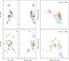 |
Fig. 1. 22 stellar groups recovered by EnLink. The vertical columns from left to right show the groups in 2D projection of celestial coordinates (right ascension and declination), parallax and declination, and proper motions. Due to the high number of groups, we show groups with at least 400 stars in the first row and the rest in the second row. Within each row, each color represents a distinct stellar group recovered by EnLink. The rest of the classified stars that do not fall into the size category in either row are shown as gray dots. EnLink recovers several stellar groups not shown in SNN results, including σ Ori, NGC 2024, and NGC 2068, as well as two spatially compact groups circled out in the sky in the second row. |
The small groups in the second row reveal that the automatic adaptive metric in EnLink assigns much more weight to RA, Dec and parallax than proper motions. The groups are much more coherent in the first two projections than in proper motion space. Because of this, EnLink recovers NGC 2024 (green) and NGC 2068 (purple) in Orion B and σ Ori (orange) as well as two other spatially compact groups which are missing from the SNN results. These groups were juedged by SNN to be unstable because of their large spreads in proper motion space. We are not overly concerned with SNN not recovering NGC 2024 and NGC 2068 because the goal of this work is to find new stellar groups. As for the two spatially compact groups, SNN recovered dozens of unstable groups similar to these so they are quite common occurrences with SNN. We decided not to discuss them in this work and focus on the most stable stellar groups.
Now we discuss the stellar groups from our two-stage SNN analysis as our final results. Figure 2 shows the SNN stellar groups in the same projections as Fig. 1. This time we place the groups into three rows to maximize their separation in 5D space instead of separating them by size. Again, we need to reuse colors to make these stellar groups distinguishable by sight. The opacity of points in Fig. 2 is coded by its frequentist membership probability and each group is assigned a numeric label according to its order of frequentist stability (Group 1 is the most stable) for easier identification. The SNN algorithm was able to recover almost all EnLink stellar groups, though the SNN counterparts contain more stars and appear more coherent in proper motion space. In Fig. 3, we further confirm that our SNN groups are coherent in 5D astrometric space by mapping the groups onto a 2D space with t-distributed Stochastic Neighbor Embedding (t-SNE; van der Maaten & Hinton 2008). The t-SNE algorithm is a common dimension reduction technique to help visualize structures in high-dimensional data and has been widely applied in astronomy (see Lin et al. 2019; Zhang et al. 2019; Kos et al. 2018). The most important feature of both the SNN and EnLink results is perhaps that most groups correspond to known structures in the Orion complex, which gives us confidence that the extraction of groups is physically meaningful.
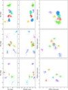 |
Fig. 2. 25 stellar groups recovered by SNN with our procedure to identify repeated groups in parameter space. Groups 13 and 18 are omitted as they appear to be duplicates of Group 3. The organization of the panels is exactly the same as in Fig. 1. The groups are presented in three rows to provide the maximum separation in the three projections. Distinct colors in each row represent distinct stellar groups. Again, it should be noted that the same colors are used to represent different groups in different rows. The stellar groups are assigned unique numeric label, which are also used in Table 1 to refer to each group. Compared to EnLink results in Fig. 1, the SNN stellar groups are slightly more spatially spread out but have much tighter distributions in proper motion space. |
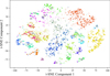 |
Fig. 3. SNN stellar groups in t-SNE 2D projection. Each stellar group is highlighted with a distinct color and a numeric label. The groups are coherent in this 2D space reduced from 5D astrometric space, affirming our results obtained from SNN. |
Stellar groups recovered by SNN.
An important implication of our results is the discovery that there are several distinct groups along the same line of sight, which is consistent to the argument in Alves & Bouy (2012). This is revealing of the overall architecture of the region but poses an obvious complication for studies of this region. An example is the area of the Orion Belt Population, or OBP (Kubiak et al. 2017), where at least five groups can be seen along the same general line of sight toward the Orion Belt stars with distinct proper motions. To give another example, Groups 6, 9, and 16 in the second row of Fig. 2 are adjacent in spatial coordinates but do not overlap at all in proper motion space. Comparing this to the results in Kounkel et al. (2018), we find that Orion D in is divided among at least Groups 1, 3, 7, 8, 9, 11, 20, and 23 in our results. These groups are distinct enough in proper motion space to be identified as individual groups, revealing a complex dynamical structure. Some of these groups were already identified in the past; Group 1 clearly clusters around 25 Ori (Briceño et al. 2007) and Group 20 matches Orion X (Bouy & Alves 2015). Follow-up work will investigate what these differences might mean in a global analysis of kinematics in the region.
We now discuss some of the more noteworthy groups. Group 1 coincides with the 25 Ori cluster (Briceño et al. 2007, 2018), although it appears much more elongated than previously assumed, reaching as far south as L1616. We note, however, that the distance to this group is about 350 pc, about 100 pc farther than the distance to the 25 Ori star, meaning that the star is probably not part of the cluster. To avoid confusion in the future when better data become available, we suggest naming the group Briceno 1, following the discovery paper Briceño et al. (2007).
Group 3 appears to be one of the richer groups as it contains Groups 13 and 18. However, we did not observe any significant offset among the three groups in the five input dimensions and thus chose to omit Groups 13 and 18. At a distance of about 360 pc, Group 3 lies toward the OBP (Kubiak et al. 2017) but is located towards the front, hence the OBP-near. Group 4 corresponds to the well-known λ Ori cluster of which Group 25 is a subgroup. However, a new group, Group 10, which we name λ Ori South, is clearly identified in the south of λ Ori and lies slightly beyond.
Group 5, or the NGC 1980 group, is one of the richer groups and it contains the disputed foreground population to the Orion Nebula Cluster (ONC). The group peaks around NGC 1980 and was discovered in Alves & Bouy (2012) and further extended in Bouy et al. (2014) (see Da Rio et al. 2016; Fang et al. 2017; Kounkel et al. 2017; Beccari et al. 2017; Jerabkova et al. 2019 for a different view). The group extends roughly from NGC 1981 down to south of NGC 1980, passing in front of the ONC and, in particular, the Trapezium cluster, which we do not manage to retrieve from Gaia DR2. The foreground of the ONC and the Trapezium is an important one, as this cluster is a benchmark for star formation studies, and an unrecognized foreground population compromises the basic properties derived for the region. Better data in Gaia EDR3 and, in particular, the large number of radial velocities available in Gaia DR3, should be able to clarify this situation and the actual position of Group 5 in relation to the ONC.
Group 7 corresponds to a layer in Blaauw’s sub-group Ia and was identified as ASCC 20 by Kos et al. (2018). The coordinates and parallax values of Group 7 also resemble the young population found in Zari et al. (2017). Group 8 lies below the OBP and extends to L1616, a small cometary cloud at the same distance which is currently star-forming (at least one source in the sample appears to belong to the small star-forming region). It is possible that this group formed from a cloud is now gone except for the leftover cometary cloud L1616, but more data would be needed to make this conclusion.
Group 11 seems to trace IC 2118, a faint and elongated reflection nebula of Rigel. It is likely that Rigel is part of this group as it overlaps with it in projection and is at about the same distance within the HIPPARCOS parallax error (the reason we name it the Rigel Group here), but this statement needs confirmation in future Gaia data releases.
Group 12, or the L1641S group, is associated with ongoing star formation toward the tail of the cloud, in particular the L1641S cluster. It is also associated with two smaller clusters toward the southern tail of the cloud and possibly Group 17 or L1647 (see Strom et al. 1993; Meingast et al. 2016; Großschedl et al. 2019).
Group 14, or the ome Ori group, is a dispersed group at about 417 pc, between Orion B and the λ Ori molecular ring. This group includes ome Ori, a Be star with a reflection nebula that is part of the group and is at about the same distance as the average distance of the group. Group 15, or L1562, to the west of the λ Ori group, lies at a distance of about 317 pc (i.e., about 100 pc in front of λ Ori). It might be associated with some of the leftover molecular material in the region, such as the small cometary cloud L1571 and the even smaller cloud L1562 at l, b = (187.2, −16.7), which lies close to the main clustering of sources in this group.
Group 16, or OBP-west, is a new, well-defined and centrally concentrated group at a distance of about 416 pc. It overlaps extensively with Group 1 (Briceno 1) but lies about 60 pc toward the back of the 25 Ori group. It is located west of the OBP and overlaps slightly with it so we name it OBP-west. Group 17 seems to coincide with the partially embedded young populations at the tail of Orion A, L1647, hence the name of the group, at a distance of about 450 pc (Großschedl et al. 2018a,b).
Group 19, OBP-far, is the farthest group along the line of sight to the Orion Belt. It is at a distance of about 426 pc. Group 21 includes the stellar yield of the L1634 cloud (e.g., Alcalá et al. 2008). It also contains a previously unknown population 1.5 degrees northwest of L1634, hence our naming it the L1634 group.
Groups 22 (Orion B East) and 24 (Orion A East) are dispersed groups located to the east of the Orion A and B clouds and are among the groups with lower stabilities. Group 24 is, surprisingly, the most distance of all the groups in this region beyond the Orion A cloud. If this cluster is young and formed in the larger Orion star-forming region, it would constitute an important clue that star formation in Orion did not happen in a linear and coherent manner, one producing a well-defined age gradient, but it more likely happened more chaotically.
4.2. Unclassified stars
Since SNN is based on DBSCAN which leaves out data points as noise, we briefly discuss the unclassified stars here. Figure 4 shows the unclassified stars in the same projection as Figs. 1 and 2. All unclassified stars are shown in gray by default, while those in four over-dense regions of the sky are highlighted in distinct colors. We wanted to understand why SNN did not assign labels to these stars and possibly identify any groups that SNN missed, besides the ones already found by EnLink.
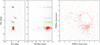 |
Fig. 4. Stars unclassified by SNN clustering algorithm. Stars in four over-dense regions of the sky are highlighted in distinct colors and examined across the same projections as Fig. 1. Spot 1 (red) targets the head of Orion A where Group 5 is recovered. A hole is visible in the proper motion space due to the classified stars in Group 5. Spots 2 and 3 target the OB1b and OB1a associations. Spot 4 targets λ Ori. No over-density in the proper motion space can be identified in these spots. We omit over-densities that correspond to σ Ori and Orion B here because they are already identified in Fig. 1. |
Spot 1 targets the head of Orion A where Group 5 is recovered. We limited membership probability to above 10% to eliminate sporadic members. A large number of stars were not picked up by SNN in this region. A hole is visible in the proper motion distribution due to the classified stars in Group 5. Therefore, SNN treated these stars as noise primarily because they are outliers in proper motions. Spots 2 and 3 target the OB1b and OB1a associations. Spot 4 targets the leftover stars from λ Ori. Similar to the stars in Spot 1, no over-density can be visually identified in proper motion space from these spots, even if we plot the spots individually to remove obscuring effects due to overlap. Overall, SNN did a satisfactory job removing over-densities from the astrometric 5D space.
5. Conclusion
We used the parameter-free EnLink as an exploratory tool and adopted the SNN algorithm to dissect the Orion star-forming complex. Our two-stage SNN procedure incorporates the within-source co-variance matrices and accomplishes three tasks commonly involved in clustering analysis, that is to say parameter tuning, computing group stability and assigning frequentist membership probability. We recovered 22 spatially and kinematically coherent unique stable groups in the Orion complex, as Groups 13, 18, and 25 appear to be only the highest or lowest density regions of their parent groups. Perhaps more remarkable, most of the unique groups identified in this work match previously well-known stellar populations, which gives us confidence in the approach. We find 12 new stellar groups, spread as far as about 150 pc in front of the star-forming Orion clouds, to about 50 pc beyond them. Here we unexpectedly find several groups, revealing the wealth of sub-structure in the OB association, within and beyond the classical Blaauw Orion OBI sub-groups Blaauw (1964), Brown et al. (1994), de Zeeuw et al. (1999).
The analysis in this work should be repeated including the sixth dimension, radial velocity, in the future. We expect radial velocity to be available for more stars in the Orion complex from Gaia DR3 or ongoing GALAH and APOGEE observations. Kos et al. (in prep.) will provide a chemical survey of the Orion star-forming complex with chemical abundances from newly observed GALAH data. The addition of radial velocity will allow us to produce stellar groups consistent in 6D phase space and study the kinematics of these groups more confidently. Gaia DR3 will provide more precise parallaxes and proper motions, which would further improve clustering results and allow us to identify finer structures in Orion. For now, a full characterization of the new groups is of essential as it offers the potential to unveil how star formation proceeds globally in large complexes such as Orion.
Acknowledgments
We thank the anonymous referee and Karolina Kubiak for their useful comments. B.C. is supported by the Research Training Program (RTP) offered by the Australian Department of Education. A.A. acknowledges the support of the Swedish Research Council, Vetenskapsrådet, and the Swedish National Space Agency (SNSA). This work has made use of data from the European Space Agency (ESA) mission Gaia (https://www.cosmos.esa.int/Gaia), processed by the Gaia Data Processing and Analysis Consortium (DPAC, https://www.cosmos.esa.int/web/Gaia/ dpac/consortium). Funding for the DPAC has been provided by national institutions, in particular the institutions participating in the Gaia Multilateral Agreement. This project was developed in part at the 2018 NYC Gaia Sprint, hosted by the Center for Computational Astrophysics of the Flatiron Institute in New York City and in part at the 2019 Santa Barbara Gaia Sprint, hosted by the Kavli Institute for Theoretical Physics at the University of California, Santa Barbara. This research was supported in part at KITP by the Heising-Simons Foundation and the National Science Foundation under Grant No. NSF PHY-1748958. We thank Josefa Großschedl for her detailed examination of the final draft.
References
- Alcalá, J. M., Covino, E., & Leccia, S. 2008, Handbook of Star Forming Regions, 64, 801 [Google Scholar]
- Alves, J., & Bouy, H. 2012, A&A, 547, A97 [NASA ADS] [CrossRef] [EDP Sciences] [Google Scholar]
- Astropy Collaboration (Robitaille, T. P., et al.) 2013, A&A, 558, A33 [NASA ADS] [CrossRef] [EDP Sciences] [Google Scholar]
- Astropy Collaboration (Price-Whelan, A. M., et al.) 2018, AJ, 156, 123 [Google Scholar]
- Bally, J. 2008, in Overview of the Orion Complex, ed. B. Reipurth, 4, 459 [Google Scholar]
- Beccari, G., Petr-Gotzens, M. G., Boffin, H. M. J., et al. 2017, A&AS, 604, A22 [Google Scholar]
- Blaauw, A. 1964, ARA&A, 2, 213 [Google Scholar]
- Bouy, H., & Alves, J. F. 2015, A&AS, 584, A26 [Google Scholar]
- Bouy, H., Alves, J., Bertin, E., Sarro, L. M., & Barrado, D. 2014, A&AS, 564, A29 [Google Scholar]
- Briceño, C., Hartmann, L., Hernández, J., et al. 2007, ApJ, 661, 1119 [NASA ADS] [CrossRef] [Google Scholar]
- Briceño, C., Calvet, N., Hernandez, J., et al. 2018, AJ, submitted [arXiv:1805.01008] [Google Scholar]
- Brown, A. G. A., de Geus, E. J., & de Zeeuw, P. T. 1994, A&A, 289, 101 [NASA ADS] [Google Scholar]
- Chen, B., D’Onghia, E., Pardy, S. A., et al. 2018, ApJ, 860, 70 [NASA ADS] [CrossRef] [Google Scholar]
- Da Rio, N., Tan, J. C., Covey, K. R., et al. 2016, ApJ, 818, 59 [NASA ADS] [CrossRef] [Google Scholar]
- de Zeeuw, P. T., Hoogerwerf, R., de Bruijne, J. H. J., Brown, A. G. A., & Blaauw, A. 1999, AJ, 117, 354 [NASA ADS] [CrossRef] [Google Scholar]
- Ertoz, L., Steinbach, M., & Kumar, V. 2003, in Proceedings of the Third SIAM International Conference on Data Mining (SDM 2003), eds. D. Barbara, & C. Kamath (Society for Industrial and Applied Mathematics), Proc. Appl. Math., 112 [Google Scholar]
- Ester, M., Kriegel, H. P., Sander, J., & Xu, X. 1996, Proceedings of the Second International Conference on Knowledge Discovery and Data Mining, KDD’96 (AAAI Press), 226 [Google Scholar]
- Fang, M., Kim, J. S., Pascucci, I., et al. 2017, ApJS, 153, 188 [NASA ADS] [CrossRef] [Google Scholar]
- Gaia Collaboration (Prusti, T., et al.) 2016, A&A, 595, A1 [NASA ADS] [CrossRef] [EDP Sciences] [Google Scholar]
- Gaia Collaboration (Brown, A. G. A., et al.) 2018, A&A, 616, A1 [NASA ADS] [CrossRef] [EDP Sciences] [Google Scholar]
- Großschedl, J. E., Alves, J., Meingast, S., et al. 2018a, A&AS, 619, A106 [NASA ADS] [CrossRef] [EDP Sciences] [Google Scholar]
- Großschedl, J. E., Alves, J., Meingast, S., & Hasenberger, B. 2018b, IAU Conf. Proc. IAUS345, submitted [arXiv:1812.08024] [Google Scholar]
- Großschedl, J. E., Alves, J., Teixeira, P. S., et al. 2019, A&A, 622, A149 [NASA ADS] [CrossRef] [EDP Sciences] [Google Scholar]
- Jerabkova, T., Beccari, G., Boffin, H. M. J., et al. 2019, A&A, 627, A57 [NASA ADS] [CrossRef] [EDP Sciences] [Google Scholar]
- Kharchenko, N. V., Piskunov, A. E., Schilbach, E., Röser, S., & Scholz, R. D. 2013, A&A, 558, A53 [NASA ADS] [CrossRef] [EDP Sciences] [Google Scholar]
- Kos, J., Bland-Hawthorn, J., Freeman, K., et al. 2018, MNRAS, 473, 4612 [NASA ADS] [CrossRef] [Google Scholar]
- Kounkel, M., Hartmann, L., Calvet, N., & Megeath, T. 2017, AJ, 154, 29 [NASA ADS] [CrossRef] [Google Scholar]
- Kounkel, M., Covey, K., Suárez, G., et al. 2018, AJ, 156, 84 [NASA ADS] [CrossRef] [Google Scholar]
- Kubiak, K., Alves, J., Bouy, H., et al. 2017, A&AS, 598, A124 [NASA ADS] [CrossRef] [EDP Sciences] [Google Scholar]
- Lin, J., Asplund, M., Ting, Y. S., et al. 2019, MNRAS, 491, 2043 [CrossRef] [Google Scholar]
- Majewski, S. R., Schiavon, R. P., Frinchaboy, P. M., et al. 2017, AJ, 154, 94 [NASA ADS] [CrossRef] [Google Scholar]
- Meingast, S., Alves, J., Mardones, D., et al. 2016, A&AS, 587, A153 [NASA ADS] [CrossRef] [EDP Sciences] [Google Scholar]
- Murdin, P., & Penston, M. V. 1977, MNRAS, 181, 657 [NASA ADS] [CrossRef] [Google Scholar]
- Sharma, S., & Johnston, K. V. 2009, ApJ, 703, 1061 [NASA ADS] [CrossRef] [Google Scholar]
- Strom, K. M., Strom, S. E., & Merrill, K. M. 1993, ApJ, 412, 233 [NASA ADS] [CrossRef] [Google Scholar]
- van der Maaten, L., & Hinton, G. 2008, J. Mach. Learn. Res., 9, 2579 [Google Scholar]
- Zari, E., Brown, A. G. A., de Bruijne, J., Manara, C. F., & de Zeeuw, P. T. 2017, A&A, 608, A148 [NASA ADS] [CrossRef] [EDP Sciences] [Google Scholar]
- Zari, E., Brown, A. G. A., & de Zeeuw, P. T. 2019, A&A, 628, A123 [Google Scholar]
- Zhang, S., Zhang, S., Li, S., Du, L., & Habetler, T. G. 2019, ArXiv e-prints [arXiv:1911.01024] [Google Scholar]
All Tables
All Figures
|
Fig. 1. 22 stellar groups recovered by EnLink. The vertical columns from left to right show the groups in 2D projection of celestial coordinates (right ascension and declination), parallax and declination, and proper motions. Due to the high number of groups, we show groups with at least 400 stars in the first row and the rest in the second row. Within each row, each color represents a distinct stellar group recovered by EnLink. The rest of the classified stars that do not fall into the size category in either row are shown as gray dots. EnLink recovers several stellar groups not shown in SNN results, including σ Ori, NGC 2024, and NGC 2068, as well as two spatially compact groups circled out in the sky in the second row. |
| In the text | |
|
Fig. 2. 25 stellar groups recovered by SNN with our procedure to identify repeated groups in parameter space. Groups 13 and 18 are omitted as they appear to be duplicates of Group 3. The organization of the panels is exactly the same as in Fig. 1. The groups are presented in three rows to provide the maximum separation in the three projections. Distinct colors in each row represent distinct stellar groups. Again, it should be noted that the same colors are used to represent different groups in different rows. The stellar groups are assigned unique numeric label, which are also used in Table 1 to refer to each group. Compared to EnLink results in Fig. 1, the SNN stellar groups are slightly more spatially spread out but have much tighter distributions in proper motion space. |
| In the text | |
|
Fig. 3. SNN stellar groups in t-SNE 2D projection. Each stellar group is highlighted with a distinct color and a numeric label. The groups are coherent in this 2D space reduced from 5D astrometric space, affirming our results obtained from SNN. |
| In the text | |
|
Fig. 4. Stars unclassified by SNN clustering algorithm. Stars in four over-dense regions of the sky are highlighted in distinct colors and examined across the same projections as Fig. 1. Spot 1 (red) targets the head of Orion A where Group 5 is recovered. A hole is visible in the proper motion space due to the classified stars in Group 5. Spots 2 and 3 target the OB1b and OB1a associations. Spot 4 targets λ Ori. No over-density in the proper motion space can be identified in these spots. We omit over-densities that correspond to σ Ori and Orion B here because they are already identified in Fig. 1. |
| In the text | |
Current usage metrics show cumulative count of Article Views (full-text article views including HTML views, PDF and ePub downloads, according to the available data) and Abstracts Views on Vision4Press platform.
Data correspond to usage on the plateform after 2015. The current usage metrics is available 48-96 hours after online publication and is updated daily on week days.
Initial download of the metrics may take a while.