| Issue |
A&A
Volume 642, October 2020
|
|
|---|---|---|
| Article Number | A160 | |
| Number of page(s) | 9 | |
| Section | Extragalactic astronomy | |
| DOI | https://doi.org/10.1051/0004-6361/202039129 | |
| Published online | 15 October 2020 | |
Constraining the transient high-energy activity of FRB 180916.J0158+65 with Insight–HXMT follow-up observations
1
Department of Physics and Earth Science, University of Ferrara, Via Saragat 1, 44122 Ferrara, Italy
2
INFN – Sezione di Ferrara, Via Saragat 1, 44122 Ferrara, Italy
e-mail: This email address is being protected from spambots. You need JavaScript enabled to view it.
3
INAF – Osservatorio di Astrofisica e Scienza dello Spazio di Bologna, Via Piero Gobetti 101, 40129 Bologna, Italy
4
Key Laboratory of Particle Astrophysics, Institute of High Energy Physics, Chinese Academy of Sciences, 19B Yuquan Road, Beijing 100049, PR China
5
University of Chinese Academy of Sciences, Chinese Academy of Sciences, Beijing 100049, PR China
6
Department of Astronomy, Beijing Normal University, Beijing 100088, PR China
7
Department of Astronomy, Tsinghua University, Beijing 100084, PR China
8
Computing Division, Institute of High Energy Physics, Chinese Academy of Sciences, 19B Yuquan Road, Beijing 100049, PR China
9
Key Laboratory of Space Astronomy and Technology, National Astronomical Observatories, Chinese Academy of Sciences, Beijing 100012, PR China
10
College of physics Sciences and Technology, Hebei University, No. 180 Wusi Dong Road, Lian Chi District, Baoding City, Hebei Province 071002, PR China
11
School of Physics and Optoelectronics, Xiangtan University, Yuhu District, Xiangtan, Hunan 411105, PR China
Received:
9
August
2020
Accepted:
26
August
2020
Abstract
Context. A link has finally been established between magnetars and fast radio burst (FRB) sources. Within this context, a major issue that remains unresolved pertains to whether sources of extragalactic FRBs exhibit X/γ-ray outbursts and whether this is correlated with radio activity. If so, the subsequent goal is to identify these sources.
Aims. We aim to constrain possible X/γ-ray burst activity from one of the nearest extragalactic FRB sources currently known. This is to be done over a broad energy range by looking for bursts over a range of timescales and energies that are compatible with those of powerful flares from extragalactic magnetars.
Methods. We followed up on the observation of the as-yet nearest extragalactic FRB source, located at a mere 149 Mpc distance, namely, the periodic repeater FRB 180916.J0158+65. This took place during the active phase between 4 and 7 February 2020, using the Insight–Hard X-ray Modulation Telescope (Insight–HXMT). By taking advantage of the combination of broad-band wavelengths, a large effective area, and several independent detectors at our disposal, we searched for bursts over a set of timescales from 1 ms to 1.024 s with a sensitive algorithm that had been previously characterised and optimised. Moreover, through simulations, we studied the sensitivity of our technique in the released energy-duration phase space for a set of synthetic flares and assuming a range of different energy spectra.
Results. We constrain the possible occurrence of flares in the 1−100 keV energy band to E < 1046 erg for durations Δ t < 0.1 s over several tens of ks exposure.
Conclusions. We can rule out the occurrence of giant flares similar to the ones that were observed in the few cases of Galactic magnetars. The absence of reported radio activity during our observations prevents us from making any determinations regarding the possibility of simultaneous high-energy emission.
Key words: radiation mechanisms: non-thermal / stars: magnetars
© ESO 2020
1. Introduction
Fast radio bursts (FRBs) are a new class of ms-long radio flashes of unknown extragalactic origin. The determination of their host galaxy identification and redshift have become feasible in recent years by way of several cases (Tendulkar et al. 2017; Bannister et al. 2019; Prochaska et al. 2019; Ravi et al. 2019; Marcote et al. 2020; Macquart et al. 2020). The combination of the three properties of short duration, specific luminosity (≲1034 erg s−1 Hz−1), and brightness temperature (Tb ≳ 1035 K) suggests that the progenitor is a compact source emitting through a coherent process (see Cordes & Chatterjee 2019; Petroff et al. 2019 for recent reviews).
Following the discovery of repeating FRB sources, in particular (Spitler et al. 2016; CHIME/FRB Collaboration 2019a,b; Kumar et al. 2019; Fonseca et al. 2020), magnetars caught further attention as one of the most promising candidates (Popov & Postnov 2010; Lyubarsky 2014; Beloborodov 2017; Metzger et al. 2019). On the theoretical side, connections with sources of gamma-ray bursts (GRBs) have not been ruled out (see Platts et al. 2019 for a review of theoretical models), as young ms-magnetars could be the endpoint of GRB progenitors (Usov 1992; Thompson 1994; Bucciantini et al. 2007; Metzger et al. 2011) and cataclysmic models cannot be ruled out as long as one-off FRBs are consistently observed. Nonetheless, observations carried out so far appear to exclude a systematic link between FRBs and standard cosmological GRBs (Tendulkar et al. 2016; Guidorzi et al. 2019, 2020; Martone et al. 2019; Cunningham et al. 2019; Anumarlapudi et al. 2020). The possibility, as suggested by Ravi & Lasky (2014), that a FRB could result from the final collapse of a newborn supramassive neutron star some 10 to 104 s after a binary neutron star merger, which would be signalled by a short GRB, found no confirmation through the search for FRB counterparts in the case of four promptly localised short GRBs (Bouwhuis et al. 2020).
The extreme magnetic field (B ∼ 1014 − 1015 G) of magnetars is thought to power their high-energy emission, which is characterised by periods of quiescence, interspersed with active intervals described by sporadic short X-ray bursts (typical duration of ∼0.1 s) with luminosities in the range 1036 − 1043 erg s−1, and rarely by giant flares (GFs). These consist of an initial short spike with a peak luminosity in the range of 1044 − 1047 erg s−1, followed by a several-hundred-second-long fainter tail modulated by the star’s spin period. Only three GFs from magnetars, two in the Galaxy, and one in the Large Magellanic Cloud, have been observed so far, although a few extragalactic candidates have also been reported (Frederiks et al. 2007a, 2020; Mazets et al. 2008; Svinkin et al. 2020; Yang et al. 2020). See Turolla et al. (2015), Mereghetti et al. (2015), Kaspi & Beloborodov (2017) for reviews on magnetars.
For most FRBs, the possibility of a simultaneous magnetar GF could not be discarded, mainly due to the limited sensitivity of past or currently flying γ-ray detectors, combined with FRB distances (e.g. Martone et al. 2019; Guidorzi et al. 2019, 2020). However, neglecting possible different beaming factors between radio and high-energy emission, a one-to-one correspondence between FRBs and magnetar GFs has to be excluded because of the meaningful lack of a radio detection associated with the most luminous Galactic GF observed thus far (Tendulkar et al. 2016).
A turning point recently came with the discovery of Galactic FRB 200428, simultaneously with a hard X-ray burst from the recently reactivated magnetar SGR 1935+2154 (Li et al. 2020; Mereghetti et al. 2020; Ridnaia et al. 2020); as seen with the Canadian Hydrogen Intensity Mapping Experiment (CHIME; CHIME/FRB Collaboration 2019a), the FRB consists of two peaks that are 30 ms apart, with an energy of 3 × 1034 erg and peak luminosity of 7 × 1036 erg s−1 in the 400−800 MHz band (CHIME/FRB Collaboration 2020a). It was also detected with the Survey for Transient Astronomical Radio Emission 2 (STARE2; Bochenek et al. 2020a) in the 1281−1468 MHz band with a burst energy of 2 × 1035 erg and a luminosity of 4 × 1038 erg s−1 (Bochenek et al. 2020b). This FRB is ∼40 times less energetic than the least energetic extragalactic sample measured thus far. The X/γ-ray counterpart also consists of two main peaks temporally coincident with their radio analogues, that is, once the delay expected from the dispersion measure is accounted for. Interestingly, while the released energy is typical of magnetar bursts, this event exhibits an unusually structured, slowly rising time profile when compared with that of a typical short burst. In addition, its spectrum, which is unusually hard as well, is fitted with a cutoff power-law with photon index between 0.4 and 1.6 and cutoff energy in the range 65 − 85 keV, corresponding to a released energy of 1 × 1040 erg and peak luminosity of 1 × 1041 erg s−1 (Li et al. 2020; Ridnaia et al. 2020). This FRB followed an intense hard X-ray burst activity which had culminated with a burst forest on April 27, 2020 (Palmer 2020; Younes et al. 2020). On the one hand, this event finally provided direct evidence that at least some FRBs originate in magnetars, along with hard X-ray bursts; on the other hand, the lack of radio counterparts to many other hard X-ray bursts from the same source, with upper limits that are 108 times fainter than FRB 200428, demonstrates the rarity of this kind of joint emission (Lin et al. 2020).
The discovery of FRB 180916.J0158+65, the as-yet nearest extragalactic FRB source with measured redshift, at a luminosity distance of 149.0 ± 0.9 Mpc (Marcote et al. 2020), which was also found to be a repeater, made it a desirable target for multi-wavelength surveys. The subsequent discovery of a periodic modulation in its radio burst activity with P = 16.35 ± 0.15 days, with a FRB rate of up to ∼1 h−1 for a ±2.7 day window around peak (CHIME/FRB Collaboration 2020b), led to the planning of multi-wavelength campaigns around the expected peaks. In a 33 ks Chandra X-ray Observatory observation, which covered one FRB detected with CHIME, the study by Scholz et al. (2020) detected no X-ray source, with upper limits on the released energy of 1.6 × 1045 erg and 4 × 1045 erg at the FRB time and at any time, respectively, in the 0.5 − 10 keV energy band. They also derived an upper limit of 6 × 1046 erg in the 10 − 100 keV band for 12 bursts from FRB 180916.J0158+65 that were visible with Fermi/Gamma-ray Burst Monitor (GBM; Meegan et al. 2009). The XMM-Newton detected no source down to E < 1045 erg in the 0.3 − 10 keV energy band at the times of three radio bursts, which were discovered at 328 MHz with the Sardinia Radio Telescope (Pilia et al. 2020). Comparable upper limits of 3 × 1046 erg on the energy released in the optical band, simultaneous with FRBs, from FRB 180916.J0158+65 were also derived in a statistical framework using survey data from the Zwicky Transient Facility (Andreoni et al. 2020).
The Hard X-ray Modulation Telescope (HXMT), named “Insight” after its launch on 15 June 2017, is the first Chinese X-ray astronomy satellite (Li 2007; Zhang 2020). On board, it carries three main instruments: the Low Energy X-ray telescope (LE; 1−15 keV; Chen et al. 2020), the Medium Energy X-ray telescope (ME; 5−30 keV; Cao et al. 2020), and the High Energy X-ray telescope (HE; Liu et al. 2020). The HE consists of 18 NaI/CsI detectors covering the 20−250 keV energy band for pointing observations. Moreover, it also works as an all-sky monitor in the 0.2 − 3 MeV energy range. The unique combination of a very large geometric area (∼5100 cm2) with continuous event tagging, with a timing accuracy of < 10 μs, had already been exploited in the search for possible γ-ray counterparts to a sample of 39 FRBs down to ms or sub-ms scales in the keV–MeV energy range. As a result, the association with cosmological GRBs was excluded on a systematic basis (Guidorzi et al. 2020, hereafter G20).
In this work, we report the results of follow-up observations of FRB 180916.J0158+65 that were carried out with Insight–HXMT around one of the expected peaks of radio activity between 4 and 7 February 2020, for which no observations had been reported to date. Section 2 describes the data set and reduction. Our analysis is presented in Sect. 3. Results are in given in Sect. 4 and discussed in Sect. 5. We present our conclusions in Sect. 6.
2. Data set
Insight–HXMT observed the FRB 180916.J0158+65 from 2020-02-04 12:40:19 to 2020-02-07 07:39:44 UT as a target of opportunity observation, which had been requested in correspondence of a predicted maximum from radio observations. The detailed log of the Insight–HXMT observation is listed in Table 1. The different net exposures of the instruments are due to the filtering criteria adopted for the generation of the good time intervals.
Log of the Insight–HXMT observation of FRB 180916.J0158+65.
For our analysis, we used the software package HXMTDAS version 2.02.11. The screening of the raw events was performed by means of the legtigen, megtigen, and hegtigen tasks2. Standard filtering criteria were adopted, namely: the Earth elevation angle ELV > 10 deg; the cutoff rigidity COR > 8 GeV; the pointing offset angle ANG_DIST < 0.04 deg. We also excluded data taken close to the South Atlantic Anomaly (SAA) by selecting T_SAA and TN_SAA both greater than 300 s. For the LE instrument, we selected only data for which the Bright Earth Angle was greater than 30 deg.
From the cleaned event files, we then extracted the light curves with 1 ms time resolution. For the HE instrument, we also extracted the light curves for each HE unit to improve the efficiency of the multi-detector-search algorithm to the LE+ME+HE light curves.
Because of the uncertainties in the background evaluation (as made evident by the net count rates listed in Table 1) performed by the tasks lebkgmap (Liao et al. 2020), mebkgmap (Guo et al. 2020), and hebkgmap (Liao et al. 2020), the background was evaluated by applying a procedure that interpolates the background starting from a 10 s binned light curve, applying polynomials with increasing order to individual orbits up to the point where both χ2 and runs tests (2-tails) had a P-value > 0.01, so as to avoid both under- and over-fitting. The time bins for which this procedure was not able produce the required P-values were discarded. The resulting net exposure is also reported in Table 1. Consequently, this procedure can only detect relatively short bursts, whereas a possible relatively faint, constant source, or varying over timescales > 10 s cannot be detected.
Table 1 also reports the net exposure for each combination of instruments whose data are available simultaneously: only the LE and HE combination without ME does not appear to have a significant exposure. We included the time intervals for which only HE data are available because the multiplicity of its independent detectors still enables an effective search for transients. With regard to the HE, in the following, we ignored the blocked collimator detector, which was devised to measure the local background of HE (Liu et al. 2020), therefore using the data from the remaining 17 detectors. Hereafter, only the filtered time bins for each instrument are considered in the analysis.
There is no FRB reported during our observations: specifically, on 4 February 2020, CHIME reported four bursts, last one at 01:17:21.37 UT, thus, more than 11 h before the beginning of Insight–HXMT observations. The next FRB reported by CHIME from this source was 15 days later3. Assuming a period of 16.35 days, the expected peak of radio activity considered by us was at 2020-02-05 04:55 UT: the Insight–HXMT observing window spans the time interval from −0.7 to 2.1 days around it, so completely within the ±2.7 day interval characterised by the expected peak burst rate of 1.0 ± 0.5 h−1 (CHIME/FRB Collaboration 2020b). The total net exposure used in the present work is 0.65 days, which corresponds to 23% of the overall observing window.
3. Data analysis
A transient increase of the count rate of the detectors may be caused by two different kinds of phenomena: (i) an electromagnetic wave associated with a transient event, whose photons interact with a number of detectors; (ii) high-energy charged particles interacting with individual detectors. The main distinctive property of the electromagnetic wave is a common spectral and temporal evolution as recorded by the different detectors, whereas the particle-induced event deposits its energy in one or a few detectors and in an uncorrelated way, resulting in spikes in the count rates that are significantly in excess of what is expected from the counting statistics. In particular, when dim astrophysical transients and short integration times are considered, the very few expected counts can be easily confused with particle spikes. Consequently, searching for simultaneous excesses over a number of detectors is the most effective way for distinguishing them.
To this aim, G20 developed the so-called multi-detector search (MDS) method meant to exploit the segmented nature of the Insight–HXMT/HE instrument to search for transient candidates that are possibly associated with FRBs. While it was only CsI events that were considered in that case (as they were transparent to the collimators), the data analysed here are taken from a pointed observation and mainly differ in two aspects: (1) concerning the HE, we consider NaI rather than CsI events; (2) data from the other two instruments operating in the corresponding softer energy bands are included. In light of this, we had to tweak and adapt the original MDS algorithms as described below. In order to find the optimal compromise between sensitivity and false positive rate, we preliminarily characterised the background statistical properties for each detector.
3.1. Background statistical properties
Prior to investigating the nature of possible candidates, we assumed that their signal does not affect the overall count distribution since the great majority of the recorded counts is assumed to be the background. For each of the 19 detectors (LE, ME, and 17 HE-NaI units), we accumulated the overall 1 ms count distribution. In order to test whether this is compatible with a statistical realisation of a variable Poisson process, whose expected value for each time bin is given by the locally estimated background, we simulated 100 realisations for each bin. For each detector, we thus ended up with a distribution of expected counts having 100 times as many bins as the corresponding real one.
We then compared each of the 19 real count distributions with their corresponding synthetic ones. As a result, the total recorded counts are slightly, but significantly, in excess of pure Poisson noise by the following amounts: 1.2%, 0.6%, and 0.5% for the LE, ME, and average HE, respectively. These are caused by the occasional presence of spikes that are visible in individual detectors or another incompatibility with the signal that is expected from a plane wave. We also found that a possible way to reject most of them is by increasing the lower threshold on the photon energy, at least for the HE units.
Although this excess component accounts for ≲1% of the total background variance, it can affect the estimate of the statistical significance of peaks in the light curves, especially at short (∼few ms) integration times. It must be therefore taken into account when calculating the expected false positive rate. More details are reported in Appendix A.
3.2. Multi-detector search
The diversity of the three instruments and energy bands, coupled with the different combinations of available data shown in Table 1, forced us to conceive of a set of three complementary trigger criteria that address several alternative cases in which a candidate can be found, in principle. For each case, the philosophy is the same as that of the MDS, conceived in G20: for a given criterion, the threshold that must be exceeded by the counts for a generic bin depends on (a) the local interpolated background; (b) the integration time; (c) the minimum number of detectors to be triggered simultaneously, so as to end up with a desired combined probability. In addition, in the present work, the threshold must also depend on the kind of detector as well as on the data available at any given time bin. Following these guidelines, for each case, we have come up with a set of thresholds, expressed in units of Gaussian σ’s, following the same convention as in G20. Overall, a candidate must fulfil at least one trigger criterion. A detailed description is reported in Appendix B.
Due to the presence of a small, but significant extra-Poissonian variance in the background counts (Sect. 3.1), we had to ensure that the false positive rate was not underestimated or, equivalently, that the confidence level of any possible candidate is not overestimated. Therefore, we further calibrated the thresholds by running the MDS on 100 synthetic samples that were obtained by shuffling all the 1 ms bins along with their associated counts and expected background counts for any detector, independently. This procedure preserves the properties of the count distribution for each detector, while, at the same time, it offers a way to calculate the probability for any possible combination of simultaneous excesses in different detectors. In this way, we ended up with a robust procedure for estimating the related multivariate probability distribution, having relaxed any assumption on the nature of the statistical noise of any individual detector. More details can be found in Appendix B. Not only can the MDS be used for other FRB sources that will be targeted by Insight–HXMT, but it may also help identify bursts from other sources not necessarily related to FRBs, such as weak, short GRBs that are possibly associated with gravitational-wave sources.
4. Results
Table 2 reports the results of the number of candidates as a function of the integration time along with the corresponding number of expected false positives, which already accounts for the multi-trials related to the total number of time bins that were screened. We found only one candidate from the screening of 10 ms time bins, centred at 2020-02-06 23:54:55.793 UT: with reference to the three MDS criteria (Appendix B), this event triggered criterion 2, that is, both LE and ME exceeded their thresholds, while only one of the HE units did. Should this be real, it would be a relatively spectrally soft event. The number of expected false positives for 10 ms integration time is 0.10, so that the chance probability of having at least one fake candidate is 9.5%. More correctly, when the same probability is calculated taking into account the trials related to all the explored integration times together, the total number of expected false positives rises to 1.06, indicating that it is fully consistent with the only candidate. In order to better evaluate its nature, we also inspected its counts in both LE and ME, and found that they were just above the respective thresholds. We found no simultaneous events reported by Fermi/GBM, INTEGRAL SPI-ACS, Swift/BAT, and Konus/WIND. The search for coincident subthreshold triggers in the case of Fermi/GBM4 and of Swift/BAT5 did not give any results either. Overall, we conclude that based on Insight–HXMT data alone, we cannot reject the possibility that the candidate is not astrophysical.
Number of candidates and expected false positives as a function of the integration time.
4.1. Upper limits and technique sensitivity
Given the lack of any confident detection of transient candidates with durations in the range 10−3 − 1 s, we derived corresponding upper limits on fluence as a function of duration by assuming three different energy spectra: a non-thermal power-law with photon index, Γ = 2, which is often found to adequately describe the photon spectrum of high-energy transient events, and an optically thin thermal bremsstrahlung (hereafter, OTTB), dN/dE ∝ E−Γ exp( − E/E0), with index, Γ = 1, and two different values for the cutoff energy, E0: 200 and 50 keV. Concerning the cutoff power-law, we opted for an OTTB, because it was adopted to fit the initial spikes of the few Galactic magnetar giant flares (Mazets et al. 1999; Feroci et al. 1999; Hurley et al. 1999, 2005; Palmer et al. 2005; Frederiks et al. 2007b), some extragalactic magnetar giant flare candidates (Frederiks et al. 2007a, 2020; Mazets et al. 2008), as well as the hard X-ray burst from SGR 1935+2154 associated with FRB 200428, when Γ is left free to vary from 1 (Li et al. 2020; Ridnaia et al. 2020; Mereghetti et al. 2020).
We then characterised the sensitivity of the MDS as follows: we defined a grid of points in the F − Δ t plane, where F is the 1−100 keV fluence and Δ t is the duration of a hypothetical transient. For each spectral model and for each point of this grid, we simulated 200 synthetic transients, which were added to the real counts at a given set of times that were uniformly distributed along the entire observing window, and then counted how many of them were identified by the MDS. The results for the OTTB with E0 = 50 keV and for the power-law are shown in the contour plots of Fig. 1. The results for the OTTB with E0 = 200 keV are omitted for the sake of clarity because they are intermediate between the other two. We also calculated the corresponding isotropic-equivalent released energy in the same energy band, Eiso (right-hand vertical axes in Fig. 1), at the distance of FRB 180916.J0158+65 and, in addition, we show the lines corresponding to a constant luminosity for three different values: 1046, 1047, and 1048 erg s−1. Looking at the regions with 90% probability for a transient to be detected, for events as short as a few ms, the minimum detectable energies are ∼1045.6 = 4 × 1045 erg. In terms of luminosity, the corresponding minimum values are a few ×1048 erg s−1. Considering longer transients, up to ∼0.1 s, the minimum detectable energy and luminosity values become respectively ∼1046 erg and 1047 erg s−1 in the worst case.
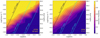 |
Fig. 1. Detection probability for a flare as a function of duration, Δ t, fluence, F (left-hand y axis), and isotropic–equivalent released energy, Eiso (right-hand y axis) in the 1−100 keV energy band for two different energy spectra: an OTTB with kT = 50 keV (left) and a power-law with photon index, Γ = 2 (right). The different solid lines correspond to constant luminosity values. |
4.2. Detection of radio bursts during Insight–HXMT observations
Although no radio burst has been reported to date during the Insight–HXMT observing window, it is worth estimating the probability that FRB 180916.J0158+65 gave no FRBs. Ignoring the complex dependence on frequency (CHIME/FRB Collaboration 2020b; Pilia et al. 2020; Chawla et al. 2020), here we focus on the homogeneous sample detected with CHIME.
Considering the ±0.9 d interval centred on the peak of radio activity, which has a burst rate of  h−1 (CHIME/FRB Collaboration 2020b), the net exposure of Insight–HXMT is ∼8.5 h. The probability of no FRBs over the duration of the Insight–HXMT observation is 2 × 10⁻⁴ at most. This would suggest that Insight–HXMT observations covered one FRB at least and, likely, a few of them (the probability of ≤2 FRBs is < 1%). This holds true as long as a constant burst rate is assumed for the same window around all peaks. While it was already shown that the burst rate changes significantly for windows with different durations around the peak times (CHIME/FRB Collaboration 2020b), nothing has been said on whether the constant rate assumption for a given window over different peak times is compatible with observations.
Therefore, we tested this possibility by taking the CHIME exposures from 28 August 2018 to 30 September 2019, for which data are available6. There are 19 radio bursts detected with CHIME within the ±0.9 d window around as many peaks7. To each peak, i, we assigned the probability, pi = Ei/E, for a burst to occur within its ±0.9 d window, where Ei is the exposure of that window and E = ∑iEi is the total exposure. From the multinomial distribution we then calculated the information I of the real sample {Ni}, where Ni is the number of FRBs observed in window i as follows:
 (1)
(1)
where N = ∑iNi = 19. We then generated 105 samples with N FRBs distributed over the same exposures and compared the distribution of the simulated information content with the real value. As a result, it is only for 1.7% of simulated samples that the data was higher than the real one. In other words, under the assumption of a constant rate around all peaks, the probability of having a distribution equal to or less probable than the observed one is 1.7%, equivalent to 2.4σ (Gaussian). In conclusion, although this assumption cannot be rejected with the present data, it suggests that different periods could be characterised by different radio activity at the peak. Very recently, the upgraded Giant Metrewave Radio Telescope (uGMRT; Gupta et al. 2017) detected 15 bursts from FRB 180916.J0158+65 in three successive cycles and found extreme variability during the active phase around peak (Marthi et al. 2020). Should this finding be strengthened by future data, we cannot reject the possibility that FRB 180916.J0158+65 did not emit a single FRB during these Insight–HXMT observations.
5. Discussion
The discovery of FRB 200428, a sub-energetic FRB from the recently reactivated Galactic source, SGR 1935+2154, provided the first compelling evidence that magnetars can, in fact, occasionally act as FRB sources. The question as to whether they are also responsible for the more energetic extragalactic siblings of FRB 200428 is still an open one. In particular, some extragalactic FRBs could be due to the most energetic subset of the magnetar population, which, in principle, could be way more energetic than the Galactic sources known thus far (Margalit et al. 2020). A possibility is offered by young (age ≲ 109 s), hyperactive magnetars with internal fields, B ∼ B16 × 1016 G, and magnetic energy reservoir of  erg (Beloborodov 2017), especially, for example, those that can be formed in compact mergers and whose magnetic activity would be enhanced by the large differential rotation at birth (Beloborodov 2020). As a result, the search for magnetar burst activity from known extragalactic FRB sources has gained prominence.
The initial spikes of giant flares from Galactic magnetars observed thus far have L ≲ 1047 erg s−1, E ≲ 1046 erg, and durations of Δ t ≲ 0.1 s (Mazets et al. 1979, 1999; Feroci et al. 1999; Hurley et al. 1999, 2005; Palmer et al. 2005). When giant flare candidates of extragalactic origin are considered, the observed released energies and luminosities can be larger by more than one order of magnitude (e.g. Mazets et al. 2008). In this context, our upper limits exclude the occurrence of giant flares that are either similar to or even more energetic than the brightest ones observed from known Galactic magnetars, at least during 23% of the three-day window centred on one of the peaks of the expected radio burst activity of FRB 180916.J0158+65. This holds true regardless of the possible simultaneous occurrence of radio bursts.
Hard X-ray bursts as energetic as the one associated with Galactic FRB 200428 are way below our sensitivity limits and, in any case, could not be detected. Even assuming the same γ-to-radio fluence ratio, which lies in the range of 5 × 10⁴ − 3 × 10⁵, and rescaling the energy range of FRB 180916.J0158+65 radio bursts (1037 − 4 × 1038 erg), each potentially associated high-energy burst should have E ∼ 3 × 1042 − 1044 erg, which is below our limits.
The fine temporal coincidence between radio and hard X-rays in the case of SGR 1935+2154 points towards a causal link between the two. The fact that the hard X-ray burst also exhibits some unusual features, such as its temporal profile and the spectral hardness, makes it likely to be connected to the rarity of the joint manifestation. High-energy bursts are thought to originate in the magnetar magnetosphere as a result of some twisting and buildup of free magnetic energy, which is suddenly released through reconnection and consequent pair plasma acceleration. These processes could either be induced by crustal fractures or be magnetospheric in origin (Lyutikov 2003), where the former seems to be favoured in the case of GFs (Feroci et al. 2001; Hurley et al. 2005). In this context, FRBs could be coherent curvature radiation from pairs (Katz 2014; Kumar et al. 2017; Yang & Zhang 2018) or due to an as-yet-unidentified process (Lyutikov & Popov 2020). In any case, this would involve a scenario that would account for the simultaneity of radio and hard X-rays in the magnetosphere (Li et al. 2020). Alternatively, FRBs could be synchrotron maser radiation caused by relativistic magnetised shocks driven by plasmoids at outer radii (1014 − 1016 cm), which were launched by flares (Lyubarsky 2014; Beloborodov 2017, 2020; Metzger et al. 2019). In this scenario, FRBs would be much more collimated than the high-energy emission due to relativistic beaming of the plasmoids: this would explain both the negligible time delay between radio and hard X-rays, as well as the rarity of the FRB emission associated with magnetar bursts. Besides, the energy ratio between flare and the associated FRB, ∼105, is compatible with the expected radiative efficiency (Plotnikov & Sironi 2019; Beloborodov 2020).
While FRB 200428 could belong to the low-energy tail of the extragalactic FRB energy distribution, which cannot be explored at cosmological distances with the current instrumentation (Bochenek et al. 2020b), the question whether the same mechanism that is at play for SGR 1935+2154 can be scaled up by four to six decades for the case of GFs remains open and, therefore, justifies the search for them among FRB sources.
The origin of the periodicity found in the radio activity of FRB 180916.J0158+65, which might also relate to the case of FRB 121102 (Rajwade et al. 2020), along with its implications on the possible high-energy flaring activity of the putative magnetar, depend on the model. Although the possibility that the periodicity is due to the star’s rotation period has not been ruled out (Beniamini et al. 2020), we can identify two main alternative scenarios: (1) a tight binary system, in which a classical magnetar emission is modulated by the phase-dependent absorption conditions related to the massive companion’s wind (Lyutikov et al. 2020) or where the modulation reflects the orbit-induced spin precession (Yang & Zou 2020), or other variants (Gu et al. 2020; Ioka & Zhang 2020); (2) an isolated precessing magnetar (Levin et al. 2020; Zanazzi & Lai 2020; Sob’yanin 2020), in which, among the different possibilities, there may be Lens-Thirring precession taking place due to a tilted disc (Chen 2020).
In the context of a systematic monitoring of the high-energy activity of FRB 180916.J0158+65, our observations help constrain the rate of possible GFs with a unique broad-band sensitivity from 1 to 100 keV, with upper limits on the released energy of possible bursts of E ≲ 1046 erg or even less for durations, Δ t ≲ 0.1 s. Considering the different energy bands, these values are comparable with those obtained in the X-rays with Chandra and XMM-Newton (Scholz et al. 2020; Pilia et al. 2020) and they are significantly more sensitive than those obtained with all-sky monitors such as Fermi/GBM (Scholz et al. 2020). Under the assumption that the frequency of radio bursts of FRB 180916.J0158+65 around peak is the same for all periods, our observations almost certainly cover one or more of them. However, the analysis of the CHIME data suggests that different cycles could be characterised by a different radio activity around peak.
6. Conclusions
We followed up on studies of the periodic FRB repeating source FRB 180916.J0158+65, which also happens to be the closest extragalactic FRB source to date (149 Mpc), during the peak expected from 4 to 7 February 2020, with the three instruments aboard Insight–HXMT, exploiting its unique combination of sensitivity and broad-band. We searched for burst activity with a duty cycle of ∼1/4 and found nothing down to E ≲ 1046 erg (1−100 keV energy band) and even lower for durations, Δ t ≲ 0.1 s. This rules out the occurrence of the most energetic giant flares observed thus far from Galactic magnetars. No other observations of FRB 180916.J0158+65 and, in particular, no radio burst, around that peak have been reported to date.
Assuming that its radio-burst activity around peak is the same for all periods, our observations almost certainly covered some bursts. Nevertheless, the presently available CHIME data suggest that the source is likely to experience different degrees of radio activity at peak across different cycles, raising the possibility that Insight–HXMT monitored the source during a burst-free interval.
Nonetheless, the search for magnetar flaring activity is motivated by two main premises: (1) a sizeable fraction, at least, of extragalactic FRB sources are likely to be magnetars, which are possibly more active and have stronger magnetic fields than their Galactic siblings; (2) the complex relation between FRBs and simultaneous hard X-ray bursts revealed by SGR 1935+2154 still remains to be understood. It is only through systematic multi-wavelength campaigns that the nature and the role of extragalactic magnetars as FRB sources will be clarified. In this respect, the Insight–HXMT observations reported in the present work also served as a test bed and a source of calibration for the search methods expressly devised for this purpose, with regard to the future joint campaigns that are planned for FRB 180916.J0158+65 as well as for other suitable examples of repeating FRBs.
The number of bursts is equal to the number of peaks by accident.
Acknowledgments
We thank the referee Kevin Hurley for the swift and detailed comments that improved the manuscript. This work is supported by the National Program on Key Research and Development Project (2016YFA0400800) and the National Natural Science Foundation of China under grants 11733009, U1838201 and U1838202. This work made use of data from the Insight-HXMT mission, a project funded by China National Space Administration (CNSA) and the Chinese Academy of Sciences (CAS). We acknowledge financial contribution from the agreement ASI-INAF n.2017-14-H.0. We acknowledge use of the CHIME/FRB Public Database, provided at https://www.chime-frb.ca/ by the CHIME/FRB Collaboration.
References
- Andreoni, I., Lu, W., Smith, R. M., et al. 2020, ApJ, 896, L2 [CrossRef] [Google Scholar]
- Anumarlapudi, A., Bhalerao, V., Tendulkar, S. P., & Balasubramanian, A. 2020, ApJ, 888, 40 [NASA ADS] [CrossRef] [Google Scholar]
- Bannister, K. W., Deller, A. T., Phillips, C., et al. 2019, Science, 365, 565 [NASA ADS] [CrossRef] [Google Scholar]
- Beloborodov, A. M. 2017, ApJ, 843, L26 [NASA ADS] [CrossRef] [Google Scholar]
- Beloborodov, A. M. 2020, ApJ, 896, 142 [CrossRef] [Google Scholar]
- Beniamini, P., Wadiasingh, Z., & Metzger, B. D. 2020, MNRAS, 496, 3390 [CrossRef] [Google Scholar]
- Bochenek, C. D., McKenna, D. L., Belov, K. V., et al. 2020a, PASP, 132, 034202 [CrossRef] [Google Scholar]
- Bochenek, C. D., Ravi, V., Belov, K. V., et al. 2020b, Nature, submitted [arXiv:2005.10828] [Google Scholar]
- Bouwhuis, M., Bannister, K. W., Macquart, J.-P., et al. 2020, MNRAS, 497, 125 [CrossRef] [Google Scholar]
- Bucciantini, N., Quataert, E., Arons, J., Metzger, B. D., & Thompson, T. A. 2007, MNRAS, 380, 1541 [NASA ADS] [CrossRef] [Google Scholar]
- Cao, X., Jiang, W., Meng, B., et al. 2020, Sci. China-Phys. Mech. Astron., 63, 249504 [NASA ADS] [CrossRef] [Google Scholar]
- Chawla, P., Andersen, B. C., Bhardwaj, M., et al. 2020, ApJ, 896, L41 [CrossRef] [Google Scholar]
- Chen, W.-C. 2020, PASJ, 72, L8 [CrossRef] [Google Scholar]
- Chen, Y., Cui, W., Li, W., et al. 2020, Sci. China-Phys. Mech. Astron., 63, 249505 [NASA ADS] [CrossRef] [Google Scholar]
- CHIME/FRB Collaboration (Amiri, M., et al.) 2019a, Nature, 566, 230 [NASA ADS] [CrossRef] [Google Scholar]
- CHIME/FRB Collaboration (Andersen, B. C., et al.) 2019b, ApJ, 885, L24 [NASA ADS] [CrossRef] [Google Scholar]
- CHIME/FRB Collaboration (Andersen, B. C., et al.) 2020a, Nature, submitted [arXiv:2005.10324] [Google Scholar]
- CHIME/FRB Collaboration (Amiri, M., et al.) 2020b, Nature, 582, 351 [CrossRef] [Google Scholar]
- Cordes, J. M., & Chatterjee, S. 2019, ARA&A, 57, 417 [NASA ADS] [CrossRef] [Google Scholar]
- Cunningham, V., Cenko, S. B., Burns, E., et al. 2019, ApJ, 879, 40 [NASA ADS] [CrossRef] [Google Scholar]
- Feroci, M., Frontera, F., Costa, E., et al. 1997, SPIE Conf. Ser., 3114, 186 [Google Scholar]
- Feroci, M., Frontera, F., Costa, E., et al. 1999, ApJ, 515, L9 [NASA ADS] [CrossRef] [Google Scholar]
- Feroci, M., Hurley, K., Duncan, R. C., & Thompson, C. 2001, ApJ, 549, 1021 [NASA ADS] [CrossRef] [Google Scholar]
- Fonseca, E., Andersen, B. C., Bhardwaj, M., et al. 2020, ApJ, 891, L6 [NASA ADS] [CrossRef] [Google Scholar]
- Frederiks, D. D., Palshin, V. D., Aptekar, R. L., et al. 2007a, Astron. Lett., 33, 19 [NASA ADS] [CrossRef] [Google Scholar]
- Frederiks, D. D., Golenetskii, S. V., Palshin, V. D., et al. 2007b, Astron. Lett., 33, 1 [NASA ADS] [CrossRef] [Google Scholar]
- Frederiks, D., Golenetskii, S., Aptekar, R., et al. 2020, GRB Coordinates Network, 27596, 1 [Google Scholar]
- Gu, W.-M., Yi, T., & Liu, T. 2020, MNRAS, 497, 1543 [CrossRef] [Google Scholar]
- Guidorzi, C., Marongiu, M., Martone, R., et al. 2019, ApJ, 882, 100 [NASA ADS] [CrossRef] [Google Scholar]
- Guidorzi, C., Marongiu, M., Martone, R., et al. 2020, A&A, 637, A69 [CrossRef] [EDP Sciences] [Google Scholar]
- Guo, C.-C., Liao, J.-Y., Zhang, S., et al. 2020, J. High Energy Astrophys., 27, 44 [CrossRef] [Google Scholar]
- Gupta, Y., Ajithkumar, B., Kale, H. S., et al. 2017, Curr. Sci., 113, 707 [NASA ADS] [CrossRef] [Google Scholar]
- Hurley, K., Cline, T., Mazets, E., et al. 1999, Nature, 397, 41 [NASA ADS] [CrossRef] [Google Scholar]
- Hurley, K., Boggs, S. E., Smith, D. M., et al. 2005, Nature, 434, 1098 [NASA ADS] [CrossRef] [PubMed] [Google Scholar]
- Ioka, K., & Zhang, B. 2020, ApJ, 893, L26 [CrossRef] [Google Scholar]
- Kaspi, V. M., & Beloborodov, A. M. 2017, ARA&A, 55, 261 [NASA ADS] [CrossRef] [Google Scholar]
- Katz, J. I. 2014, Phys. Rev. D, 89, 103009 [NASA ADS] [CrossRef] [Google Scholar]
- Kumar, P., Lu, W., & Bhattacharya, M. 2017, MNRAS, 468, 2726 [NASA ADS] [CrossRef] [Google Scholar]
- Kumar, P., Shannon, R. M., Osłowski, S., et al. 2019, ApJ, 887, L30 [NASA ADS] [CrossRef] [Google Scholar]
- Levin, Y., Beloborodov, A. M., & Bransgrove, A. 2020, ApJ, 895, L30 [CrossRef] [Google Scholar]
- Li, T.-P. 2007, Nucl. Phys. B Proc. Suppl., 166, 131 [NASA ADS] [CrossRef] [Google Scholar]
- Li, C. K., Lin, L., Xiong, S. L., et al. 2020, Nature, submitted [arXiv:2005.11071] [Google Scholar]
- Liao, J.-Y., Zhang, S., Chen, Y., et al. 2020, J. High Energy Astrophys., 27, 24 [CrossRef] [Google Scholar]
- Lin, L., Zhang, C. F., Wang, P., et al. 2020, Nature, submitted [arXiv:2005.11479] [Google Scholar]
- Liu, C. Z., Zhang, Y. F., Li, X. F., et al. 2020, Sci. China-Phys. Mech. Astron., 63, 249503 [NASA ADS] [CrossRef] [Google Scholar]
- Lyubarsky, Y. 2014, MNRAS, 442, L9 [NASA ADS] [CrossRef] [Google Scholar]
- Lyutikov, M. 2003, MNRAS, 346, 540 [NASA ADS] [CrossRef] [Google Scholar]
- Lyutikov, M., & Popov, S. 2020, ArXiv e-prints [arXiv:2005.05093] [Google Scholar]
- Lyutikov, M., Barkov, M. V., & Giannios, D. 2020, ApJ, 893, L39 [CrossRef] [Google Scholar]
- Macquart, J. P., Prochaska, J. X., McQuinn, M., et al. 2020, Nature, 581, 391 [CrossRef] [Google Scholar]
- Marcote, B., Nimmo, K., Hessels, J., et al. 2020, Nature, 577, 190 [NASA ADS] [CrossRef] [Google Scholar]
- Margalit, B., Beniamini, P., Sridhar, N., & Metzger, B. D. 2020, ApJ, 899, L27 [CrossRef] [Google Scholar]
- Marthi, V. R., Gautam, T., Li, D., et al. 2020, MNRAS, 499, L16 [CrossRef] [Google Scholar]
- Martone, R., Guidorzi, C., Margutti, R., et al. 2019, A&A, 631, A62 [NASA ADS] [CrossRef] [EDP Sciences] [Google Scholar]
- Mazets, E. P., Golentskii, S. V., Ilinskii, V. N., Aptekar, R. L., & Guryan, I. A. 1979, Nature, 282, 587 [NASA ADS] [CrossRef] [Google Scholar]
- Mazets, E. P., Cline, T. L., Aptekar’, R. L., et al. 1999, Astron. Lett., 25, 635 [Google Scholar]
- Mazets, E. P., Aptekar, R. L., Cline, T. L., et al. 2008, ApJ, 680, 545 [NASA ADS] [CrossRef] [Google Scholar]
- Meegan, C., Lichti, G., Bhat, P. N., et al. 2009, ApJ, 702, 791 [NASA ADS] [CrossRef] [Google Scholar]
- Mereghetti, S., Pons, J. A., & Melatos, A. 2015, Space Sci. Rev., 191, 315 [NASA ADS] [CrossRef] [Google Scholar]
- Mereghetti, S., Savchenko, V., Ferrigno, C., et al. 2020, ApJ, 898, L29 [CrossRef] [Google Scholar]
- Metzger, B. D., Giannios, D., Thompson, T. A., Bucciantini, N., & Quataert, E. 2011, MNRAS, 413, 2031 [NASA ADS] [CrossRef] [Google Scholar]
- Metzger, B. D., Margalit, B., & Sironi, L. 2019, MNRAS, 485, 4091 [NASA ADS] [CrossRef] [Google Scholar]
- Palmer, D. M. 2020, ATel, 13675, 1 [Google Scholar]
- Palmer, D. M., Barthelmy, S., Gehrels, N., et al. 2005, Nature, 434, 1107 [NASA ADS] [CrossRef] [Google Scholar]
- Petroff, E., Hessels, J. W. T., & Lorimer, D. R. 2019, A&ARv, 27, 4 [NASA ADS] [CrossRef] [Google Scholar]
- Pilia, M., Burgay, M., Possenti, A., et al. 2020, ApJ, 896, L40 [CrossRef] [Google Scholar]
- Platts, E., Weltman, A., Walters, A., et al. 2019, Phys. Rep., 821, 1 [NASA ADS] [CrossRef] [Google Scholar]
- Plotnikov, I., & Sironi, L. 2019, MNRAS, 485, 3816 [NASA ADS] [CrossRef] [Google Scholar]
- Popov, S. B., & Postnov, K. A. 2010, in Evolution of Cosmic Objects through their Physical Activity, eds. H. A. Harutyunian, A. M. Mickaelian, & Y. Terzian, 129 [Google Scholar]
- Prochaska, J. X., Macquart, J.-P., McQuinn, M., et al. 2019, Science, 366, 231 [NASA ADS] [CrossRef] [Google Scholar]
- Rajwade, K. M., Mickaliger, M. B., Stappers, B. W., et al. 2020, MNRAS, 495, 3551 [CrossRef] [Google Scholar]
- Ravi, V., & Lasky, P. D. 2014, MNRAS, 441, 2433 [NASA ADS] [CrossRef] [Google Scholar]
- Ravi, V., Catha, M., D’Addario, L., et al. 2019, Nature, 572, 352 [NASA ADS] [CrossRef] [Google Scholar]
- Ridnaia, A., Svinkin, D., Frederiks, D., et al. 2020, Nature, submitted [arXiv:2005.11178] [Google Scholar]
- Scholz, P., Cook, A., Cruces, M., et al. 2020, ApJ, 901, 165 [CrossRef] [Google Scholar]
- Sob’yanin, D. N. 2020, MNRAS, 497, 1001 [CrossRef] [Google Scholar]
- Spitler, L. G., Scholz, P., Hessels, J. W. T., et al. 2016, Nature, 531, 202 [NASA ADS] [CrossRef] [Google Scholar]
- Svinkin, D., Hurley, K., Frederiks, D., et al. 2020, GRB Coordinates Network, 27585, 1 [Google Scholar]
- Tendulkar, S. P., Kaspi, V. M., & Patel, C. 2016, ApJ, 827, 59 [NASA ADS] [CrossRef] [Google Scholar]
- Tendulkar, S. P., Bassa, C. G., Cordes, J. M., et al. 2017, ApJ, 834, L7 [NASA ADS] [CrossRef] [Google Scholar]
- Thompson, C. 1994, MNRAS, 270, 480 [NASA ADS] [CrossRef] [Google Scholar]
- Turolla, R., Zane, S., & Watts, A. L. 2015, Rep. Prog. Phys., 78, 116901 [Google Scholar]
- Usov, V. V. 1992, Nature, 357, 472 [NASA ADS] [CrossRef] [Google Scholar]
- Yang, Y.-P., & Zhang, B. 2018, ApJ, 868, 31 [NASA ADS] [CrossRef] [Google Scholar]
- Yang, H., & Zou, Y.-C. 2020, ApJ, 893, L31 [CrossRef] [Google Scholar]
- Yang, J., Chand, V., Zhang, B.-B., et al. 2020, ApJ, 899, 106 [CrossRef] [Google Scholar]
- Younes, G., Guver, T., Enoto, T., et al. 2020, ATel, 13678, 1 [Google Scholar]
- Zanazzi, J. J., & Lai, D. 2020, ApJ, 892, L15 [CrossRef] [Google Scholar]
- Zhang, S., & The Insight-HXMT team 2020, Sci. China-Phys. Mech. Astron., 63, 249502 [NASA ADS] [CrossRef] [Google Scholar]
Appendix A: Study of background properties
The study of the statistical noise affecting the background time series of each of the 19 detectors (LE, ME, and 17 HE-NaI units) is important for establishing the confidence level for any possible transient candidate. In order to characterise it, for each detector, we first derived the overall 1 ms count distribution. As already mentioned in Sect. 3.1, we then compared each observed count distribution with the corresponding synthetic one, obtained from statistical realisations of a variable Poisson process, whose expected value, as a function of time bin, is given by the local background, which is estimated with the procedure described in Sect. 2. The resulting distributions are shown together in Fig. A.1 with a semi-logarithmic scale. The blue and yellow histograms correspond to the real and the Poisson-expected count distributions, respectively. Clearly, in all cases there is evidence for a small component in excess of the pure Poisson noise case, which is responsible for a higher-than-expected number of 1 ms bins with ≳4 counts. More precisely, the extra-Poissonian variance affecting the real counts amounts to 1.2%, 0.6%, and 0.5% for the LE, ME, and average HE, respectively.
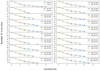 |
Fig. A.1. Total 1 ms count distribution for each of the 19 detectors (LE, ME, and 17 HE-NaI units): blue solid lines show the observed distribution, while the orange ones show the same distributions expected from a varying background model purely affected by Poisson noise. Bottom right panel: summed distribution of the HE units. |
Following the detailed inspection of these excesses, each of them is found in one individual detector at a time, so they are completely uncorrelated among different detectors and, as such, they are incompatible with what is expected from a plane wave. These spikes are therefore spurious and are likely to be mainly due to cosmic rays of a high atomic number, Z. They excite metastable states in the crystals, giving rise to a short-lived phosphorescence, which is nonetheless long enough to have the electronics detect several counts. This is probably the same effect as the one observed in the BeppoSAX Gamma-ray Burst Monitor during the initial months, before the lower-energy thresholds were finally increased (Feroci et al. 1997).
We tested this possibility in the case of HE data by selecting all the 1 ms bins with ≥6 counts and studying the distribution of these counts as a function of energy, considering three energy channels: 25 − 30, 30 − 40, and 40 − 80 keV. As a result, 80% of them are found to lie below 30 keV, while none of them pass the 40 keV threshold.
We further characterised the extra-Poissonian component in the HE case by modelling the observed total 1 ms count distribution, that is, the summed distribution of all 17 HE-NaI detectors, shown in the bottom-right panel of Fig. A.1. We found out that the overall distribution can reasonably be modelled as the sum of two independent Poisson processes with different constant rates. The dominant one has an average rate of 0.017 counts ms−1, while the other has a much larger rate (0.7 counts ms−1), but is active only for a limited amount of time and whose total exposure is just 2.6 × 10⁻⁴ times that of the dominant one. The result is shown in Fig. A.2. Therefore, we may consider the extra-Poissonian component to be attributed to the particle spikes that occasionally impact the detectors for a very limited fraction of the total observing time.
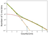 |
Fig. A.2. Total 1 ms count distribution of the 17 HE-NaI units (green points). This is modelled (green thick line) as the sum of two independent components: in addition to the one that accounts for ∼99% of the total counts with an average count rate of 0.017 counts ms−1 (blue points and orange solid line), there is an additional component (red solid line), which is responsible for the remaining 1% of counts, with an average count rate of 0.7 counts ms−1 and whose exposure is just 2.6 × 10⁻⁴ times the total net one. |
Appendix B: Trigger criteria of the Multi-Detector Search
The MDS conceived for the available data set of three instruments consists of three alternative criteria. Whenever the counts for a given time bin fulfil at least one of the three criteria, the corresponding event is promoted to the status of transient candidate. They mainly differ in the combinations of data sets to which they can be applied. Each of them is defined through a set of thresholds, expressed in Gaussian σ units as in Guidorzi et al. (2020), which must be exceeded by the counts recorded in a given time bin. These thresholds depend on the integration time, on the kind of detector, as well as on the number of detectors with available data. Table B.1 reports all of them.
Trigger criteria of the MDS.
All the parameters were tuned so as to end up with a relative small number of false positives (≲1) taking into account the multi-trials due to the total number of screened bins. As explained in Sect. 3.2, we started with a initial set based on the pure Poisson noise assumption. Next, in order to account for the impact of a small, but significant extra-Poissonian component due to the presence of occasional particle spikes, we refined them by means of Monte Carlo simulations. These were carried out by shuffling the observed data sets 100 times, thus preserving the properties of the count distributions of each individual detector. We then applied the MDS to these 100 statistically equivalent data sets to evaluate the false positive rate.
While the number of bins to be screened obviously decreases with increasing integration time, in considering Table B.1, it might appear puzzling to see the way the minimum number of HE units varies with integration time. These values were obtained taking into account the granularity of counts as a discrete and not a continuous distribution. This has an impact at the shortest integration times especially, for which the expected background counts per bin are ≪1. As a consequence, raising the threshold on counts by just one unit, implies a drastic change in the corresponding probability (see G20 for further explanations).
The three criteria are explained in more detail as follows:
-
This criterion demands that at least two instruments, one of which must be HE, fulfil the corresponding trigger condition. Given that HE consists of 17 independent units, the HE trigger condition includes a minimum number of HE units for which the corresponding threshold must be exceeded.
-
In this case, the combination of LE and ME is considered, regardless of HE. Compared with criterion 1, because of the lack of the multiple detector of different HE units, we must increase the thresholds on the LE and ME to avoid an excessively high rate of statistical flukes that may trigger it.
-
This criterion concerns HE data, regardless of the two softer instruments. Compared with criterion 1, the minimum number of HE units to be triggered is slightly higher, to compensate the lack of information from the other two instruments.
There are a couple of important points to make at this point: firstly, the time bins for which data is available from all instruments are screened through all three criteria. Secondly, the criteria are not strictly mutually exclusive, especially for bright events. For instance, a bright transient, for which filtered data from the three detectors are available, would trigger criterion 1 with all instruments, but could also trigger the other two criteria as well. Conversely, regardless of the event brightness, whenever only the filtered data from two instruments (or from HE alone) are available (for any reason; this is indeed the case for a non-negligible fraction of net exposure as reported in Table 1) criteria 2 and 3 come into play and make sure that the transient is not missed by the trigger logic. Furthermore, there are other possible cases for which the spectral properties of the event make it detectable only through specific criteria: when this is particularly soft, criterion 2 is more likely to trigger, whilst criterion 3 could work best when it is relatively dim and hard.
Given that the three criteria are not mutually exclusive, the expected false positive rate should be better estimated by applying them to simulated data sets that preserve the statistical properties of the count distributions of the individual detectors. This is the reason we opted for this choice. Our results are reported in Table 2: the number of expected false positives already accounts for the total number of screened time bins and includes all the three trigger criteria together.
All Tables
Number of candidates and expected false positives as a function of the integration time.
All Figures
|
Fig. 1. Detection probability for a flare as a function of duration, Δ t, fluence, F (left-hand y axis), and isotropic–equivalent released energy, Eiso (right-hand y axis) in the 1−100 keV energy band for two different energy spectra: an OTTB with kT = 50 keV (left) and a power-law with photon index, Γ = 2 (right). The different solid lines correspond to constant luminosity values. |
| In the text | |
|
Fig. A.1. Total 1 ms count distribution for each of the 19 detectors (LE, ME, and 17 HE-NaI units): blue solid lines show the observed distribution, while the orange ones show the same distributions expected from a varying background model purely affected by Poisson noise. Bottom right panel: summed distribution of the HE units. |
| In the text | |
|
Fig. A.2. Total 1 ms count distribution of the 17 HE-NaI units (green points). This is modelled (green thick line) as the sum of two independent components: in addition to the one that accounts for ∼99% of the total counts with an average count rate of 0.017 counts ms−1 (blue points and orange solid line), there is an additional component (red solid line), which is responsible for the remaining 1% of counts, with an average count rate of 0.7 counts ms−1 and whose exposure is just 2.6 × 10⁻⁴ times the total net one. |
| In the text | |
Current usage metrics show cumulative count of Article Views (full-text article views including HTML views, PDF and ePub downloads, according to the available data) and Abstracts Views on Vision4Press platform.
Data correspond to usage on the plateform after 2015. The current usage metrics is available 48-96 hours after online publication and is updated daily on week days.
Initial download of the metrics may take a while.