| Issue |
A&A
Volume 642, October 2020
|
|
|---|---|---|
| Article Number | A110 | |
| Number of page(s) | 10 | |
| Section | Planets and planetary systems | |
| DOI | https://doi.org/10.1051/0004-6361/202039066 | |
| Published online | 09 October 2020 | |
Four microlensing planets with faint-source stars identified in the 2016 and 2017 season data
1
Department of Physics, Chungbuk National University,
Cheongju
28644,
Republic of Korea
e-mail: This email address is being protected from spambots. You need JavaScript enabled to view it.
2
Warsaw University Observatory,
Al. Ujazdowskie 4,
00-478
Warszawa, Poland
3
Korea Astronomy and Space Science Institute,
Daejon
34055, Republic of Korea
4
Center for Astrophysics, Harvard & Smithsonian 60 Garden St.,
Cambridge,
MA
02138, USA
5
Department of Physics and Astronomy, University of Canterbury,
Private Bag 4800,
Christchurch
8020,
New Zealand
6
Korea University of Science and Technology,
217 Gajeong-ro,
Yuseong-gu,
Daejeon
34113, Republic of Korea
7
Max Planck Institute for Astronomy,
Königstuhl 17,
69117
Heidelberg, Germany
8
Department of Astronomy, The Ohio State University,
140 W. 18th Ave.,
Columbus,
OH
43210, USA
9
Department of Particle Physics and Astrophysics, Weizmann Institute of Science,
Rehovot
76100, Israel
10
Department of Astronomy and Tsinghua Centre for Astrophysics, Tsinghua University,
Beijing
100084,
PR China
11
School of Space Research, Kyung Hee University,
Yongin,
Kyeonggi
17104, Republic of Korea
12
Department of Astronomy & Space Science, Chungbuk National University,
Cheongju
28644, Republic of Korea
13
Department of Physics & Astronomy, Seoul National University,
Seoul
08826, Republic of Korea
14
Division of Physics, Mathematics, and Astronomy, California Institute of Technology,
Pasadena,
CA
91125, USA
15
Department of Physics, University of Warwick,
Gibbet Hill Road,
Coventry,
CV4 7AL, UK
Received:
30
July
2020
Accepted:
21
August
2020
Abstract
Aims. Microlensing planets occurring on faint-source stars can escape detection due to their weak signals. Occasionally, detections of such planets are not reported due to the difficulty of extracting high-profile scientific issues on the detected planets.
Methods. For the solid demographic census of microlensing planetary systems based on a complete sample, we investigate the microlensing data obtained in the 2016 and 2017 seasons to search for planetary signals in faint-source lensing events. From this investigation, we find four unpublished microlensing planets: KMT-2016-BLG-2364Lb, KMT-2016-BLG-2397Lb, OGLE-2017-BLG-0604Lb, and OGLE-2017-BLG-1375Lb.
Results. We analyze the observed lensing light curves and determine their lensing parameters. From Bayesian analyses conducted with the constraints from the measured parameters, it is found that the masses of the hosts and planets are in the ranges 0.50 ≲ Mhost∕M⊙≲ 0.85 and 0.5 ≲ Mp∕MJ ≲ 13.2, respectively, indicating that all planets are giant planets around host stars with subsolar masses. The lenses are located in the distance range of 3.8 ≲ DL∕kpc ≲ 6.4. It is found that the lenses of OGLE-2017-BLG-0604 and OGLE-2017-BLG-1375 are likely to be in the Galactic disk.
Key words: gravitational lensing: micro / planets and satellites: detection
© ESO 2020
1 Introduction
Although the probability of a source star being gravitationally lensed does not depend on the source brightness, the chances of detecting microlensing planets decreases as the source becomes fainter. This is because the signal-to-noise ratio (S/N) of the planetary signal in the lensing light curve of a faint-source event is low due to large photometric uncertainties, and thus if other conditions are the same, the planet detection efficiency of a faint-source event is lower than that of a bright source event (Jung et al. 2014). Even if faint-source planetary events are found despite their lower detection efficiency, they are occasionally left unpublished. The major reason for this is that it is difficult to extract high-profile scientific issues on the detected planets. Important scientific issues on microlensing planets are usually found when the physical parameters of the planetary lens systems, such as the mass M and distance DL, are well constrained. For the determinations of these parameters, it is required to simultaneously measure the angular Einstein radius, θE, and the microlens parallax, πE. The measurement of θE requires resolving caustic crossings in lensing light curves. For a faint-source event, the chance of measuring θE is low not only because of the low photometric precision, but also because a fainter source tends to be a smaller star and thus has a smaller angular source radius, θ*, and, as a result, a shorter duration caustic crossing; that is to say
 (1)
(1)
Here ψ denotes the caustic entrance angle of the source star. The measurement of πE calls for the detection of subtle deviations in the lensing light curve induced by microlens-parallax effects (Gould 1992), but this measurement is usually difficult for faint-source events due to the low photometric precision.
Reporting discovered planets is important because otherwise they would not be included in the planet sample that is used for the statistical investigation of planet properties and frequency, for example by Gould et al. (2010b), Sumi et al. (2010), and Suzuki et al. (2018). As of the time of writing this article, there are 119 microlensing planets in 108 planetary systems1. However, the solid characterization of planet properties based on the demographic census of microlensing planets requires publishing the discoveries of all microlensing planets, including those with faint sources.
In this paper, we report four planetary systems found from the investigation of faint-source microlensing events discovered in the 2016 and 2017 seasons. For the presentation of the work, we organize the paper as follows. In Sect. 2, we state the selection procedure of the analyzed planetary lensing events and the data used for the analyses. In Sect. 3, we describe the analysis method commonly applied to the events and discuss the results from the analyses of the individual events. In Sect. 4, we characterize the source stars of the events by measuring their color and brightness, and we estimate θE of the events with measured finite-source effects. In Sect. 5, we estimate the physical lens parameters by applying the constraints from the available observables related to the parameters. We summarize the results and conclude in Sect. 6.
2 Event selection and data
Planetary microlensing signals can escape detection in the myriad of data obtained by lensing surveys. Updated microlensing data are available in the public domain so that anomalies of various types in lensing light curves can be found for events in progress and trigger decisions to conduct follow-up observations, if necessary, for dense coverage of anomalies, for example the OGLE Early Warning System (Udalski et al. 1994), MOA Alert System (Bond et al. 2001), and KMTNet Alert Finder System (Kim et al. 2018b). To make this process work successfully, several modelers (V. Bozza, Y. Hirao, D. Bennett, M. Albrow, Y. K. Jung, Y. H. Ryu, A. Cassan, and W. Zang) investigate the light curves of lensing events in real time, find anomalous events, and circulate possible interpretations of the anomalies to researchers in the microlensing community. Despite these efforts, some planets may escape detection for various reasons. One of these reasons is the large number of lensing events. During the first generation surveys, for example the MACHO (Alcock et al. 1995) and OGLE-I (Udalski et al. 1992) surveys, several dozen lensing events were detected annually, and thus individual events could be thoroughly investigated. However, the number of event detections has dramatically increased with the enhanced cadence of lensing surveys, for example the OGLE-IV (Udalski et al. 2015), MOA (Bond et al. 2001), and KMTNet (Kim et al. 2016) surveys; they use globally distributed multiple telescopes equipped with large-format cameras yielding very wide fields of view, and the current lensing surveys annually detect about 3000 events. Among these events, some planetary lensing events may not be noticed, especially those with weak planetary signals hidden in the scatter or noise of the data.
Considering the possibility of missing planets, we thoroughly investigated the microlensing data of the OGLE and KMTNet surveys obtained in the 2016 and 2017 seasons, paying special attention to events that occurred on faint-source stars. From this investigation, we find one planetary event that was not previously known. This event is KMT-2016-BLG-2364. We also investigate events with known planets, for which the findings have not been published or there is no plan to publish on the individual event basis. There exist three such events: KMT-2016-BLG-2397, OGLE-2017-BLG-0604, and OGLE-2017-BLG-1375. In this work, we present a detailed analysis of these four planetary events.
The analyzed planetary lensing events are located toward the Galactic bulge field. The positions of the individual events, both in equatorial and Galactic coordinates, are listed in Table 1. All these events occurred in the fields that were commonly observed by both surveys. The event OGLE-2017-BLG-1375/KMT-2017-BLG-0078, hereafter referred to as OGLE-2017-BLG-1375 as a representative name of the event according to the chronological order of the event discovery, was found by both surveys. However, the other events were detected by only a single survey and escaped detection by the other: The two events KMT-2016-BLG-2364 and KMT-2016-BLG-2397 were found only by the KMTNet survey, and the event OGLE-2017-BLG-0604 was found solely by the OGLE survey. Although these events were detected by a single survey, we use data from both surveys in our analysis by conducting post-event photometry of the events.
Observations of the events by the OGLE survey were conducted using the 1.3 m telescope of the Las Campanas Observatory in Chile. The telescope is equipped with a camera yielding a 1.4 deg2 field of view. The KMTNet survey used three identical 1.6 m telescopes located at the Siding Spring Observatoryin Australia (KMTA), the Cerro Tololo Interamerican Observatory in Chile (KMTC), and the South African Astronomical Observatory in South Africa (KMTS). Hereafter, we refer to the individual KMTNet telescopes as KMTA, KMTC, and KMTS. Each KMTNet telescope is equipped with a camera providing a 4 deg2 field of view. For both surveys, observations were mainly carried out in the I band, and V -band observationswere conducted for a subset of images to measure the source color. We give a detailed description of the procedure of the source color measurement in Sect. 4.
Photometry of the events was carried out using the software pipelines developed by the individual survey groups: Udalski (2003) using the DIA technique of Woźniak (2000) for the OGLE survey, and Albrow et al. (2009) for the KMTNet survey. Both pipelines are based on the difference imaging method (Tomaney & Crotts 1996; Alard & Lupton 1998), which is optimized for dense field photometry. For a subset of the KMTC I- and V -band images, we conducted additional photometry using the pyDIA software (Albrow 2017) for the source color measurement. For the data used in the analysis, we readjusted the error bars of the data so that the cumulative χ2 distribution with respect to the lensing magnification became linear and χ2 per degree of freedom for each data set became unity (Yee et al. 2012).
Coordinates of events.
3 Analyses
The modeling of each lensing event is carried out by searching for the parameters that best explain the observed light curve. The light curves of the analyzed events share the common characteristics that the events are produced by a binary lens and a single source (2L1S) with discontinuous caustic-involved features. The light curves of such 2L1S events are described by seven lensing parameters. The first three of these parameters are those of a single-lens single-source (1L1S) event, including (t0, u0, tE), which denote the time of the closest lens approach to the source, the impact parameter of the lens-source encounter (in units of θE), and the event timescale, respectively. The next three parameters are related to the binarity of the lens, and these parameters include (s, q, α), which indicate the projected binary separation (in units of θE), the mass ratio between the lens components M1 and M2, and the incidence angle of the source trajectory as measured from the M1 –M2 axis, respectively. The last parameter is the normalized source radius ρ, which is included in the modeling because the light curves of all analyzed events exhibit discontinuous features that are likely to be involved with source stars’ caustic crossings, during which the lensing light curve is affected by finite-source effects.
The procedure of modeling commonly applied to the analysis is as follows. In the first-round modeling, we searched for the binary lensing parameters s and q using a grid-search approach, while the other lensing parameters were found using a downhill method, which is based on the Markov chain Monte Carlo (MCMC) algorithm. From the Δχ2 map in the s–q plane constructed from this round of modeling, we identified local minima. In the second-round modeling, we inspected the individual local minima and refined the lensing parameters by releasing all parameters, including s and q, as free parameters. We then compared the χ2 values of the local solutions, not only to find a global solution but also to find degenerate solutions if they exist. In the following subsections, we present details of the analysis applied to the individual events and the results from the analysis.
3.1 KMT-2016-BLG-2364
KMT-2016-BLG-2364 is a lensing event for which the existence of a very low-mass companion to the lens was not known during the season of the event and was found from the post-season inspection of the 2016 season data (Kim et al. 2018a). Figure 1 shows the lensing light curve of the event. The dotted curve superposed on the data points represents the 1L1S model. The planet-induced anomalies appear in the two very localized regions around HJD′ ≡ HJD − 2 450 000 ~ 7600 and ~ 7607, for which the zoomed-in views are shown in the upper left and upper right panels, respectively. It was difficult to notice the anomalies of the light curve constructed with the online KMTNet data at a casual glance; the former anomaly (at HJD′ ~ 7600) was covered by only two data points and the latter anomaly (at HJD′ ~ 7607) was hidden in the scatter and noise of the online data processed by the automated photometry pipeline. We inspected the event to check whether the two points at HJD′ = 7600.72 and 7600.85 were real by first re-reducing the data for optimal photometry and then conducting 2L1S modeling. This procedure not only confirmed the reality of the former anomaly but also enabled us to unexpectedly find the latter anomaly. The anomalous features are additionally confirmed with the addition of the OGLE data processed after the analysis based on the KMTNet data.
From modeling the light curve, we find that the anomalies are produced by a planetary companion to the primary lens with (s, q)~ (1.17, 7.6 × 10⁻³). The model curveof the solution, the solid curve plotted over the data points, is presented in Fig. 1, and the lensing parameters of the solution are listed in Table 2. We find that the presented solution is unique without any degeneracy due to the special lens system configuration (see below) producing the anomalies at two remotely separated regions. Also listed in Table 2 are the flux values and magnitudes of the source at the baseline, fs and Is. The flux is on an I = 18 scale (i.e., f = 10−0.4(I−18)). It is found that the source of the event is very faint, with an apparent magnitude of Is ~ 21.9.
The configuration of the lens system is shown in Fig. 2, in which the trajectory of the source (line with an arrow) relative to the positions of the lens components (marked by blue dots) and the resulting lensing caustic (red cusp-like closed figure) are presented. The lens system induces a single large caustic with six cusps (i.e., resonant caustic) due to the closeness of the binary separation to unity. According to the solution, the anomalies at HJD′ ~ 7600 and ~ 7607 were produced when the source passed the upper left and upper right tips of the caustic, respectively. We checked the feasibility of measuring the microlens parallax πE by conducting additional modeling. This modeling required including the extra parameters πE,N and πE,E, which represent the north and east components of πE, respectively. From this, itis found that πE cannot be securely measured, mostly due to the relatively large uncertainties of the data caused by the faintness of the source together with the relatively short event timescale, tE ~21 days. Although both anomalies are captured, the caustic crossings are poorly resolved, and this makes it difficult to constrain the normalized source radius ρ. This is shown in the Δχ2 distribution of points in the MCMC chain on the q–ρ plane presented in Fig. 3. It is found that the observed light curve is consistent with a point-source model, although the upper limit is constrained to be ρ ≲ 0.003 as measured at the 3σ level.
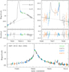 |
Fig. 1 Light curve of KMT-2016-BLG-2364. The dotted and solid curves superposed on the data points are the lL1S and 2L1S models, respectively. The lensing parameters of the 2L1S model are presented in Table 2. Upper panels: enlarged views of the regions around HJD′ ~ 7601 (left panel) and ~7607 (right panel) when the planet-induced anomalies occur. The lens system configuration of the 2L1S solution is presented in Fig. 2. |
Lensing parameters of KMT-2016-BLG-2364.
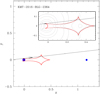 |
Fig. 2 Configuration of the KMT-2016-BLG-2364 lens system. The line with an arrow denotes the source trajectory with respect to the lens components that are marked by filled blue dots. The cusp-like closed figure drawn in red represents the caustic. The inset shows the enlargement of the central magnification region. The gray curves around the caustic represent equi-magnification contours. Lengths are normalized to the angular Einstein radius corresponding to the total lens mass. |
3.2 KMT-2016-BLG-2397
The event KMT-2016-BLG-2397 was found by the KMTNet survey, and the OGLE data were recovered from the post-event photometry for the lensing source identified by the KMTNet survey. The anomaly, which occurred at HJD′ ~ 7550.4 near the peak, lasted for ~1.5 days. The planetary origin of the anomaly was known by several modelers of the KMTNet group from the analyses of the online data conducted during the 2016 season, but no extended analysis based on optimized photometric data had been presented until this work.
The light curve of KMT-2016-BLG-2397 is shown in Fig. 4, in which the enlarged view around the anomaly is presented inthe upper panel. The combination of the six KMTC data points plus two OGLE points in the anomaly region display a “U”-shape pattern, which is a characteristic pattern that appears during the passage of a source inside a caustic, indicating that the anomaly is produced by caustic crossings. Modeling the light curve yields two degenerate solutions resulting from the close–wide degeneracy (Griest & Safizadeh 1998; Dominik 1999). The binary parameters are (s, q)~ (0.93, 3.72 × 10⁻³) and ~ (1.15, 3.95 × 10⁻³) for the close (s < 1.0) and wide (s > 1.0) solutions, respectively, indicating that the anomaly is generated by a planetary companion to the primary lens located near the Einsteinring of the primary. The degeneracy between the close and wide solutions is very severe, and the χ2 difference between the two degenerate models is merely Δχ2 = 0.5. The lensing parameters of the two solutions are listed in Table 3 together with χ2 values of the fits.
The lens system configuration of the event is displayed in Fig. 5. The upper and lower panels show the configurations for the close and wide solutions, respectively, and the inset in each panel shows the enlarged view of the central magnification region. As in the case of KMT-2016-BLG-2364, the lens system forms a single large resonant caustic because the binary separation is similar to θE (i.e., s ~ 1). For both close and wide solutions, the source trajectory passes the planet side of the caustic, producing an anomaly characterized by two spikes and a U-shape trough region between the spikes.
The light curve of KMT-2016-BLG-2397 shares many characteristics in common with those of KMT-2016-BLG-2364. First, the source star of the event is very faint, with a baseline magnitude of I ~ 21.7. Second, the caustic crossings are not well resolved, and this makes it difficult to constrain the normalized source radius ρ, although the upper limit is set to be ρ ≲ 0.0015. The Δχ2 distribution on the q–ρ plane is presented in Fig. 3. Third, due to the substantial uncertainty of the photometric data caused by the faintness of the source, the microlens parallax πE cannot be securely determined despite the relatively long timescale of the event, which is tE ~ 53 days for the close solution andtE ~ 58 days for the wide solution.
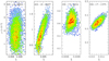 |
Fig. 3 Δχ2 distributions of points in the MCMC chain on the q–ρ plane for the individual lensing events. The colors of the data points indicate regions with ≤ 1σ (red), ≤ 2σ (yellow), ≤3σ (green), ≤4σ (cyan), and ≤5σ (blue). |
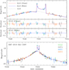 |
Fig. 4 Lensing light curve of KMT-2016-BLG-2397. The dotted and solid curves are the 1L1S and 2L1S models, respectively. The enlarged view of the anomaly region is shown in the top panel. Second and third panels: residuals from the “close” and “wide” 2L1S solutions, for which the corresponding lensing parameters are presented in Table 3 and the lens system configurations are shown in Fig. 5. |
Lensing parameters of KMT-2016-BLG-2397.
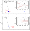 |
Fig. 5 Configuration of the lens system for the lensing event KMT-2016-BLG-2397. Upper and lower panels: those of the close (s < 1.0) and wide (s > 1.0) solutions, respectively. Notations are same as those in Fig. 3. |
3.3 OGLE-2017-BLG-0604
The lensing event OGLE-2017-BLG-0604 was found by the OGLE survey. The source star was very faint, with a baseline magnitude of I ~ 21.6. Together with the low magnification, with a peak magnification Apeak ~ 3.3, the event was not detected by the event-finder system of the KMTNet survey (Kim et al. 2018a). The existence of a possible short-term anomaly in the OGLE light curve was noticed by KMTNet modelers. Realizing that the event is located in the KMTNet field, we conducted photometry for the KMTNet images at the location of the source using the finding chart provided by the OGLE survey and recovered the KMTNet light curve of the event. It is found that the additional KMTNet data are crucial in finding a unique solution for the event. More detailed discussions are given below.
The light curve of OGLE-2017-BLG-0604 is displayed in Fig. 6. The upper panel shows the zoomed-in view of the anomaly region during 7868 ≲HJD′≲ 7873. The anomaly is composed of two parts: the brief bump centered at HJD′ ~ 7869.6 (covered mainly by the KMTS data set) and the caustic-crossing features between 7870.6 ≲HJD′≲ 7872.0 (covered by all data sets). The first part of the anomaly is not obvious in the OGLE data, and the modeling based on only the OGLE data yields several possible solutions caused by accidental degeneracies. However, modeling with the use of the additional KMTNet data, which clearly shows the first anomaly, yields a unique solution, excluding the other solutions found from the modeling without the KMTNet data. This indicates that the data covering the first part of the anomaly are crucial for the accurate characterization of the lens system.
The lensing parameters of the best-fit solution are listed in Table 4, and the lens system configuration corresponding to the solution is shown in Fig. 7. The estimated binary parameters are (s, q) ~ (1.20, 0.70 × 10⁻³), indicating that the anomalies are produced by a planetary companion to the lens. The planet induces two sets of caustics, one of which is located near the location of the primary (central caustic) and the other is located away from the host (planetary caustic), toward the direction of the planet with a separation of s − 1∕s ~ 0.37 (Griest & Safizadeh 1998; Han 2006). The anomaly in the lensing light curve was produced by the source star’s approach and crossings over the planetary caustic. Before the caustic crossings, which produced the major caustic-crossing feature in the lensing light curve, the source approached the upper cusp of the caustic, and this produced the first part of the anomaly at HJD′ ~ 7869.6. This can be seen in the enlarged view of the planetary caustic and the source trajectory shown in the upper inset of Fig. 7. The lower two insets show the configurations of the lens systems for the two degenerate solutions, with (s, q) ~ (0.90, 0.027) and ~ (1.08, 0.028), obtained from the modeling not using the KMTNet data. These solutions describe almost equally well the second part of the anomaly as the presented solution, but cannot explain the first part of the anomaly. The coverage of the first part of the anomaly also enables us to measure the normalized source radius of ρ ~ 0.60 × 10⁻³. Figure 3 shows the Δχ2 distribution of MCMC points on the q–ρ plane. However, the microlens parallax cannot be determined due to the substantial photometric uncertainty of the data caused by the faintness of the source star.
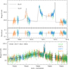 |
Fig. 6 Light curve of OGLE-2017-BLG-0604. The enlarged view around the anomaly is presented in the upper panel. Notations are same as those in Fig. 1. The lensing parameters of the solutions are presented in Table 4, and the corresponding lens system configuration is shown in Fig. 7. |
Lensing parameters of OGLE-2017-BLG-0604.
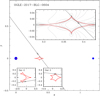 |
Fig. 7 Configuration of the OGLE-2017-BLG-0604 lens system. Upper right inset: close-up view of the planetary caustic and the source trajectory. Two lower left insets: configurations of the two degenerate solutions obtained from modeling with only the OGLE data, which do not cover the first part of the anomaly at HJD′ ~ 7869.6. These degenerate solutions cannot explain the first part of the anomaly, although they describe the second part of the anomaly as the presented solution almost equally well. |
3.4 OGLE-2017-BLG-1375
The event OGLE-2017-BLG-1375 was first found by the Early Warning System (Udalski et al. 1994) of the OGLE survey on July 20, 2017, HJD′ ~ 7954. Later, the event was independently found by the KMTNet Event Finder System (Kim et al. 2018a) and it was designated as KMT-2017-BLG-0078. The source is a faint star with an I-band magnitude of Is ~ 21.6.
The light curve of the lensing event is displayed in Fig. 8. It shows an obvious caustic-crossing feature, in which the spikes at HJD′ ~ 7966.43 and ~7970.95 are caused by the caustic entrance and exit of the source star, respectively. The individual caustic crossings were covered by the KMTS (for the caustic entrance) and KMTA (for the caustic exit) data sets. This can be seen in the upper panels, which show the enlarged views of the caustic-crossing parts of the light curve. The obvious anomaly feature led to real-time modeling of the event based on the online data at the time of the anomaly by several KMTNet modelers, but no result from a detailed analysis had been reported before this work.
Analysis using the data obtained from optimized photometry indicates that the event is produced by a binary lens with a low-mass companion. Interpreting the event is subject to a close–wide degeneracy, and the estimated binary parameters are (s, q) ~ (0.84, 0.013) for the close solution and(s, q) ~ (1.27, 0.015) for the wide solution. The lensing parameters for both solutions based on the rectilinear (linear motion without acceleration) relative lens-source motion (“standard solution”) are listed in Table 5. Because the caustic crossings are resolved, the normalized source radius, ρ ~ (0.33−0.34) × 10−3, is well constrained, as shown in the Δχ2 distribution of MCMC points in Fig. 3. Figure 9 shows the lens system configurations for the close (upper panel) and wide (lower panel) binary solutions. The inset for each configuration shows the close-up view of the central magnification region, through which the source passed. According to both solutions, the anomaly was produced by the source passage over the planet-side central caustic.
Because the event timescale, tE ≳ 100 days, is considerably long, we checked the feasibility of measuring the microlens parallax by conducting additional modeling of the light curve considering the microlens-parallax effect. Because it is known that the microlens-parallax effect can be correlated with the effect of the lens orbital motion (Batista et al. 2011; Skowron et al. 2011; Han et al. 2016), we additionally considered the orbital motion of the lens in the modeling. Considering the lens orbital motion requires the inclusion of two additional parameters, d s∕dt and d α∕dt, which represent the change rates of the binary separation and the source trajectory angle, respectively. We also checked the “ecliptic degeneracy” between the pair of solutions with u0 > 0 and u0 < 0 caused by the mirror symmetry of the lens system configuration with respect to the binary axis (Skowron et al. 2011). The lensing parameters of the two solutions subject to this degeneracy are roughly related by (u0, α, πE,N, dα) ↔−(u0, α, πE,N, dα).
Figure 10 shows the distributions of points in the MCMC chain on the πE,E–πE,N parameter plane for the close (with u0 < 0, left panel) and wide (with u0 > 0, right panel)solutions. We note that the corresponding solutions with opposite signs of u0 exhibit similar distributions. The distributions show that πE,E is relatively well constrained, but the uncertainty of πE,N is substantial; this results in a large uncertainty of  . The uncertainties of the lens-orbital parameters (i.e., ds∕dt and dα∕dt) are also very large. As a result, the improvement of the fit by the higher-order effects is minor, with Δχ2 < 8 for all solutions. In Table 5, we list the lensing parameters estimated by considering the higher-order effects. We note that the lens-orbital parameters are not listed in the table because they are poorly constrained. It is found that the basic lensing parameters (t0, u0, tE, s, q, α) vary little from those of the standard solution with the consideration of the higher-order effects.
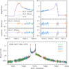 |
Fig. 8 Light curve of OGLE-2017-BLG-1375. Upper left and upper right panels: close-up views of the caustic entrance and exit of the source, respectively. For each of the upper panels, we present two sets of residuals from the close and wide binary solutions. The lensing parameters of the solutions are presented in Table 5, and the lens system configuration is shown in Fig. 9. |
Lensing parameters of OGLE-2017-BLG-1375.
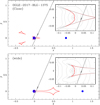 |
Fig. 9 Lens configuration of the event OGLE-2017-BLG-1375. Upper and lower panels: configurations for the close and wide solutions, respectively. Notations are same as those in Fig. 2. |
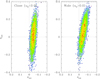 |
Fig. 10 Distribution of points in the MCMC chain on the πE,E–πE,N parameter plane for OGLE-2017-BLG-1375. Left and right panels: close (with u0 < 0) and wide (with u0 > 0) binary solutions, respectively. The color coding is set to denote points with < 1σ (red), <2σ (yellow), <3σ (green), <4σ (cyan), and <5σ (blue). The dotted crosshair represents the lines with (πE,E, πE,N) = (0.0, 0.0). |
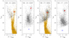 |
Fig. 11 Positions of the source (marked by an empty blue dot with error bars) and RGC centroid (red dot) in the instrumental color-magnitude diagrams. For the events KMT-2016-BLG-2397 and OGLE-2017-BLG-1375, the CMDs are constructed using the pyDIA photometry of the KMTC data set. For KMT-2016-BLG-2364 and OGLE-2017-BLG-0604, the CMDs are based on the combinations of the OGLE (gray points) and HST (yellow points) data sets. |
4 Source stars and Einstein radius
We checked the feasibility of measuring the angular Einstein radii of the events. The measurement of θE requires the characterization the source color, V −I, from which the angular source radius θ* is estimated and the angular Einstein radius is determined by θE = θ*∕ρ. We were able to measure the source colors for KMT-2016-BLG-2397 and OGLE-2017-BLG-1375 using the usual method from the regression of V - and I-band magnitudes of data with the change of the lensing magnification (Gould et al. 2010a). However, the source colors for KMT-2016-BLG-2364 and OGLE-2017-BLG-0604 cannot be measured using this method because the V -band magnitudes of the events cannot be securely measured due to the faintness of the source together with the severe V -band extinction of the fields, although the I-band magnitudes are measured. For the last two events, we estimated the source color using the Hubble Space Telescope (HST) color-magnitude diagram (CMD; Holtzman, et al. 1998). In this method, the ground-based CMD was aligned with the HST CMD using the red giant clump (RGC) centroids in the individual CMDs; we then estimated the range of the source color as the width (standard deviation) of the main-sequence branch in the HST CMD for a given I-band brightness difference between the source and RGC centroid (Bennett et al. 2008; Shin et al. 2019). Besides the V − I color, estimating θE also requires measuring the normalized source radius ρ. This was done for the events OGLE-2017-BLG-0604 and OGLE-2017-BLG-1375. For the events KMT-2016-BLG-2364 and KMT-2016-BLG-2397, on the other hand, we could only place upper limits on ρ, and thus set the lower limits of θE for these two events.
For the θ* estimation, we used the method in Yoo et al. (2004). According to this method, θ* is estimatedbased on the extinction corrected (de-reddened) source color and magnitude,  , which were estimated using the RGC centroid as a reference, for which its de-reddened color and magnitude,
  , are known. Following the procedure of the method, we first located the source and RGC centroid in the instrumental CMD of stars in the vicinity of the source; measured the offsets in color, Δ(V−I), and brightness, ΔI, of the source from the RGC centroid; and then estimated the de-reddened source color and magnitude by
 (2)
(2)
In this process, we used the reference values of  estimated by Bensby et al. (2013) and Nataf et al. (2013).
Figure 11 shows the locations of the source and RGC centroid in the ground-based instrumental CMDs of stars (gray dots) around the source stars of the individual events. For the events KMT-2016-BLG-2364 and OGLE-2017-BLG-0604, for which the V -band source colors cannot be measured, we additionally present the HST CMDs (yellow dots), from which the source colors are derived. In Table 6, we list the values of the instrumental color and brightness for the source stars, (V −I, I), and the RGC centroids,  , and the de-reddened color and magnitude of the source star,
  , for the individual events. The measured source colors and magnitudes indicate that the source stars have spectral types later than G2.
We estimated θ* based on the measured source colors and magnitudes. For this, we first converted V − I into V − K using the color–color relation in Bessell & Brett (1988) and then estimated θ* using the (V −K)∕θ* relation in Kervella et al. (2004). We determined θE from the estimated θ* by using the relation θE = θ*∕ρ and estimated the relative lens-source proper motion from the combination of θE and tE by μ = θE∕tE. We summarize the estimated values of θ*, θE, and μ in Table 6. We note that the measured θE values for the events OGLE-2017-BLG-0604 and OGLE-2017-BLG-1375 are about two times bigger than the value of a typical lensing event produced by a lens located roughly halfway between the source and lens, and this suggests that the lenses for these events are likely to be located close to the observer.
5 Physical lens parameters
The lensing observables that can constrain the physical lens parameters of the mass and distance are tE, θE, and πE. The event timescale is routinely measurable for most events, but θE and πE are measurable only for events satisfying specific conditions. If all these observables are measured, the physical lens parameters are uniquely determined by
 (3)
(3)
where κ = 4G∕(c2au), πS = au∕DS, and DS denotes the source distance. For the analyzed events in this work, the availability of the observables varies depending on the events. The event timescales are measured for all events. The angular Einstein radii are measured for OGLE-2017-BLG-0604 and OGLE-2017-BLG-1375, but only the lower limits are set for KMT-2016-BLG-2364 and KMT-2016-BLG-2397. The microlens parallax is measured only for OGLE-2017-BLG-1375, although the uncertainty of the measured πE is fairly large. We summarize the available observables for the individual events in Table 7. Considering the incompleteness of the information for the unique determinations of M and DL, we estimated the physical lens parameters by conducting Bayesian analyses with the constraint provided by the available observables of the individual events and using the priors of the lens mass function, physical Galactic models, and dynamical Galactic models.
A Bayesian analysis was carried out by producing a large number (4 × 10⁷) of artificial lensing events from a Monte Carlo simulation using the priors. The priors of the Galactic model are based on the modified version of the Han & Gould (2003) model for the physical matter density distribution and on the Han & Gould (1995) model for the distribution of the relative lens-source transverse speed. For the mass function, weused the Zhang et al. (2019) model for stellar and brown-dwarf lenses and the Gould (2000) model for remnant lenses (i.e., white dwarfs, neutron stars, and black holes). More details on the models are available in Sect. 5 of Han et al. (2020). With the produced events, we then obtained the posteriors for M and DL by constructingthe probability distributions of events by applying the constraints available for the individual events. Although θE values are not uniquely measured for KMT-2016-BLG-2364 and KMT-2016-BLG-2397, we applied the constraint of their lower values. For OGLE-2017-BLG-1375, we applied a two-dimensional constraint of πE (i.e., (πE,N, πE,E)). With the constructed probability distributions, we then chose representative values of the physical parameters as the median of the distributions and estimated the uncertainties of the parameters as the 16 and 84% ranges of the distributions.
In Fig. 12, we present the posteriors of the host mass (left panels), Mhost, and the distanceto the lens (right panels) for the individual events. The estimated masses of the lens components (Mhost and Mp= qMhost), distance (DL), and projected planet-host separation (a⊥ = sDLθE) are summarized in Table 8. The masses of the hosts and planets are in the ranges 0.50≲ Mhost∕M⊙≲ 0.85 and 0.5 ≲ Mp∕MJ ≲ 13, respectively,indicating that all planetary systems are composed of giant planets and host stars with subsolar masses. It should be noted that the lower mass component of OGLE-2017-BLG-1375L lies at around the boundary between planets and brown dwarfs, that is to say ~ 13 MJ (Boss et al. 2007). The lenses are located in the distance range of 3.8 ≲ DL∕kpc ≲ 6.4. We note that the lenses of OGLE-2017-BLG-0604 and OGLE-2017-BLG-1375 (both with DL ~ 4 kpc) are likely to be in the Galactic disk.
We note that three of the four planetary hosts analyzed in this paper can almost certainly be resolved by adaptive optics (AO) observations on next-generation “30m” telescopes at AO first light (roughly 2030). That is, according to Fig. 12, each host of the four lens systems has only a tiny probability of being nonluminous. Furthermore, with exception of KMT-2016-BLG-2397, all lensing events have relative lens-source proper motions μ ≳ 3 mas yr−1. Hence, in 2030 they will be separated from the source by Δθ ≳ 40 mas. It is very likely that KMT-2016-BLG-2397 can also be resolved, unless it is extremely close to the limit that we report in Table 6. Given that tE is well measured for all four events, such a proper-motion measurement will immediately yield a θE measurement for the two events that do not already have one, as well as a more precise θE measurement for the other two. Combined with the K-band source flux measurement from the AO observations themselves, this will yield good estimates of the lens mass and distance. In the case of OGLE-2017-BLG-1375, the one-dimensional parallax measurement will enable even more precise determinations (Gould 2014).
Source color, magnitude, angular radius, Einstein radius, and proper motion.
Availability of lensing observables.
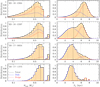 |
Fig. 12 Posteriors of the host mass Mhost (left panels) and the distance DL (right panels) to the lens for the individual events obtained by Bayesian analyses. In each panel, the blue and red distributions represent the contributions by the disk and bulge lens populations, respectively, and the black distribution is the sum of the contributions by two lens populations. The solidvertical line indicates the median value, and the two dotted vertical lines represent the 1σ range of the distribution. |
Physical lens parameters.
6 Summary and conclusion
For a solid demographic census of microlensing planetary systems based on a more complete sample, we investigated microlensing data in the 2016 and 2017 seasons obtained by the KMTNet and OGLE surveys to search for missing or unpublished planetary microlensing events. From this investigation, we found four planetary events: KMT-2016-BLG-2364, KMT-2016-BLG-2397, OGLE-2017-BLG-0604, and OGLE-2017-BLG-1375. It was found that the events share a common characteristic: the sources were faint stars. We presented the detailed procedure of modeling the observed light curves conducted to determine lensing parameters and presented models for the individual lensing events. We then carried out Bayesian analyses for the individual events using the available observables that could constrain the physical lens parameters of the mass and distance. From these analyses, it was found that the masses of the hosts and planets were in the ranges 0.50≲ Mhost∕M⊙≲ 0.85 and 0.5 ≲ Mp∕MJ ≲ 13, respectively, indicating that all planets were giant planets around host stars with subsolar masses. It was estimated that the distances to the lenses were in the range of 3.8 ≲ DL∕kpc ≲ 6.4. It was found that the lenses of OGLE-2017-BLG-0604 and OGLE-2017-BLG-1375 were likely to be in the Galactic disk.
Acknowledgements
Work by C.H. was supported by the grants of National Research Foundation of Korea (2017R1A4A1015178 and 2020R1A4A2002885). Work by A.G. was supported by JPL grant 1500811. This research has made use of the KMTNet system operated by the Korea Astronomy and Space Science Institute (KASI) and the data were obtained at three host sites of CTIO in Chile, SAAO in South Africa, and SSO in Australia. The OGLE project has received funding from the National Science Centre, Poland, grant MAESTRO 2014/14/A/ST9/00121 to AU.
References
- Alard, C., & Lupton, R. H. 1998, ApJ, 503, 325 [NASA ADS] [CrossRef] [Google Scholar]
- Albrow, M. 2017, http://doi.org/10.5281/zenodo.268049 [Google Scholar]
- Albrow, M., Horne, K., Bramich, D. M., et al. 2009, MNRAS, 397, 2099 [NASA ADS] [CrossRef] [Google Scholar]
- Alcock, C., Allsman, R. A., Axelrod, T. S., et al. 1995, ApJ, 445, 133 [NASA ADS] [CrossRef] [Google Scholar]
- Batista, V., Gould, A., Dieters, S., et al. 2011, A&A, 529, A102 [NASA ADS] [CrossRef] [EDP Sciences] [Google Scholar]
- Bennett, D. P., Bond, I. A., Udalski, A., et al. 2008, ApJ, 684, 663 [NASA ADS] [CrossRef] [Google Scholar]
- Bensby, T., Yee, J. C., Feltzing, S., et al. 2013, A&A, 549, A147 [NASA ADS] [CrossRef] [EDP Sciences] [Google Scholar]
- Bessell, M. S., & Brett, J. M. 1988, PASP, 100, 1134 [NASA ADS] [CrossRef] [Google Scholar]
- Bond, I. A., Abe, F., Dodd, R. J., et al. 2001, MNRAS, 327, 868 [Google Scholar]
- Boss, A. P., Butler, R. P., Hubbard, W. B., et al. 2007, Transactions of the International Astronomical Union, Series A, ed. O. Engvold (Cambridge: Cambridge University Press), 26, 183 [Google Scholar]
- Dominik, M. 1999, A&A, 349, 108 [NASA ADS] [Google Scholar]
- Gould, A. 1992, ApJ, 392, 442 [NASA ADS] [CrossRef] [EDP Sciences] [Google Scholar]
- Gould, A. 2000, ApJ, 535, 928 [NASA ADS] [CrossRef] [Google Scholar]
- Gould, A. 2014, J. Korean Astron. Soc., 47, 153 [CrossRef] [Google Scholar]
- Gould, A., Dong, S., Bennett, D. P., et al. 2010a, ApJ, 710, 1800 [NASA ADS] [CrossRef] [Google Scholar]
- Gould, A., Dong, S., Gaudi, B. S., et al. 2010b, ApJ, 720, 1073 [NASA ADS] [CrossRef] [Google Scholar]
- Griest, K., & Safizadeh, N. 1998, ApJ, 500, 37 [NASA ADS] [CrossRef] [Google Scholar]
- Han, C. 2006, ApJ, 638, 1080 [NASA ADS] [CrossRef] [Google Scholar]
- Han, C., & Gould, A. 1995, ApJ, 447, 53 [NASA ADS] [CrossRef] [Google Scholar]
- Han, C., & Gould, A. 2003, ApJ, 592, 172 [NASA ADS] [CrossRef] [Google Scholar]
- Han, C., Udalski, A., Lee, C.-U., et al. 2016, ApJ, 827, 11 [CrossRef] [Google Scholar]
- Han, C., Shin, I.-G., Jung, Y. K., et al. 2020, A&A, 641, A105 [CrossRef] [EDP Sciences] [Google Scholar]
- Holtzman, J. A., Watson, A. M., Baum, W. A., et al. 1998, AJ, 115, 1946 [NASA ADS] [CrossRef] [Google Scholar]
- Jung, Y. K., Park, H., Han, C., et al. 2014, ApJ, 786, 85 [CrossRef] [Google Scholar]
- Kervella, P., Thévenin, F., Di Folco, E., & Ségransan, D. 2004, A&A, 426, 29 [Google Scholar]
- Kim, S.-L., Lee, C.-U., Park, B.-G., et al. 2016, J. Korean Astron. Soc., 49, 37 [Google Scholar]
- Kim, D.-J., Kim, H.-W., Hwang, K.-H., et al. 2018a, AJ, 155, 76 [NASA ADS] [CrossRef] [Google Scholar]
- Kim, H.-W., Hwang, K.-H., Shvartzvald, Y., et al. 2018b, AAS submitted [arXiv:1806.07545] [Google Scholar]
- Nataf, D. M., Gould, A., Fouqué, P., et al. 2013, ApJ, 769, 88 [NASA ADS] [CrossRef] [Google Scholar]
- Skowron, J., Udalski, A., Gould, A., et al. 2011, ApJ, 738, 87 [NASA ADS] [CrossRef] [Google Scholar]
- Shin, I.-G., Yee, J. C., Gould, A., et al. 2019, AJ, 158, 199 [CrossRef] [Google Scholar]
- Sumi, T., Bennett, D. P., Bond, I. A., et al. 2010, ApJ, 710, 1641 [NASA ADS] [CrossRef] [Google Scholar]
- Suzuki, D., Bennett, D. P., & Ida, S. 2018, ApJ, 869, L34 [NASA ADS] [CrossRef] [Google Scholar]
- Tomaney, A. B., & Crotts, A. P. S. 1996, AJ, 112, 2872 [NASA ADS] [CrossRef] [Google Scholar]
- Udalski, A. 2003, Acta Astron., 53, 291 [NASA ADS] [Google Scholar]
- Udalski, A., Szymański, M., Kałużny, J., Kubiak, M., & Mateo, M. 1992, Acta Astron., 42, 253 [Google Scholar]
- Udalski, A., Kubiak, M., Szymański, M., et al. 1994, Acta Astron., 44, 317 [Google Scholar]
- Udalski, A., Szymański, M. K., & Szymański, G. 2015, Acta Astron., 65, 1 [NASA ADS] [Google Scholar]
- Woźniak, P. R. 2000, Acta Astron., 50, 42 [Google Scholar]
- Yee, J. C., Shvartzvald, Y., Gal-Yam, A., et al. 2012, ApJ, 755, 102 [NASA ADS] [CrossRef] [Google Scholar]
- Yoo, J., DePoy, D. L., Gal-Yam, A., et al. 2004, ApJ, 603, 139 [Google Scholar]
- Zhang, X., Zang, W., Udalski, A., et al. 2020, AJ, 159, 116 [CrossRef] [Google Scholar]
“The Extrasolar Planets Encyclopaedia” (http://exoplanet.eu/)
All Tables
All Figures
|
Fig. 1 Light curve of KMT-2016-BLG-2364. The dotted and solid curves superposed on the data points are the lL1S and 2L1S models, respectively. The lensing parameters of the 2L1S model are presented in Table 2. Upper panels: enlarged views of the regions around HJD′ ~ 7601 (left panel) and ~7607 (right panel) when the planet-induced anomalies occur. The lens system configuration of the 2L1S solution is presented in Fig. 2. |
| In the text | |
|
Fig. 2 Configuration of the KMT-2016-BLG-2364 lens system. The line with an arrow denotes the source trajectory with respect to the lens components that are marked by filled blue dots. The cusp-like closed figure drawn in red represents the caustic. The inset shows the enlargement of the central magnification region. The gray curves around the caustic represent equi-magnification contours. Lengths are normalized to the angular Einstein radius corresponding to the total lens mass. |
| In the text | |
|
Fig. 3 Δχ2 distributions of points in the MCMC chain on the q–ρ plane for the individual lensing events. The colors of the data points indicate regions with ≤ 1σ (red), ≤ 2σ (yellow), ≤3σ (green), ≤4σ (cyan), and ≤5σ (blue). |
| In the text | |
|
Fig. 4 Lensing light curve of KMT-2016-BLG-2397. The dotted and solid curves are the 1L1S and 2L1S models, respectively. The enlarged view of the anomaly region is shown in the top panel. Second and third panels: residuals from the “close” and “wide” 2L1S solutions, for which the corresponding lensing parameters are presented in Table 3 and the lens system configurations are shown in Fig. 5. |
| In the text | |
|
Fig. 5 Configuration of the lens system for the lensing event KMT-2016-BLG-2397. Upper and lower panels: those of the close (s < 1.0) and wide (s > 1.0) solutions, respectively. Notations are same as those in Fig. 3. |
| In the text | |
|
Fig. 6 Light curve of OGLE-2017-BLG-0604. The enlarged view around the anomaly is presented in the upper panel. Notations are same as those in Fig. 1. The lensing parameters of the solutions are presented in Table 4, and the corresponding lens system configuration is shown in Fig. 7. |
| In the text | |
|
Fig. 7 Configuration of the OGLE-2017-BLG-0604 lens system. Upper right inset: close-up view of the planetary caustic and the source trajectory. Two lower left insets: configurations of the two degenerate solutions obtained from modeling with only the OGLE data, which do not cover the first part of the anomaly at HJD′ ~ 7869.6. These degenerate solutions cannot explain the first part of the anomaly, although they describe the second part of the anomaly as the presented solution almost equally well. |
| In the text | |
|
Fig. 8 Light curve of OGLE-2017-BLG-1375. Upper left and upper right panels: close-up views of the caustic entrance and exit of the source, respectively. For each of the upper panels, we present two sets of residuals from the close and wide binary solutions. The lensing parameters of the solutions are presented in Table 5, and the lens system configuration is shown in Fig. 9. |
| In the text | |
|
Fig. 9 Lens configuration of the event OGLE-2017-BLG-1375. Upper and lower panels: configurations for the close and wide solutions, respectively. Notations are same as those in Fig. 2. |
| In the text | |
|
Fig. 10 Distribution of points in the MCMC chain on the πE,E–πE,N parameter plane for OGLE-2017-BLG-1375. Left and right panels: close (with u0 < 0) and wide (with u0 > 0) binary solutions, respectively. The color coding is set to denote points with < 1σ (red), <2σ (yellow), <3σ (green), <4σ (cyan), and <5σ (blue). The dotted crosshair represents the lines with (πE,E, πE,N) = (0.0, 0.0). |
| In the text | |
|
Fig. 11 Positions of the source (marked by an empty blue dot with error bars) and RGC centroid (red dot) in the instrumental color-magnitude diagrams. For the events KMT-2016-BLG-2397 and OGLE-2017-BLG-1375, the CMDs are constructed using the pyDIA photometry of the KMTC data set. For KMT-2016-BLG-2364 and OGLE-2017-BLG-0604, the CMDs are based on the combinations of the OGLE (gray points) and HST (yellow points) data sets. |
| In the text | |
|
Fig. 12 Posteriors of the host mass Mhost (left panels) and the distance DL (right panels) to the lens for the individual events obtained by Bayesian analyses. In each panel, the blue and red distributions represent the contributions by the disk and bulge lens populations, respectively, and the black distribution is the sum of the contributions by two lens populations. The solidvertical line indicates the median value, and the two dotted vertical lines represent the 1σ range of the distribution. |
| In the text | |
Current usage metrics show cumulative count of Article Views (full-text article views including HTML views, PDF and ePub downloads, according to the available data) and Abstracts Views on Vision4Press platform.
Data correspond to usage on the plateform after 2015. The current usage metrics is available 48-96 hours after online publication and is updated daily on week days.
Initial download of the metrics may take a while.