| Issue |
A&A
Volume 642, October 2020
|
|
|---|---|---|
| Article Number | A211 | |
| Number of page(s) | 9 | |
| Section | Stellar structure and evolution | |
| DOI | https://doi.org/10.1051/0004-6361/202038938 | |
| Published online | 23 October 2020 | |
New insights on the massive interacting binary UU Cassiopeiae
1
Universidad de Concepción, Departamento de Astronomía, Casilla 160-C, Concepción, Chile
e-mail: This email address is being protected from spambots. You need JavaScript enabled to view it.
2
Astronomical Observatory Belgrade, Volgina 7, 11060 Belgrade, Serbia
3
Astronomical Institute of the Academy of Sciences of the Czech Republic, Boční II 1401/1, 141 00 Praha 4, Czech Republic
4
Institute of Theoretical Physics, Faculty of Mathematics and Physics, Charles University, V Holešovičkách 2, 180 00 Praha 8, Czech Republic
5
Konkoly Thege Astronomical Institute, Research Center for Astronomy and Earth Sciences, Konkoly Thege Miklós út 15-17, 1121 Budapest, Hungary
6
Astronomical Institute of Charles University, V Holešovičkách 2, 180 00 Praha 8, Czech Republic
7
Institute of Astronomy and NAO, Bulgarian Academy of Sciences, Bulgaria
Received:
15
July
2020
Accepted:
29
August
2020
Abstract
We present the results of our study of the close binary UU Cassiopeiae based on previously published multiwavelength photometric and spectroscopic data. Based on eclipse timings from the last 117 years, we find an improved orbital period of Po = 8.d519296(8). In addition, we find a long cycle of length T ∼ 270 d in the Ic-band data. There is no evidence for orbital period change over the last century, suggesting that the rate of mass loss from the system or mass exchange between the stars is small. Sporadic and rapid brightness drops of up to ΔV = 0.3 mag are detected throughout the orbital cycle, and infrared photometry clearly suggests the presence of circumstellar matter. We model the orbital light curve of 11 published datasets, fixing the mass ratio and cooler star temperature from previous spectroscopic work: q = 0.52 and Tc = 22 700 K. We find a system seen at an angle of 74° with a stellar separation of 52 R⊙, a temperature for the hotter star of Th = 30 200 K and, for the hotter and cooler stars, respectively, stellar masses of 17.4 and 9 M⊙, radii of 7.0 and 16.9 R⊙, and surface gravities log g = 3.98 and 2.94. We find an accretion disk surrounding the more massive star that has a radius of 21 R⊙ and a vertical thickness at its outer edge of 6.5 R⊙; the disk nearly occults the hotter star. Two active regions hotter than the surrounding disk are found, one located roughly in the expected position where the stream impacts the disk and the other on the opposite side of the disk. Changes are observed in parameters of the disk and spots in different datasets.
Key words: binaries: eclipsing / binaries: spectroscopic / stars: evolution / stars: massive / accretion, accretion disks
© ESO 2020
1. Introduction
Massive close binaries are progenitors of many interesting objects, such as X-ray binaries and binary radio pulsars (Verbunt 1993), supernovae Ib and Ic (Podsiadlowski et al. 1992), and collapsars resulting in gamma ray bursts (Petrovic et al. 2005) and gravitational wave sources (Kruckow et al. 2018). Massive binaries trace the evolutive history of these objects and can explain their galactic populations (e.g., Zapartas et al. 2020). In addition, massive binaries are natural laboratories for understanding the physical processes that occur during periods of mass exchange and mass loss, which regulate the evolution that determines their final fate (de Mink et al. 2014).
The eclipsing close binary UU Cassiopeiae (UU Cas, BD +60 2629, 2MASS J23503951+6054391, α2000 = 23:50:39.52, δ2000 = +60:54:39.14, V = 9.74, Spectral Type B0.5III)1 has a distance based on the Gaia DR2 parallax of 3256 [+392 −319] pc (Bailer-Jones et al. 2018). It is listed in the catalog of massive close binaries in Polushina (2004), which compiles observable data for 176 massive close binaries with main sequence components earlier than approximately B5. In this catalog, UU Cas has the seventh-longest period length of the 65 binaries with known orbital periods. UU Cas was studied by means of photographic spectra by Sanford (1934), who found an orbital period of Po = 8 520676. The General Catalog of Variable Stars2 (Samus et al. 2017) gives an orbital period of 8
 51929 with reference to Parenago & Kukarkin (1940).
Polushina (2002) obtained differential UBVR magnitudes between 1984–1989 and derived stellar masses of 34.5 ± 1.5 and 25.7 ± 0.6 M⊙. She also noticed large magnitude deviations from the assumed over-contact binary model at some epochs, which she has explained in terms of mass flows. In particular, she noticed the large variability of eclipse depths and the overall light curve shape. The complex variability of the light curve and the large deviations were confirmed with new data nine years later by Kumsiashvili & Chargeishvili (2009). Using photometric observations of UU Cas obtained until the year 2000, the following ephemeris is given by Kreiner (2004)3 for the primary minimum: Min I = JD 2428751.6762 + 8 519281 E.
Gorda (2017) derived stellar masses of 17.7 and 9.5 M⊙ assuming an orbital inclination of 69° and using medium resolution (R = 15 000) spectra. He also presented evidence for a disk surrounding the hotter component and a common expanding envelope. Recent Hα Doppler tomography has revealed the importance of the gas flows in the semidetached system in understanding the different flux contributions. Gas stream from the cooler star, the accretion disk around the hotter star, and a wind are taken into account by Kononov et al. (2019) to model the orbital variability of the Hα profiles. These authors and Gorda (2017) noticed that the apparent paradox of a deeper light minimum when the more massive star is occulted by the less massive star can be explained if the more massive star is surrounded by an accretion disk. The presence of a disk was already suggested by Djurašević et al. (2010) and Markov et al. (2010, 2011). The larger masses obtained by Polushina (2002) compared with those of Gorda (2017) are explained by the assumed over-contact system configuration and the absence of the disk in former’s model.
In this study we hope to contribute to: (1) getting, for the first time, a physical representation of the accretion disk surrounding the more massive star and, at the same time, reliable and consistent stellar and system parameters; (2) shedding light on the complex photometric variability of the system and the conflicting masses obtained from previous photometric and spectroscopic studies; (3) using the photometric datasets acquired in recent years by all-sky surveys and satellites to advance our understanding of this system; (4) improving the value of the orbital period and checking for its variability; and (5) getting insights into the system structure using published infrared photometric data.
The paper is organized as follows: in Sect. 2 we give details of the photometric observations analyzed in this paper; in Sect. 3 we present our results based on photometric studies; in Sect. 4 we present the light curve model and its physical parameters; in Sect. 5 we discuss our findings in the context of earlier work on the system; and in Sect. 6 we summarize our conclusions.
2. Data and methodology
The photometric data used in this paper were collected from previously published articles and publicly available databases. We studied the photometric time series found in the All-Sky Automated Survey for Supernovae (ASAS-SN)4 in V and g, and the data from the Kamogata Kiso Kyoto Wide-field Survey (KWS; Maehara 2014) in Ic and V. In addition, we included data acquired with the Optical Monitoring Camera (OMC, Mas-Hesse et al. 2003) on board the high-energy INTEGRAL satellite, which provides photometry in the Johnson V-band within a 5 by 5 degree field of view (Domingo et al. 2010) and is able to detect optical sources brighter than around V ∼ 18. We also include differential photometry from Kumsiashvili & Chargeishvili (2009, UBV) and Polushina (2002, UBVR).
We searched for infrared magnitudes in the NASA/IPAC infrared science archive5. We investigated the Wide-field Infrared Survey Explorer (WISE), a NASA medium-class explorer mission that conducted an all-sky survey at mid-infrared bandpasses centered around wavelengths 3.4, 4.6, 12, and 22 μm (hereafter W1, W2, W3, and W4; Wright et al. (2010)). The survey was conducted with a 40 cm cryogenically cooled telescope in a sun-synchronous polar orbit. Four infrared detectors imaged the same sky field of view over 7.7 s (W1, W2) and 8.8 s (W3, W4). Here we use the data from the second-pass processing, obtained with improved calibration and processing algorithms, superseding those obtained for the preliminary data release.
From all the aforementioned datasets, we present, for the first time, an analysis of the INTEGRAL, ASAS-SN, KWS, and WISE data. Table 1 gives a summary of the data sources, the bands that were used, and the time span of the observations.
Photometric time series analyzed in this paper. KW stands for Kumsiashvili & Chargeishvili (2009), KWS for Kamogata Kiso Kyoto Wide-field Survey, and P02 for Polushina (2002).
We searched for periods using the GLS periodogram (Zechmeister & Kürster 2009). This algorithm uses the principle of the Lomb (1976) and Scargle (1982) periodograms with some modifications, such as the addition of a displacement in the adjustment of the fit function and the consideration of measurement errors. Compared with the classical periodogram, it gives us more accurate frequencies and a better determination of the amplitudes. We complemented this analysis with the O − C method described by Sterken (2005), where predicted times of eclipses of a test ephemeris are compared with observed times in order to get an improved value of the orbital period.
Furthermore, we disentangled the light curve by subtracting a representation of the orbital variability constructed with a Fourier series, including the orbital frequency and its harmonics, from the original light curve. This methodology was introduced in Mennickent et al. (2012) and used in several past studies of close binaries (e.g., Mennickent 2019). This allowed us to search for new periodicities in the residual data. The results of this search are provided in the next section.
3. Results
3.1. The orbital period
We searched for the orbital period using V-band photometry, finding an orbital period of  (Fig. 1). This value compares well with that provided by Kreiner (2004), viz. 8
 519281. The following ephemeris was found for the primary eclipse:
 (1)
(1)
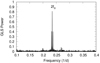 |
Fig. 1. Periodogram obtained with the V-band photometry. 2f0 = 2/Po, where |

In order to improve the accuracy of the orbital period, we selected the photometric data points with phases close to the primary minimum (0.98 ≤ Φo ≤ 1.02) and performed an analysis of observed (O) minus calculated (C) eclipse times following Sterken (2005). In this analysis, the O–C deviations can be represented as a function of the number of cycles with a straight line whose zero point and slope are the corrections needed for the (linear) ephemeris zero point and period, respectively. We included 48 instances of primary minima that were studied by Kreiner (2004) and listed in the O–C Gateway6. Additionally, we included 209 new instances of minima measured from the data listed in Table 1, excluding satellite data because of the different time system. The dataset of minima covers about 5000 cycles (i.e., 117 years of observations). Since some minimum times are published without errors, we used a simple least square fit for our analysis. Our result, displayed in Fig. 2, shows that the fit can be performed with a straight line, indicating a constant period. The new ephemeris is given by:
 (2)
(2)
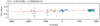 |
Fig. 2. Observed (O) minus calculated (C) epochs for primary minima versus cycle number for 117 years of observations, according to the ephemeris given by Eq. (1). Black and red dots indicate photographic and visual data, respectively. Blue, green, and magenta dots show Charge-Coupled Device (CCD) or photoelectric V-, Ic-, and g-band data, respectively. The data points with the same X and Y coordinates are displayed with a small X offset for better visualization. See Sect. 3.1. |
3.2. Search for additional photometric periods
We disentangled the light curve by removing the orbital frequency and found a long period in the residuals of the Ic-KWS band photometry: 268.7 ± 1.6 d with full amplitude 0.1096 ± 0.0066 mag. The following ephemeris was found for the minimum of the long cycle:
 (3)
(3)
No periodicity was found in the residuals of the other datasets. The periodogram showing the peak at the long-cycle frequency is shown in Fig. 3. The residual light curve phased with the long cycle is shown in Fig. 4. The peak of the Ic-band periodogram is significant and cannot be explained in terms of the data sampling.
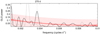 |
Fig. 3. Generalized Lomb-Scargle periodogram obtained with Ic-band data after the subtraction of the orbital period. The light gray curve shows the spectral window for the data. The best second-order polynomial fit is also shown. The 95% confidence and prediction bands are shown by dashed and dashed-light areas, respectively. |
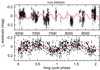 |
Fig. 4. Upper: Ic-KWS light curve after removing the orbital period. Lower: same but phased with the long period of 269 days. The best sinus fit is also shown. |
3.3. Flickering in the light curve
We observe flickering in the light curve, which was better represented in the INTEGRAL database (Fig. 5). This phenomenon consists of drops in the brightness of the light curve with regards to the mean level for a given orbital phase. This was previously reported in earlier works by Polushina (2002) as model deviations in several bands up to 0.1 mag with less time-resolved datasets. Larger variations of up to 0.2 mag over nine nights between 1972 and 1973 were recorded by Kumsiashvili & Chargeishvili (2009) but interpreted in terms of an instrumental effect. The drops in brightness observed in INTEGRAL data cannot be due to measurement errors: Individual data point errors are much smaller than the observed deviations, and the expected instrumental error for each data point for the given system magnitude is less than 0.02 mag (Mas-Hesse et al. 2003).
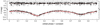 |
Fig. 5. Integral V-band data phased with the ephemeris given by Eq. (2), along with a locally weighted scatterplot smoothing curve. Residuals are shown in the upper part with data point error bars. The orbital phase has been displaced for better visualization. |
A Levenberg Marquardt nonlinear curve fit was performed with two Gaussians characterized by free parameter position, full width at half maximum, and area. The fit converged after 19 iterations with an χ2 tolerance value of 10−9 and an R-squared value of 0.977. The best fit reveals two different distributions separated by 0.062 ± 0.014 mag and whose heights are in the ratio 4.1 ± 0.6 (Fig. 6). The lower distribution is 2.4 ± 0.3 times broader than the tallest distribution. The areas of the distributions are A1 = 11.5 ± 1.0 and A2 = 6.8 ± 1.5 mag × counts. The magnitudes in the half of the smaller distribution corresponding to larger residuals (fainter magnitudes) can be identified as fading events. The corresponding ratio of areas η = 0.5A2/A1 is the relative fraction of magnitudes that can be classified as magnitude drops. We find that 29.6% of the observations correspond to fading events in this dataset. In addition, we find that the drops occur randomly; no periodicity was found in the residuals of the INTEGRAL data. The drops also appear in ASAS-SN V and g-band data (Fig. 7). The events do not have a clear dependence on the orbital phase; they appear at all phases but seem to be more abundant in quadratures. The larger drops amount to 0.3 mag in the V-band (i.e., a fall of roughly 30% of the total flux).
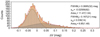 |
Fig. 6. Histogram of residuals shown in Fig. 5 modeled by the sum of two Gaussians. A non-linear fit using the Levenberg Marquardt iteration algorithm results in two distributions (black lines) and their sum (red line). The adjusted parameter’s full width at half maximum, center, area, and their errors are given for the two Gaussians. |
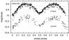 |
Fig. 7. ASAS-SN V- and g-band magnitudes phased with the ephemeris given by Eq. (2). The drops in brightness seen in INTEGRAL data are also present. Phase zero corresponds to the primary (deeper) eclipse. |
In order to investigate the time scale on which these fading events occur, we performed a correlation analysis, measuring the temporal distance between adjacent data points and the corresponding difference of magnitude. We find that jumps in magnitude on the order of 0.1 mag already occur on a time scale of minutes, and conclude that the time resolution of the data is not enough to resolve these events (Fig. 8).
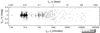 |
Fig. 8. Temporal distance between adjacent data points of all INTEGRAL V-band data plotted against the corresponding difference in magnitude. We find that flickering occurs on time scales of minutes. Data point errors are ≈0.01 mag. |
3.4. Infrared colors and W1 orbital variability
We analyzed the W1 variability and compared the infrared colors with those of double periodic variables (DPVs) and Be stars. The DPVs are close binaries that mostly consist of a B-type hotter star surrounded by an accretion disk fed by Roche-lobe overflow and mass transfer from a cooler giant companion (Mennickent 2017). Be stars are rapidly rotating B-type stars surrounded by a circumstellar disk. Both types of objects usually show color excess that is mostly attributed to circumstellar reddening; therefore, they are used here to check presence of circumstellar matter. No correction for interstellar reddening was performed. However, at these wavelengths, the effect of interstellar reddening is negligible. In addition, we included as a reference the average colors for 136 main sequence stars in the range of spectral types from B1 V to K3 V from the HIPPARCOS catalog (Perryman 1997). Further details regarding the data selection of DPVs, Be stars, and HIPPARCOS stars are available in Mennickent et al. (2016). Our results are shown in Fig. 9.
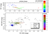 |
Fig. 9. Upper: W1 magnitude versus orbital phase according to the ephemeris given by Eq. (2). Colors represent time intervals. Lower: color-color diagram for non-variable HIPPARCOS stars of spectral type B1 V – K3 V, Be stars, and DPVs according to Mennickent et al. (2016). The UU Cas data is added with colors along with numbers (in some cases) showing the orbital phases. Phase zero corresponds to the primary (deeper) eclipse. |
We find that the light W1 magnitude follows the orbital period. Our time resolution and cadence allows for neither the resolution of the whole orbital cycle, nor the possible long cycle. Part of the variability occurs on time scales that are longer than the orbital one; this can be seen in the data acquired at the end of the time series, which deviate to brighter magnitudes compared with the rest of the data from similar orbital phases. In addition, the system appears in the W1 − W2 versus W2 − W3 diagram in an area populated by systems with circumstellar envelopes, far from the place where the HIPPARCOS non-variable stars are located. This finding strongly suggests that circumstellar matter is also present in UU Cas. Additionally, during the orbital cycle, the system transits mostly along the W1 − W2 axis, tracing a horizontal path in the color-color diagram.
The same tendency is found when comparing the published 2MASS J − H (0.194) versus H − K (0.274) colors of UU Cas (Skrutskie 2006) with those of synthetic models for dwarfs and giants, along with observed colors of Be stars and DPVs (Fig. 10). The UU Cas system is located in a similar area with regards to the DPVs, suggesting the existence of circumstellar matter and, potentially, an accretion disk.
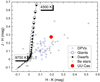 |
Fig. 10. Colors for Galactic DPVs (Mennickent et al. 2016), Be stars (Howells et al. 2001), and synthetic stellar atmosphere models with log g = 4.0 (squares with lines) and log g = 3.0 (open circles with lines) from Bessell et al. (1998). The effective temperature of two selected synthetic models have been labeled along with the position of UU Cas. |
4. Light curve model
In this section we model the orbital light curves with a theoretical code that solves the inverse problem considering a semidetached system consisting of a less massive and cooler “donor” star and a more massive and hotter “gainer” star surrounded by an accretion disk that is both optically and geometrically thick (Djurašević 1992a,b, 1996). The model includes hot and bright spots in the disk, following evidence found in previous observations of algols (Richards 2004). These active regions influence the shape of the light curve during the ingress and egress of the eclipses. The temperature of the disk matches the temperature of the gainer on its inner edge and decreases with a radial profile described by an exponent aT. The model has been described in several papers, such as Mennickent & Djurašević (2013), Mennickent et al. (2015), Mennickent (2019), where more details can be found.
We fixed the donor temperature and mass ratio to Tc = 22 700 K and q = 0.52, in line with results from spectroscopic studies by Kononov et al. (2019) and Gorda (2017) as well as our own work based on the disentangling of spectra (work in preparation). We also assumed synchronous rotation for the donor, as expected for a close binary that rapidly synchronizes stellar spins with the orbit due to tidal forces. On the other hand, the gainer might have been spun-up to a high rotation due to nearly tangentially infalling material (Packet 1981), hence we assumed a critical rotation for it. For Ic data, we modeled the residuals after subtracting the long cycle.
The parameters of the best fits are shown in Table 2. Multi-color KWV-UBV and P02-UBVR data were fit independently and parameters were averaged. Examples of fits to the KWS-Ic and INTEGRAL V-band light curves are shown in Fig. 11. We obtain a good match between observed and calculated magnitudes in all studied cases, along with consistency for the stellar and orbital parameters. The disk parameters show some variations, notably the bright spot position, the spot temperature, and the disk’s vertical thickness and radius. Our model indicates a system seen at an angle of 74° and a stellar separation of 52 R⊙. The stellar temperatures are 22 700 K and 30 200 K. The stellar masses are 9 and 17.4 M⊙, and surface gravities are log g = 2.94 and 3.98. The stellar radii are 16.9 and 7.0 R⊙. The stellar temperatures indicate spectral types of B 2 and B 0 for the donor and gainer stars, respectively (Harmanec 1988).
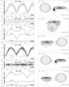 |
Fig. 11. Observed (LCO) and synthetic (LCC) light curves of UU Cas obtained by analyzing: KWS-Ic data and INTEGRAL V-band photometric observations; final O–C residuals between the observed and optimum synthetic light curves; fluxes of the donor, gainer, and accretion disk, normalized to the donor flux at phase 0.25; and the views of the optimal model at orbital phases 0.20, 0.48, and 0.80 (Ic-KWS) and 0.20 and 0.80 (INTEGRAL), obtained with parameters estimated by the light curve analysis. |
Results of the analysis of UU Cas orbital light curves.
The disk radius is relatively stable around a value of 21 R⊙, reaching its minimum value at 18 R⊙ (INTEGRAL-V data) and its maximum value at 22 R⊙ (P02 data). It has a temperature of 16 000 K at its outer edge. The inner disk’s thickness has an average value of 9 R⊙, and the outer vertical thickness has an average value of 6.5 R⊙ and a maximum of 9.4 R⊙ (KWS-Ic data). The hot spot is 36% (P02 data) to 70% (KWS-Ic data) hotter than the disk and is located consistently 42° from the line joining the stellar centers in the direction opposite to the orbital motion (i.e., it is located roughly at the expected region where the gas stream impacts the disk). The bright spot is 24% (P02 data) to 50% (KWS-Ic data) hotter than the disk and changes its location considerably, located between 82° (KW data) and 141° (KWS-g data) from the line joining the stellar centers in the direction of the orbital motion. At quadratures, the flux ratio between the donor and the disk is ≈2 in the Ic-band, while in the V-band this ratio is ≈3. The gainer is almost completely hidden by the disk at all orbital phases, contributing less than 10% of the total flux in both bands.
5. Discussion
Our results confirm the picture summarized by Gorda (2017) and Kononov et al. (2019) of a semidetached binary where the less massive star feeds an accretion disk located around the more massive and partly hidden star. Our light curve models, which are based on 11 different datasets obtained at different epochs and with different photometric bands, indicate consistent results for the overall system configuration, especially the orbital and stellar parameters, consolidating the overall view of a massive interacting binary of early B-type components.
Our light curve models indicate a system of B0 IV + B2 III stars with a relatively large total mass of about 26 M⊙. Our stellar masses of 17.4 and 9 M⊙ are relatively close to those reported by Gorda (2017), namely 17.7 and 9.5 M⊙. The mass, radius, and temperature of the more massive component fit the relationships for B-type dwarfs reported by Harmanec (1988) well. However, the less massive component is much larger than expected for its temperature, which indicates an evolved star, consistent with its lower surface gravity. In addition, we find an accretion disk around the more massive star and derive, for the first time, their properties. The average disk radius of 21 R⊙ means Rd/a ≈ 0.40, that is to say, the disk’s outer border is just below the tidal radius for the given mass ratio (Paczyński 1977; Warner 1995a). The disk radius shows small changes during the observing epochs, while the disk is characterized by two hot and active photometrically variable regions. The changes in these regions (position, extension, temperature) might indicate changes in the mass transfer rate that modulate the mass flows and disk properties. The infrared excess obtained in our photometric study confirms the existence of circumstellar matter, while the enigmatic obscuration events mostly visible in INTEGRAL V-data might be related to inhomogeneities present in the flow of mass loss. The existence of these fading events suggests a mass flow structure more complex than that provided by our simple model of disk plus two spots. In the future, new, higher-accuracy data could add new constraints and improve the understanding of the system.
The long period observed in the Ic-band and the light curve morphology suggests that UU Cas might be a DPV (Mennickent et al. 2003; Mennickent 2017), a subtype of algols that shows β-Lyrae-type light curves that have an accretion disk surrounding a B-type gainer. At red passbands, DPVs show long cycles of larger amplitudes (Michalska et al. 2010). This might indicate that the long cycle arises from a light source emitting mostly at wavelengths that are redder than the other sources in the system. This could explain why the long cycle is detected (with a small amplitude) only in the Ic-band in UU Cas. All DPVs (except β Lyrae) show a constant orbital period despite evidence of active mass exchange and occasional mass outflows. All these credentials are similar to those of UU Cas. In addition, the ratio between the long-cycle length and the orbital period is 31.7 for UU Cas, relatively close to the average ∼33 for DPVs. Since the long period is observed only in one dataset, we would need confirmation with additional data before claiming that UU Cas is a DPV. If confirmed, UU Cas would be the most massive DPV known to date; they typically only have total masses around 10 M⊙.
The reported evidence for an Hα P-Cygni-like profile led Gorda (2017) to conclude that a stellar wind emerges from the system. This might indicate that the system is losing mass. However, the constancy of the orbital period over one century suggests that this mass loss is mild, that is to say the angular momentum of the system remains almost unaltered, as does the orbital period. This is consistent with a binary in a relatively stable and mild mass-transfer stage.
The error in the orbital period ϵ = 0 000008, given by Eq. (2), might be interpreted as a possible drift of the orbital period between Po − ϵ and Po + ϵ in Δt = 117 years. This implies a possible change in the orbital period of less than roughly 2ϵP/Δt = 1.37 × 10⁻⁷ d yr−1. For conservative mass transfer, this imposes an upper limit for the mass transfer rate. The expected period change in the conservative case is (Huang 1963):
 (4)
(4)
Using the aforementioned numbers and the derived stellar masses, we determine  < 1.0 × 10⁻⁷ M⊙ yr−1.
6. Conclusions
Based on the analysis of multiwavelength light curves and published spectroscopic results, we have arrived at the following conclusions:
-
We find that an improved orbital period of
 seems to have remained stable over the last century. This suggests that the rate of system mass loss or mass exchange between the stars is small.
 -
We find a long cycle of length T ∼ 270 d in the Ic-band data.
-
We find a system seen at an angle of 74° with a stellar separation of 52 R⊙. The stellar temperatures are 22 700 K and 30 200 K, masses are 9 and 17.4 M⊙, radii are 16.9 and 7.0 R⊙, and surface gravities are log g = 2.94 and 3.98.
-
The system follows a horizontal path in the W1 − W2 versus W2 − W3 diagram and is located in the region of systems containing circumstellar matter like DPVs and Be stars. The location in the J − H versus H − K diagram also suggests infrared excess due to circumstellar matter.
-
We find an accretion disk around the hotter star, with a radius of 21 R⊙. Two active regions are found, one located roughly in the expected position (where the stream impacts the disk) and the other on the opposite side of the disk. Changes are observed in the disk and spot parameters at different datasets; this might indicate a variable mass transfer rate.
-
We find that the light curves show enigmatic obscuration events consisting of rapid drops in brightness of up to ΔV = 0.3 mag. These events might be related to inhomogeneities present in the flow of mass loss, but more studies are needed to clarify their nature.
Acknowledgments
We thank the anonymous referee that helped to improve the first version of this manuscript. R. E. M., J. G. and M. C. acknowledge support by BASAL Centro de Astrofísica y Tecnologías Afines (CATA) PFB-06/2007 and FONDECYT 1190621. JG acknowledges ANID project 21202285. G. D., I. V., J. P. and M. I. J. acknowledge the financial support of the Ministry of Education, Science and Technological Development of the Republic of Serbia through the contract No 451-03-68/2020/14/20002. M. C. and P. H. acknowledge support by Astronomical Institute of the Czech Academy of Sciences through the project RVO 67985815. D. K. thanks GA 17-00871S of the Czech Science Foundation. H.M. acknowledges to the Bulgarian National Science Fund under contract DN 18/13-12.12.2017. This research has made use of: (1) the SIMBAD database, operated at CDS, Strasbourg, France (Wenger et al. 2000), (2) data products from the Wide-field Infrared Survey Explorer, which is a joint project of the University of California, Los Angeles, and the Jet Propulsion Laboratory/California Institute of Technology, funded by the National Aeronautics and Space Administration, (3) the NASA/ IPAC Infrared Science Archive, which is operated by the Jet Propulsion Laboratory, California Institute of Technology, under contract with the National Aeronautics and Space Administration, (4) data products from the Two Micron All Sky Survey, which is a joint project of the University of Massachusetts and the Infrared Processing and Analysis Center/California Institute of Technology, funded by the National Aeronautics and Space Administration and the National Science Foundation and (5) data from the OMC Archive at CAB (INTA-CSIC), pre-processed by ISDC.
References
- Bailer-Jones, C. A. L., Rybizki, J., Fouesneau, M., et al. 2018, AJ, 156, 58 [NASA ADS] [CrossRef] [Google Scholar]
- Bessell, M. S., Castelli, F., & Plez, B. 1998, A&A, 333, 231 [NASA ADS] [Google Scholar]
- de Mink, S. E., Sana, H., Langer, N., et al. 2014, ApJ, 782, 7 [NASA ADS] [CrossRef] [Google Scholar]
- Djurašević, G. 1992a, Ap&SS, 196, 267 [NASA ADS] [CrossRef] [Google Scholar]
- Djurašević, G. 1992b, Ap&SS, 197, 17 [NASA ADS] [CrossRef] [Google Scholar]
- Djurašević, G. 1996, Ap&SS, 240, 317 [NASA ADS] [CrossRef] [Google Scholar]
- Djurašević, G. R., Vince, I., & Atanacković, O. 2010, in Binaries - Key to Comprehension of the Universe. Proceedings of a conference held June 8-12, 2009 in Brno, Czech Republic, eds. A. Prša, & M. Zejda (San Francisco: Astronomical Society of the Pacific), 301 [Google Scholar]
- Domingo, A., Gutiérrez-Sánchez, R., Rísquez, D., et al. 2010, Astrophys. Space Sci. Proc., 14, 493 [NASA ADS] [CrossRef] [Google Scholar]
- Gorda, S. Y. 2017, Astrophys. Bull., 72, 321 [CrossRef] [Google Scholar]
- Harmanec, P. 1988, BAICz, 39, 329 [Google Scholar]
- Howells, L., Steele, I. A., Porter, J. M., & Etherton, J. 2001, A&A, 369, 99 [NASA ADS] [CrossRef] [EDP Sciences] [Google Scholar]
- Huang, S.-S. 1963, ApJ, 138, 471 [NASA ADS] [CrossRef] [Google Scholar]
- Kononov, D. A., Gorda, S. Y., & Parfenov, S. Y. 2019, ApJ, 883, 186 [CrossRef] [Google Scholar]
- Kreiner, J. M. 2004, Acta Astron., 54, 207 [NASA ADS] [Google Scholar]
- Kruckow, M. U., Tauris, T. M., Langer, N., et al. 2018, MNRAS, 481, 1908 [NASA ADS] [CrossRef] [Google Scholar]
- Kumsiashvili, M. I., & Chargeishvili, K. B. 2009, ArXiv e-prints [arXiv:0907.1047] [Google Scholar]
- Lomb, N. R. 1976, Ap&SS, 39, 447 [Google Scholar]
- Markov, H., Vince, I., Markova, N., et al. 2010, Publications de l’Observatoire Astronomique de Beograd, 90, 159 [Google Scholar]
- Markov, H., Markova, N., Vince, I., et al. 2011, Bulgarian. Astron. J., 15, 87 [Google Scholar]
- Maehara, H. 2014, JAXA Res. Dev. Rep., 13, 119 [Google Scholar]
- Mas-Hesse, J. M., Giménez, A., Culhane, J. L., et al. 2003, A&A, 411, L261 [NASA ADS] [CrossRef] [EDP Sciences] [Google Scholar]
- Mennickent, R. E. 2017, Serb. Astron. J., 194, 1 [NASA ADS] [CrossRef] [Google Scholar]
- Mennickent, R. E., & Djurašević, G. 2013, MNRAS, 432, 799 [NASA ADS] [CrossRef] [Google Scholar]
- Mennickent, R. E., Pietrzyński, G., Diaz, M., et al. 2003, A&A, 399, L47 [NASA ADS] [CrossRef] [EDP Sciences] [Google Scholar]
- Mennickent, R. E., Kołaczkowski, Z., Djurašević, G., et al. 2012, MNRAS, 427, 607 [NASA ADS] [CrossRef] [Google Scholar]
- Mennickent, R. E., Djurašević, G., Cabezas, M., et al. 2015, MNRAS, 448, 1137 [NASA ADS] [CrossRef] [Google Scholar]
- Mennickent, R. E., Otero, S., & Kołaczkowski, Z. 2016, MNRAS, 455, 1728 [NASA ADS] [CrossRef] [Google Scholar]
- Mennickent, R. E., et al. 2019, MNRAS, 487, 4169 [CrossRef] [Google Scholar]
- Michalska, G., Mennickent, R. E., Kołaczkowski, Z., et al. 2010, in Binaries - Key to Comprehension of the Universe. Proceedings of a conference held June 8-12, 2009 in Brno, Czech Republic, eds. A. Prša, & M. Zejda (San Francisco: Astronomical Society of the Pacific), 357 [Google Scholar]
- Packet, W. 1981, A&A, 102, 17 [NASA ADS] [Google Scholar]
- Paczyński, B. 1977, ApJ, 216, 822 [NASA ADS] [CrossRef] [Google Scholar]
- Parenago, P., & Kukarkin, B. 1940, Perem Zvezdy, 5, 287 [Google Scholar]
- Perryman, M. A. C., et al. 1997, A&A, 323, L49 [Google Scholar]
- Petrovic, J., Langer, N., Yoon, S.-C., et al. 2005, A&A, 435, 247 [NASA ADS] [CrossRef] [EDP Sciences] [Google Scholar]
- Podsiadlowski, P., Joss, P. C., & Hsu, J. J. L. 1992, ApJ, 391, 246 [NASA ADS] [CrossRef] [Google Scholar]
- Polushina, T. S. 2002, Astron. Rep., 46, 900 [CrossRef] [Google Scholar]
- Polushina, T. S. 2004, Astron. Astrophys. Trans., 23, 213 [NASA ADS] [CrossRef] [Google Scholar]
- Richards, M. T. 2004, AN, 325, 229 [Google Scholar]
- Samus, N. N., Kazarovets, E. V., Durlevich, O. V., et al. 2017, Astron. Rep., 61, 80 [NASA ADS] [CrossRef] [Google Scholar]
- Sanford, R. F. 1934, ApJ, 79, 84 [CrossRef] [Google Scholar]
- Scargle, J. D. 1982, ApJ, 263, 835 [Google Scholar]
- Skrutskie, M. F., et al. 2006, AJ, 131, 1163 [NASA ADS] [CrossRef] [Google Scholar]
- Sterken, C. 2005, ASPC, 335, 3 [Google Scholar]
- Verbunt, F. 1993, ARA&A, 31, 93 [NASA ADS] [CrossRef] [Google Scholar]
- Warner, B. 1995a, Cambridge Astrophys. Ser., 28 [Google Scholar]
- Wenger, M., Ochsenbein, F., Egret, D., et al. 2000, A&AS, 143, 9 [NASA ADS] [CrossRef] [EDP Sciences] [Google Scholar]
- Wright, E. L., Eisenhardt, P. R. M., Mainzer, A. K., et al. 2010, AJ, 140, 1868 [Google Scholar]
- Zapartas, E., de Mink, S. E., Justham, S., et al. 2020, A&A, submitted, [arXiv:2002.07230] [Google Scholar]
- Zechmeister, M., & Kürster, M. 2009, A&A, 496, 577 [NASA ADS] [CrossRef] [EDP Sciences] [Google Scholar]
All Tables
Photometric time series analyzed in this paper. KW stands for Kumsiashvili & Chargeishvili (2009), KWS for Kamogata Kiso Kyoto Wide-field Survey, and P02 for Polushina (2002).
All Figures
|
Fig. 1. Periodogram obtained with the V-band photometry. 2f0 = 2/Po, where |
| In the text | |
|
Fig. 2. Observed (O) minus calculated (C) epochs for primary minima versus cycle number for 117 years of observations, according to the ephemeris given by Eq. (1). Black and red dots indicate photographic and visual data, respectively. Blue, green, and magenta dots show Charge-Coupled Device (CCD) or photoelectric V-, Ic-, and g-band data, respectively. The data points with the same X and Y coordinates are displayed with a small X offset for better visualization. See Sect. 3.1. |
| In the text | |
|
Fig. 3. Generalized Lomb-Scargle periodogram obtained with Ic-band data after the subtraction of the orbital period. The light gray curve shows the spectral window for the data. The best second-order polynomial fit is also shown. The 95% confidence and prediction bands are shown by dashed and dashed-light areas, respectively. |
| In the text | |
|
Fig. 4. Upper: Ic-KWS light curve after removing the orbital period. Lower: same but phased with the long period of 269 days. The best sinus fit is also shown. |
| In the text | |
|
Fig. 5. Integral V-band data phased with the ephemeris given by Eq. (2), along with a locally weighted scatterplot smoothing curve. Residuals are shown in the upper part with data point error bars. The orbital phase has been displaced for better visualization. |
| In the text | |
|
Fig. 6. Histogram of residuals shown in Fig. 5 modeled by the sum of two Gaussians. A non-linear fit using the Levenberg Marquardt iteration algorithm results in two distributions (black lines) and their sum (red line). The adjusted parameter’s full width at half maximum, center, area, and their errors are given for the two Gaussians. |
| In the text | |
|
Fig. 7. ASAS-SN V- and g-band magnitudes phased with the ephemeris given by Eq. (2). The drops in brightness seen in INTEGRAL data are also present. Phase zero corresponds to the primary (deeper) eclipse. |
| In the text | |
|
Fig. 8. Temporal distance between adjacent data points of all INTEGRAL V-band data plotted against the corresponding difference in magnitude. We find that flickering occurs on time scales of minutes. Data point errors are ≈0.01 mag. |
| In the text | |
|
Fig. 9. Upper: W1 magnitude versus orbital phase according to the ephemeris given by Eq. (2). Colors represent time intervals. Lower: color-color diagram for non-variable HIPPARCOS stars of spectral type B1 V – K3 V, Be stars, and DPVs according to Mennickent et al. (2016). The UU Cas data is added with colors along with numbers (in some cases) showing the orbital phases. Phase zero corresponds to the primary (deeper) eclipse. |
| In the text | |
|
Fig. 10. Colors for Galactic DPVs (Mennickent et al. 2016), Be stars (Howells et al. 2001), and synthetic stellar atmosphere models with log g = 4.0 (squares with lines) and log g = 3.0 (open circles with lines) from Bessell et al. (1998). The effective temperature of two selected synthetic models have been labeled along with the position of UU Cas. |
| In the text | |
|
Fig. 11. Observed (LCO) and synthetic (LCC) light curves of UU Cas obtained by analyzing: KWS-Ic data and INTEGRAL V-band photometric observations; final O–C residuals between the observed and optimum synthetic light curves; fluxes of the donor, gainer, and accretion disk, normalized to the donor flux at phase 0.25; and the views of the optimal model at orbital phases 0.20, 0.48, and 0.80 (Ic-KWS) and 0.20 and 0.80 (INTEGRAL), obtained with parameters estimated by the light curve analysis. |
| In the text | |
Current usage metrics show cumulative count of Article Views (full-text article views including HTML views, PDF and ePub downloads, according to the available data) and Abstracts Views on Vision4Press platform.
Data correspond to usage on the plateform after 2015. The current usage metrics is available 48-96 hours after online publication and is updated daily on week days.
Initial download of the metrics may take a while.