| Issue |
A&A
Volume 642, October 2020
|
|
|---|---|---|
| Article Number | A22 | |
| Number of page(s) | 16 | |
| Section | Stellar atmospheres | |
| DOI | https://doi.org/10.1051/0004-6361/202038787 | |
| Published online | 30 September 2020 | |
The CARMENES search for exoplanets around M dwarfs
A deep learning approach to determine fundamental parameters of target stars
1
Hamburger Sternwarte,
Gojenbergsweg 112,
21029
Hamburg,
Germany
e-mail: This email address is being protected from spambots. You need JavaScript enabled to view it.
2
Homer L. Dodge Department of Physics and Astronomy, University of Oklahoma,
440 West Brooks Street,
Norman,
OK
73019,
USA
3
Departamento de Construcción e Ingeniería de Fabricación, Universidad de Oviedo, c/ Pedro Puig Adam, Sede Departamental Oeste,
Módulo 7, 1 a planta,
33203
Gijón,
Spain
4
Departamento de Ingeniería de Organización, Administración de Empresas y Estadística, Universidad Politécnica de Madrid,
c/ José Gutiérrez Abascal 2,
28006
Madrid,
Spain
5
Centro de Astrobiología (CSIC-INTA), ESAC,
Camino bajo del castillo s/n,
28692
Villanueva de la Cañada,
Madrid,
Spain
6
Departamento de Ingeniería Mecánica. Universidad de la Rioja. San José de Calazanz 31,
26004
Logroño,
La Rioja,
Spain
7
Institut de Ciències de l’Espai (CSIC-IEEC),
Campus UAB, c/ de Can Magrans s/n,
08193
Bellaterra,
Barcelona,
Spain
8
Institut d’Estudis Espacials de Catalunya (IEEC),
08034
Barcelona,
Spain
9
Institut für Astrophysik, Georg-August-Universität,
Friedrich-Hund-Platz 1,
37077
Göttingen,
Germany
10
Landessternwarte, Zentrum für Astronomie der Universtät Heidelberg,
Königstuhl 12,
69117
Heidelberg,
Germany
11
Instituto de Astrofísica de Andalucía (IAA-CSIC),
Glorieta de la Astronomía s/n,
18008
Granada,
Spain
12
Centro Astronómico Hispano-Alemán (CSIC-MPG), Observatorio Astronómico de Calar Alto,
Sierra de los Filabres,
04550
Gérgal,
Almería,
Spain
13
Instituto de Astrofísica de Canarias,
c/ Vía Láctea s/n,
38205
La Laguna,
Tenerife,
Spain
14
Departamento de Astrofísica, Universidad de La Laguna,
38206
La Laguna,
Tenerife,
Spain
15
Thüringer Landessternwarte Tautenburg,
Sternwarte 5,
07778
Tautenburg,
Germany
16
Max-Planck-Institut für Astronomie,
Königstuhl 17,
69117
Heidelberg,
Germany
17
Departamento de Física de la Tierra y Astrofísica and IPARCOS-UCM (Instituto de Física de Partículas y del Cosmos de la UCM), Facultad de Ciencias Físicas, Universidad Complutense de Madrid,
28040
Madrid,
Spain
18
Departamento de Inteligencia Artificial, UNED, Juan del Rosal, 16,
Madrid
28040,
Spain
19
Instituto de Astrofísica e Ciências do Espaço, Universidade do Porto, CAUP, Rua das Estrelas,
4150-762
Porto,
Portugal
Received:
29
June
2020
Accepted:
27
July
2020
Abstract
Existing and upcoming instrumentation is collecting large amounts of astrophysical data, which require efficient and fast analysis techniques. We present a deep neural network architecture to analyze high-resolution stellar spectra and predict stellar parameters such as effective temperature, surface gravity, metallicity, and rotational velocity. With this study, we firstly demonstrate the capability of deep neural networks to precisely recover stellar parameters from a synthetic training set. Secondly, we analyze the application of this method to observed spectra and the impact of the synthetic gap (i.e., the difference between observed and synthetic spectra) on the estimation of stellar parameters, their errors, and their precision. Our convolutional network is trained on synthetic PHOENIX-ACES spectra in different optical and near-infrared wavelength regions. For each of the four stellar parameters, Teff, log g, [M/H], and v sin i, we constructed a neural network model to estimate each parameter independently. We then applied this method to 50 M dwarfs with high-resolution spectra taken with CARMENES (Calar Alto high-Resolution search for M dwarfs with Exo-earths with Near-infrared and optical Échelle Spectrographs), which operates in the visible (520–960 nm) and near-infrared wavelength range (960–1710 nm) simultaneously. Our results are compared with literature values for these stars. They show mostly good agreement within the errors, but also exhibit large deviations in some cases, especially for [M/H], pointing out the importance of a better understanding of the synthetic gap.
Key words: methods: data analysis / techniques: spectroscopic / stars: fundamental parameters / stars: late-type / stars: low-mass
© ESO 2020
1 Introduction
The determination of stellar parameters in M dwarfs has always been challenging. M dwarfs are smaller, cooler, and fainter than Sun-like stars. Due to their faintness, higher stellar activity with sometimes strong magnetic fields, stronger line blends, and the lack of true continuum, well-established photometric and spectroscopic methods are brought to their limits. In the literature there are several methods to estimate M-dwarf parameters such as effective temperature Teff, surface gravity log g, and metallicity. In particular, the measurement of spectral line pseudo-equivalent widths (pEWs) is a widely used method for metallicity determination. Neves et al. (2013, 2014) measured pEWs for the HARPS guaranteed time observations of M dwarfs and calibrated them with photometric relations from Neves et al. (2012) for metallicity and from Casagrande et al. (2008) for effective temperature. Metallicity relations based on equivalent widths were derived by Newton et al. (2014) using low-resolution spectra (R ~ 2000) in the J, H, and K bands. They calibrated their method with binary systems with an F-, G-, or K-type primary and an M-dwarf secondary. Pseudo-EWs in the K- and H-band and H2O indices were measured by Khata et al. (2020) to determine metallicities and effective temperatures as well as radii, luminosities, spectral types, and absolute magnitudes for 53 M dwarfs. Combining pEWs with empirical calibrations and spectral synthesis, Veyette et al. (2017) derived Teff and Ti and Fe abundances for 29 M dwarfs with high-resolution Y -band spectra.
A method considered to be very precise is the calibration with M dwarfs that have an F, G, or K binary companion with known metallicity. Many of the above mentioned relations were calibrated using FGK+M binary systems (e.g., Newton et al. 2014). Mann et al. (2013a) identified metallicity sensitive features in low-resolution visible, J-, H-, and K-band spectra of 112 late-K to mid-M dwarfs in binary systems with higher mass companions, from which they derived different metallicity calibrations.The same relations were used by Rodríguez Martínez et al. (2019) to determine metallicities from mid-resolution K-band spectra for 35 M dwarfs of the K2 mission. Other photometric calibrations using FGK+M binary systems are presented by Bonfils et al. (2005), Casagrande et al. (2008), Johnson & Apps (2009), Schlaufman & Laughlin (2010), and Neves et al. (2012), among others. Several spectroscopic calibrations can be found in Rojas-Ayala et al. (2010), Dhital et al. (2012), Terrien et al. (2012), Mann et al. (2014, 2015), and Montes et al. (2018).
Another approach to determine stellar parameters for M dwarfs is the calculation of different kinds of spectral indices. Many of these indices were calibrated using FGK+M binaries, as mentioned above. Gaidos & Mann (2014) derived Teff from K-band M-dwarf spectra by calculating spectral curvature indices. For metallicity they used relations of atomic line strength based on Mann et al. (2013a). Also working in the K band, Rojas-Ayala et al. (2012) calculated the H2O-K2 index, quantifying the absorption from H2O opacity, to determine Teff from low-resolution (R ~ 2700) M-dwarf spectra. Newton et al. (2015) measured 13 spectral indices and 26 pEWs in the near-infrared H band to estimate metallicities of the MEarth transiting planet survey and the cool Kepler objects of interest. For temperature determination they employed the H2O-K2 index from Rojas-Ayala et al. (2012) and spectral indices from Mann et al. (2013b). Molecular indices of CaH and TiO were calculated by Woolf & Wallerstein (2006) to derive a relation between those indices and metallicities for 76 late-K and M dwarfs. To test their results, they compared measurements of several M dwarfs with higher mass companions to the metallicities of the primaries and find good agreement. Johnson et al. (2012) combined several existing photometric relations to derive the stellar properties of KOI-254.
Stellar parameters can also be derived from interferometric measurements. However, only a limited number of stars is accessible for such observations, since they have to be bright and nearby. Boyajian et al. (2012) present interferometric angular diameters for 26 K and M dwarfs measured with the CHARA array and for seven K and M dwarfs from the literature. With parallaxes and bolometric fluxes they computed absolute luminosities, radii, and Teff. They also calculated empirical relations for K0 to M4 dwarfs to connect Teff, radius, and luminosity to broadband color indices and [Fe/H]. Maldonado et al. (2015) estimated Teff from pEWs calibrated with interferometric temperatures from Boyajian et al. (2012) and metallicities from pEWs calibrated with the Neves et al. (2012) relations. They constructed a mass-radius relation using interferometric radii (Boyajian et al. 2012; von Braun et al. 2014) and masses from eclipsing binaries (Hartman et al. 2015). From this they calculated surface gravities, log g. Other works that derived Teff from angular diameters include, for example, Ségransan et al. (2003), Demory et al. (2009), von Braun et al. (2014), and Newton et al. (2015). Of them, Ségransan et al. (2003) also determined log g from their measured masses and radii.
A not very commonly used method for stellar parameter determination is the principle component analysis. Paletou et al. (2015) and He & Zhao (2019) show that this method could in principle be used to derive effective temperature for K- and M-type stars and abundances for dwarfs and giants, respectively.
With the improvement of synthetic models for cool stellar atmospheres, model fits to low- or high-resolution spectra are getting more powerful. Several model sets are based on the stellar atmosphere code PHOENIX (Hauschildt 1992, 1993). The BT-Settl models (Allard et al. 2012, 2013) were used by Veyette et al. (2017) and Rajpurohit et al. (2018), who determined Teff, log g, and metallicities for M dwarfs from CARMENES high-resolution spectra (Reiners et al. 2018). Gaidos & Mann (2014) and Mann et al. (2015) also derived Teff of M dwarfs from fitting BT-Settl models, but to low-resolution visible SNIFS spectra. Kuznetsov et al. (2019) determined Teff, log g, [Fe/H], and v sin i of 153 M dwarfs by fitting mid-resolution visible spectra from X-shooter at VLT using BT-Settl models.
Zboril & Byrne (1998) (see also Zboril et al. 1998) fitted PHOENIX models (Allard & Hauschildt 1995) to derive log g and [M/H] for 11 M dwarfs with high-resolution visible spectra. To estimate Teff they used photometric indices. Bean et al. (2006) generated synthetic spectra based on the PHOENIX NextGen models (Hauschildt et al. 1999) using the stellar analysis code MOOG (Sneden 1973) to determine Teff and [M/H] for three planet-hosting M dwarfs. After several recent updates of line lists and the equation of state, the PHOENIX models were used by Passegger et al. (2018) (PHOENIX-ACES, see Husser et al. 2013), Passegger et al. (2019), and Schweitzer et al. (2019) (both using the SESAM equation of state, see Meyer 2017) to derive Teff, log g, and [Fe/H] of M dwarfs observed with CARMENES in the visible and near-infrared wavelength ranges. Birky et al. (2017) determined the same parameters for late-M and early-L dwarfs from fitting PHOENIX models to high-resolution near-infrared APOGEE spectra (R ~ 22 500). Another source for synthetic models widely used are the MARCS model atmospheres (Gustafsson et al. 2008). Önehag et al. (2012) used MARCS atmospheres together with the SME package (Valenti & Piskunov 1996; Valenti & Fischer 2005) to calculate synthetic models with specific parameters on the fly and to fit them to high-resolution J-band spectra of eight M dwarfs. Souto et al. (2017) generated synthetic spectra using the Turbospectrum code (Alvarez & Plez 1998; Plez 2012) and MARCS atmospheres and fitted them to high-resolution APOGEE spectra of two M-dwarf exoplanet hosts to determine 13 element abundances. Souto et al. (2018) employed MARCS and BT-Settl model atmospheres (Allard et al. 2013) together with Turbspectrum to find Teff, log g, and eight element abundances of the exoplanet host Ross 128 (M4.0 V). Recently, Souto et al. (2020) used the Turbospectrum code and MARCS atmospheres with updated APOGEE atomic and molecular line lists (Shetrone et al. 2015) to calculate synthetic spectra and fitted them to 21 M-dwarf high-resolution H-band spectra observed with APOGEE.
In recent years, machine learning (ML) has proved to be a powerful tool in many fields and also found its way into astrophysics and stellar parameter determination. Machine learning techniques are used in several areas of astrophysics, such as galaxy morphology prediction (Dieleman et al. 2015) and classification (Wu et al. 2018), detection of bar structures in galaxy images (Abraham et al. 2018), determining the evolutionary states of red giants from asteroseismology (Hon et al. 2017), and classifying variable stars from analysis of light curves (Mahabal et al. 2017). Early applications of neural networks to characterize stellar spectra can be found in von Hippel et al. (1994), Gulati et al. (1994), and Singh et al. (1998), for example. Bailer-Jones et al. (1997) trained an artificial neural network with synthetic spectra to determine Teff, log g, and [M/H] for over 5000 stars of spectral types B to K.
Sharma et al. (2019) compared different ML algorithms, such as artificial neural networks (ANN), random forests, and convolutional neural networks, to classify stellar spectra. They report that their convolutional neural network achieved better accuracy than the other ML algorithms, and point out the importance of a sufficiently large training set. Sarro et al. (2018) used genetic algorithms for selecting features such as equivalent widths and integrated flux ratios from BT-Settl model atmospheres. They estimated Teff, log g, and [M/H] for M dwarfs with eight different regression models and ML techniques, and compared the results to classical χ2 and independent component analysis coefficients. Whitten et al. (2019) present the Stellar Photometric Index Network Explorer (SPHINX), an artificial neural network approach to estimate Teff and [Fe/H] from J-PLUS broad- and intermediate-band optical photometry, and synthetic magnitudes. SPHINX is able to successfully estimate temperatures and metallicities for stars in the range 4500 K < Teff < 8500 K and down to [Fe/H] ~−3.
The Cannon (Ness et al. 2015) and The Cannon2 (Casey et al. 2016) were designed to derive stellar parameters from APOGEE spectra. The Cannon is a data-driven approach that is trained with observed spectra with known parameters from the APOGEE pipeline. For training they used only 542 reference stars. They show that The Cannon is able to provide accurate Teff, log g, and [Fe/H] for all 55 000 stars of APOGEE DR10, even for those with low signal-to-noise ratio (S/N) around 50. Birky et al. (2020) also used The Cannon and determined Teff, log g, [Fe/H], anddetailed abundances for 5875 M dwarfs from the APOGEE and Gaia DR2 surveys.
Fabbro et al. (2018) trained the convolutional neural network StarNet on observed APOGEE spectra as well as synthetic MARCS and ATLAS9 model atmospheres. They applied StarNet to 148 724 and 21 787 stars, respectively, with temperatures between 4000 K and 5000 K, and measured Teff, log g, and [Fe/H]. They find that StarNet is capable of deriving parameters close to those determined from the APOGEE pipeline when trained with observed spectra, although there are some larger differences for lower metallicities and higher temperatures. For StarNet trained on synthetic spectra the intrinsic error is about twice as large than for observed spectra, although the resulting parameters are very similar. Additionally, Fabbro et al. (2018) gave a detailed description on neural networks. Leung & Bovy (2019) also derived stellar parameters for the whole APOGEE dataset using the Bayesian neural network astroNN, which was trained with observed spectra from the APOGEE pipeline over the full spectral range. Additionally, they determined 19 individual element abundances from specific wavelength ranges using mini-networks.
Recently, Antoniadis-Karnavas et al. (2020) present their ML tool ODUSSEAS, which is based on measuring pEWs of more than 4000 absorption lines in the optical. They trained their neural network with a set of HARPS spectra consisting of only 45 training and 20 test spectra. ODUSSEAS can be applied to spectra with different resolutions because the tool adjusts the resolution of the HARPS spectra in the training step. Thanks to this capability, Antoniadis-Karnavas et al. (2020) successfully derived Teff and [Fe/H] for several M dwarfs observed with different instruments.
In the study presented here we follow two main interests. First of all, we are interested in providing insights into the capability of deep learning (DL, Sect. 2.1) to create models able to learn stellar parameters when different configurations (i.e., architectures, wavelength windows, combinations of stellar parameters) are considered. Despite the regularly found astrophysical applications of DL models (Li et al. 2017; Fabbro et al. 2018; Shallue & Vanderburg 2018), we want to gain better understanding of the effects that different DL architectures have in the model creation, as well as to understand the significance of different spectral windows adopted to create models. The second interest is about considering the uncertainty induced when the training process is carried out on synthetic spectra and parameter estimation is made for observed spectra, which is not the common way of using DL models. To do this we applied the DL method to a test sample of 50 M dwarfs with high-resolution and high-S/N spectra to demonstrate the applicability of ANNs, trained with synthetic PHOENIX-ACES models (Husser et al. 2013), to observed spectra.
In Sect. 2 we explain the DL procedure and our ANN architecture. Section 3 describes the PHOENIX-ACES synthetic model grid that we used for training the neural network, our strategy of spectrum preparation, the stellar sample, and the application of our neural network. The derived stellar parameters are presented in Sect. 4, together with a literature comparison and discussion. Finally, in Sect. 5 we give a short summary of this work.
2 Method
2.1 Deep learning
Artificial intelligence is a broad area of computer science that develops systems able to perform tasks that are regularly seen to require human intelligence (McCarthy & Hayes 1981; Steels 1993; González-Marcos et al. 2013). Machine learning is an artificial intelligence technique looking to develop algorithms that can be “taught” how to learn patterns from data, instead of just transforming them. The ANN stands for a family of ML methods aiming to learn from data in a way inspired by the human brain structure (Zhang et al. 1998; Anthony & Bartlett 2009; Gong & Ordieres-Meré 2016). An ANN is constructed from different layers that are composed of a collection of artificial neurons or nodes. A node is characterized as a linear function of its input signals with weights. It is activated by a nonlinear activation function that can adopt different expressions. Some of the most commonly used functions are linear, rectified linear unit (ReLU), sigmoid, or softmax.
Deep learning is a subset of ML methods that enables computational models consisting of multiple processing layers to learn representations of data with multiple levels of abstraction (LeCun et al. 2015; Schmidhuber 2015; Zheng et al. 2018). The main difference between traditional ML and DL techniques is that in ML the feature identification needs to be established by the user, whereas in DL the features are explored in an automatic way by means of different techniques, such as convolutional transformations of the input space data.
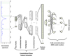 |
Fig. 1 Generic architecture for DL models in this work. |
2.2 ANN architectures
The DL techniques employed in this paper utilize two different processing units to carry out the process. Firstly, a convolutional block creates feature sets starting from a single wavelength range of the one-dimensional spectrum, in this case a synthetic model created with known stellar parameters, and it ends with a large set of created features. Next, an ANN block implements a regressive modeling approach against the stellar parameter of interest (see Fig. 1).
The ANN is built of neuron nodes organized by layers where every node is fully connected together with a feed-forward sequence, meaning that every output signal of the previous layer is connected to each node of the following layer. Regarding the layer structure of the ANN, its input layer is the set of created features from the previous convolutional block, and the output layer is the predicted stellar parameter. In between those layers, there are several hidden layers consisting of neurons. The more hidden layers the ANN contains, the “deeper” it is. This structural configuration of DL models enables the processing of data with a nonlinear approach, not only because of the convolutional nature of its preprocessing steps, but also because the activation functions in the neurons of these ANNs are commonly nonlinear, such as the ReLU (Petersen & Voigtlaender 2018).
Regarding the convolutional block, the input layer is the one-dimensional synthetic spectrum, and is followed by several convolutional layers. In these layers the weights are applied as multipliers with tunable coefficients. When considered as a matrix operation, they can be seen as a filter to the input signal (the normalized flux values of the spectrum). These filters scan across the previous layer and convolve a certain section of the input with the weights to extract features from the previous layer. Later on, the ANN learns which features are the most relevant, and it correspondingly adjusts the filter coefficients. During or just after the convolutional layers a pooling layer can be included. The function of pooling layers is to progressively reduce the spatial size of the representation to decrease the amount of free parameters and computation in the network. It can be imagined as a window sliding across the previous convolutional layer, which calculates a function value of each sub-region (e.g., its average, its maximum, etc.). By selecting the maximum value, the designer of the DL architecture extracts the strongest overall features from the convolutional layer. In this case the layer is called max pooling layer. A structural schematic is presented in Fig. 1.
2.3 Training
The DL model has a number of tunable parameters. In the following we refer to them as model parameters, in contrast to stellar parameters, which are the output of the DL model. These model parameters include number and length of filters in each convolutional layer, filter coefficients, pooling window size, and number and weights of connection nodes in the fully connected layers. At the beginning of the training phase the weights and coefficients are randomly set and get improved during the training. The training requires a reference set, which consists of a large number of observed or, in our case, synthetic spectra with known stellar parameters. Although there is not an explicit formula linking the number of training samples and the error quantifying the performance of the model, still such a relationship does exist. The higher the number of training samples, the easier to get models with acceptable mean square error (MSE) and the more accurate the final stellar parameters will be. The way to increase the number of such training dataset is to reduce the parameter’s step size in the training grid, for example by interpolation (see Sect. 3.2). A limitation on the maximum number of training samples is given by the computing feasibility according to the available resources (GP-GPU memory and data transfer throughput). Also, since the DL is able to interpolate between the synthetic grid points to some extent, minimizing the step size would not add any additional value to the derived parameters.
The reference set is divided into a training set (95%) and a validation set (5%). During the training process the whole training set is fed into the DL model, all weights and filters are applied to the input flux in each layer, and stellar parameters are predicted. The obtained output depends on the model parameters but also on the DL architecture, such as the number of convolutions, pooling layers, the number of layers of the ANN, and the chosen type of activation functions. After the whole training set is processed, the output stellar parameters are compared to the known input stellar parameters, and the training error is estimated. This error is used to modify all the DL model parameters through a backward propagation using a gradient-based algorithm and a new training cycle starts. Each of those cycles are called an “epoch.”
Additionally, after each epoch the whole validation set is sent through the DL model to determine the validation error, which is estimated to be the MSE. In this case the background idea is not to correct the error, but to have an independent estimation of the error to be measured through epochs and to avoid over-fitting of the training dataset. Over-fitting happens when the DL model describes the random variations in the dataset (e.g., tiny molecular features that appear as noise to the DL model) instead of the relations between variables (here, the stellar parameters). In this way the DL model moves from a regression into a memory tool. Obviously, this evolution negatively impacts the ability of the model to generalize to new data. With the validation set, the learned DL model is evaluated regarding its performance on unseen data. We created a regression approach able to estimate stellar parameters and not a system to identify or classify the training dataset like a memory. Keeping the validation error consistently decreasing indicates that the adjustment of weights and coefficients progresses in the right direction to improve the DL model.
The training continues until the minimum of the validation error is reached and, then, all weights and coefficients are fixed. It was commonly found after around 15 epochs. However, to be conservative, the algorithm usually ran between 35 and 50 epochs. The architecture, that is the number of layers and sequence of convolutions, was provided before the training starts and was kept fixed during the process.
2.4 Testing
The trained DL model is then applied to the test set, which in this case was a randomly generated set of 100 synthetic spectra, not related to the reference set (i.e., never seen before, neither for training nor for validation). From this set, which is preserved during all the experiments, the quality of the created models is measured through the test error. If the DL model performs well, which means that the average of the test error is lower than an adopted threshold depending on the stellar parameter under consideration, the training phase is considered complete and the DL model is applied to predict stellar parameters in observed spectra.
In our particular case, for each stellar parameter, an individual DL model was built to predict Teff, log g, [M/H], and v sin i separately, although several experiments were also conducted for predicting several parameters from the same model. The analysis of the architectures for each of these models is presented in Sect. 4.1.
3 Analysis
3.1 Observational sample
To test our DL method we used the same template spectra as in Passegger et al. (2019, in the following referred to as Pass19) and applied it to the first 50 stars listed in their Table B.1. The stellar sample that we used in this work is presented in Sect. 4 together with the results.
The spectra were observed with the CARMENES1 instrument, installed on the Zeiss 3.5 m telescope at the Calar Alto Observatory, Spain. CARMENES combines two highly stable fiber-fed spectrographs covering a spectral range from 520 to 960 nm in the visible (VIS) and from 960 to 1710 nm in the near-infrared (NIR), with spectral resolutions of R ≈ 94 600 and 80 500, respectively (Quirrenbach et al. 2018; Reiners et al. 2018). The primary goal of this instrument is to search for Earth-sized planets in the habitable zones of M dwarfs.
For a detailed description on data reduction we refer to Zechmeister et al. (2014), Caballero et al. (2016), and Pass19. As in the latter we used the high-S/N template spectrum for each star. These templates are a byproduct of the CARMENES radial velocity pipeline serval (SpEctrum Radial Velocity AnaLyser; Zechmeister et al. 2018). In the standard data flow, the code constructs a template for every target star from at least five individual spectra to derive the radial velocities of a single spectrum by least-square fitting against the template. For our sample, this results in an average S/N of around 159 for the VIS and 328 for the NIR.
Before creating the templates, the near-infrared spectra were corrected for telluric lines. We did not use the telluric correction for the visible spectra because the telluric features are negligible in the investigated ranges. The telluric correction isexplained in detail by Nagel et al. (2020). A telluric absorption spectrum was modeled for each observation using the telluric-correction tool Molecfit (Kausch et al. 2014; Smette et al. 2015) and then subtracted from the observed spectrum. The result is a telluric-free observed spectrum that can then be used to construct a template.
PHOENIX grid for DL training.
3.2 Synthetic model grid
To train the neural network, we used synthetic model spectra. The advantage of this approach is that we could generate a large enough number of model spectra and did not have to rely on a limited sample of observations with well known stellar parameters. On the other hand, although significant improvements were made in the past years (Allard et al. 2013; Husser et al. 2013), synthetic models still cannot fully model stellar atmospheres, especially in the low-temperature range. This is shown by Pass19, for example.
In this work we used the PHOENIX atmosphere code (Hauschildt 1992, 1993; Hauschildt & Baron 1999), in particular the PHOENIX-ACES models presented by Husser et al. (2013). The code generates one-dimensional model atmospheres. They can be computed in local thermodynamical equilibrium (LTE) or non-LTE radiative transfer mode for main sequence stars, brown and white dwarfs, giants, accretion disks, and expanding envelopes of novae and supernovae. As an end product, one- or three-dimensional synthetic spectra can be calculated.
Several model atmosphere grids used the PHOENIX code as a basis. This includes the NextGen (Hauschildt et al. 1999), AMES (Allard et al. 2001), BT-Settl (Allard et al. 2011), and PHOENIX-ACES models (Husser et al. 2013). The latter ones were especially designed for cool dwarfs (Teff ≥ 2300 K), as they used a new equation of state that accounts for molecule formation in low-temperature stellar atmospheres. The grid that we used in this work is based on the PHOENIX-ACES model grid.
The existing grid (step size of 100 K for Teff, and 0.5 dex for log g and [M/H]) of stellar spectra was linearly interpolated between the grid points using pyterpol (Nemravová et al. 2016). As shown in Pass19, linear interpolation between these grid points produces synthetic spectra that are numerically equivalent to results of simulated spectra. The final grid characteristics used for analyzing the DL modeling capabilities can be seen in Table 1. However, to train models to be applied to the observed spectra, additional restrictions must be considered because the whole grid can provide extra combinations of parameters that are not realistic for M stars. The restrictions regarding the relationship between Teff, log g, [M/H], and age of the stars were implemented according to Bressan et al. (2012) and are explained in Sect. 4.2.
3.3 Spectrum preparation
Before we started the training, the synthetic spectra were adjusted to the observations. We did this in several steps. First, we accounted for instrumental broadening by convolving the synthetic models with a Voigt profile. Our code is based on libcerf (Johnson et al. 2019). The corresponding values for the Gauss and Lorentz part of the Voigt function were taken from Nagel et al. (2020), who investigated the instrumental profiles of the CARMENES VIS and NIR channels separately.
Second, to account for different stellar rotation rates (v sin i), the synthetic spectra of the finer grid were broadened using our own broadening function in order to speed up the process. It is a Fortran translation of the rotational_convolution function of Eniric (Figueira et al. 2016). We kept a limb darkening coefficient of 0.6, which was the default value proposed in the paper.
Because of the high-S/N of the observed CARMENES spectra (S∕N > 150), we decided not to include any noise in the synthetic spectra. By using regression models to derive stellar parameters for hotter stars,González-Marcos et al. (2017) show that adding noise to a spectral training set does not improve the results for S∕N > 50.
Since the CARMENES caracal pipeline produces only flat-relative normalized spectra, we applied a continuum normalization. We used the Gaussian Inflection Spline Interpolation Continuum (GISIC) routine2 developed by D. D. Whitten and designed for spectra with strong molecular features. The spectrum was smoothed using a Gaussian, then molecular bands were identified from a numerical gradient and continuum points were selected. A cubic spline interpolation was performed to normalize the continuum over the whole spectral range (see Table 2). The same procedure was also applied to the observed CARMENES spectra for each spectral range of interest. To prevent the possible edge effects of the normalization we extended every window by 5 Å on each side.
Finally, because of the spatial motion of the stars, an absolute radial-velocity correction was required for the observed spectra. We used a method similar to the one implemented in serval, which employs the cross-correlation (crosscorrRV from PyAstronomy, Czesla et al. 2019) between a PHOENIX model spectrum and the observed spectrum. By applying the radial velocity correction, the wavelengths were shifted and, therefore, the wavelength grid was different for each CARMENES spectrum. Because we needed a universal wavelength grid in order to apply the DL models, we linearly interpolated the wavelength grid of the observations to the original wavelength grid of the synthetic models. The process ended up with 449 806 synthetic model spectra for training the DL models.
Analyzed spectral windows.
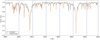 |
Fig. 2 Example of one spectral window used with different chunks of size 512 points indicated by the vertical dashed lines. |
3.4 Implementation
Regarding the implementation of the algorithm, we used TensorFlow v2, which is the premier open-source DL framework commonly available. It was developed and maintained by Google (Abadi 2015) and, since its direct usage can be challenging, a front-end framework named Keras was used as well (Chollet 2015).
The adoption of the TensorFlow framework for DL model creation enables the usage of accelerated hardware based on the Nvidia general-purpose graphics processing unit (GPU) cards, which outperforms the central processing unit computation (CPU) time by around a factor of twenty (Mittal & Vaishay 2019). In this application, we used GPU cards with 11 GB of RAM and 4352 computing cores. The training time for a model experiencing proper convergence depended on the training data size, but also on the architecture and number of epochs, and it varied between 45 min to several hours.
3.5 Different DL approaches
Different DL architectures were considered, some of them inspired by literature such as Sharma et al. (2019), StarNet (Kielty et al. 2018), and many other homemade architectures. To this end, a flexible python code was implemented where the topology for the convolutional structure and for the ANN layers were passed as parameters. In this way it was possible to distribute the computations among different computing nodes to increase parallelism, as well as keeping the software easy to maintain.
We used different spectral windows to derive the models. These were taken from Pass19 and are summarized in Table 2. For each window we considered a certain chunk size, which refers to the number of wavelengths points within the window. For some windows we used several chunk sizes, ranging from 256 to 4096 wavelength points, to explore the impact on the DL model and its predictions of the stellar parameters. Figure 2 shows an example for such a spectral window with different chunks marked. Three approaches were defined for the analysis as follows.
In approach A, we trained a DL model for one spectral window and predicted each stellar parameter individually. We modified the DL architecture by varying the number of convolutional, pooling, and ANN hidden layers. The different architectures ranged fromjust three convolutional layers with one max pooling layer, passing the flattened vector of features to an ANN having three hidden layers, to eight convolutional layers with and without intermediate pooling layers, both maximum and averaged. The feature vector was fed into an ANN having five hidden layers. The convolutional layers had implemented strategies from a few replications per layer and increasing as they moved over the layers and vice versa. In this way we investigated a possible difference in predictions depending on the architecture and spectral window used.
In approach B, different combinations of stellar parameters were analyzed. In this approach we derived a DL model for individual parameters, for both Teff and log g, and for [M/H] and v sin i, as well as for all the four parameters at the same time. Also here we determined predictions for the spectral windows in Table 2 and investigated different architectures. From this approach we see how a combined DL model impacted the stellar parameter predictions.
In approach C, we derived a DL model for each stellar parameter separately, but we combined spectral windows. For example, we combined the window starting at 8800 Å with the window starting at 12 510 Å to investigate the differences in the predictions when more spectral information is used. Also, other window couplings were analyzed, such as the combination of all the VIS channel windows, and all the NIR channel windows. Again, we determined DL models for different architectures.
As a summary, more than 2000 different DL models were created, and for selecting the most suitable ones, specific quality criteria were defined. Every model was applied across the test sample to estimate the quality of the forecast.This error threshold was used as quality criteria to select them for further usage over the observed spectra. The number of selected models, as well as the quality criteria, are shown in Table 3. The thresholds for defining a good quality model were adopted from the MSE criterion, ranging between 5 × 10⁻⁴ and 10−5. The aim was to produce a difference between real and estimated parameters less than the threshold presented in Table 3, independently of the value of the parameter. As an example, the prediction quality for the test dataset for some of the models is plotted in Fig. 3.
Quality criteria and number of suitable models trained from PHOENIX.
3.6 Application to CARMENES spectra
The synthetic gap is well-known in ML and refers to the differences in feature distributions between synthetic and observed data (Fabbro et al. 2018). Because the spectra are high-dimensional data with, in our case of synthetic spectra, up to 4096 flux values (i.e., dimensions) per spectral window, dimensional reduction is necessary to visualize the data in low-dimensional space. So we verified the synthetic gap by using a nonlinear projector from high-dimensional flux space into a two-dimensional space that preserved the local topology in order to understand similarities between PHOENIX and CARMENES spectra families. We decided to use the Uniform Manifold Approximation and Projection (UMAP; McInnes et al. 2018) with a metric that is a correlation between the spectra.
As can be seen in Fig. 4, only four of our investigated CARMENES spectra are close to the PHOENIX family (we plotted only a subset of the full PHOENIX grid for visibility). However, there is a significant set of CARMENES spectra (46 of 50) far away from the PHOENIX sample set used to train the DL, meaning that the flux features described by synthetic and observed spectra are significantly different. These large deviations can be explained by the synthetic gap. Due to the fact that synthetic spectra are not perfect, it is expected that the feature distributions of synthetic and observed spectra do not match completely, meaning that not all CARMENES spectra would fall right within the PHOENIX spectra in Fig. 4. However, such a big difference as observed here indicates significant differences between those two spectralfamilies and will transform into higher uncertainties on the stellar parameters derived using these synthetic spectra. To assess the possible relevance of the noise in this work we also added white Gaussian noise (S∕N = 50, 100, 150) to the PHOENIX set and compared the resulting UMAP projections. All the noisy PHOENIX spectra show a similar behavior as the noise-free spectra. In our case, an S/N of 150 served as a lower limit for the CARMENES spectra, since most of the observed spectra used in this work have higher S/N. The noisy PHOENIX spectra are not closer to the observed data in the UMAP, indicating that noise is not responsible for the synthetic gap. We note that, since this is a dimensional projection, the axes in Fig. 4 are not labeled, because they do not have a specific meaning here.
Being aware of such a gap, all accepted DL models from all three DL approaches described in Sect. 3.5 were applied to the 50 CARMENES spectra in order to estimate the stellar parameters. The parameter estimations from each DL model were collected and the probability density function was determined using the Kernel Density Estimate (KDE; Rosenblatt 1956; Parzen 1962). Based on such a density of probability function, the maximum was retained as the confident estimation for the parameter. This was done for each star and each stellar parameter separately. For providing the uncertainty for each star and parameter, the 1σ thresholds of the predictions were calculated. An example for a representative star is presented in Fig. 5. We included thestellar parameters derived by Pass19 for comparison.
4 Results and discussion
4.1 Performance of different DL approaches
When we apply our three DL approaches (A, B, C) to the PHOENIX test set, the predicted stellar parameters show that there is only little, ifany, influence from the DL architecture, as all of them are able to produce good quality DL models. There are also minimal differences when considering stellar parameters derived from different windows. Therefore, we conclude that there is enough spectral information to determine stellar parameters from any window, no matter what chunk size, since also no particular improvement is found when several windows were joined. The DL models are able to successfully predict individual stellar parameters. Obviously, this only refers to PHOENIX models and cannot be translated to the observed spectra because of the particular effects of the synthetic gap, and some other factors, such as measuring at specific wavelength ranges, telluric correction or different S/N. Nevertheless, when estimating the information content of stellar spectra from a purely theoretical point of view, similar results are obtained. For example, Hafner & Wehrse (1994) estimated to be able to retrieve more than ten parameters in a 1000 Å wide chunk in which the resolution is only a quarter of that of CARMENES. Therefore, a key lesson learned is related to the capability of the DL models to disentangle the specific effects found in the spectra by individual parameters even if a very small chunk of the spectrum is considered. Indeed, no particular attention to the DL architecture is required as all of those tested are capable of performing well.
During our tests, we also trained models predicting all four stellar parameters simultaneously, as it is done by The Cannon. However, we find that these models always give worse predictions, meaning higher validation errors, than individual ones. Therefore, we decided to estimate each stellar parameter individually.
4.2 Performance on CARMENES spectra
To address the second goal of this work (evaluate its application to observed spectra and the impact of the synthetic gap on the estimation of stellar parameters), we applied all trained models matching the quality criteria (see Table 3) to the observed CARMENES spectra, collected the results for each star, and drew statistical distributions for each parameter. This technique has the advantage of estimating uncertainties for each star and stellar parameter by calculating the 1σ deviations for each distribution.
Figure 6 shows a comparison between our estimated [M/H] and literature values, color-coded with our derived Teff. The degeneracy at low Teff and high [M/H] is evident in the top panel. This behavior was described already, for example in Passegger et al. (2018) and Pass19, who decided to break the degeneracy by determining log g independently from evolutionary models. In contrast to Pass19, who used the PARSEC v1.2S evolutionary models (Bressan et al. 2012; Chen et al. 2014, 2015; Tang et al. 2014) to derive log g depending on Teff and metallicity suggested by their downhill simplex method, we used the PARSEC library to constrain our synthetic model grid with which we trained our DL models. In this way we could remove stellar parameter combinations that are physically unrealistic for M dwarfs (i.e., they correspond to objects far away from the main sequence) and helped the DL to break the degeneracy. After applying this constraint, we tested our improved approach and trained new DL models for the wavelength window 8800–8835 Å, since this window shows the smallest MSE from all windows we investigated. Using the same quality criteria as presented in Table 3, we ended up with more than 200 accepted DL models for each stellar parameter. We find that constraining the synthetic model grid is indeed capable of breaking the observed parameter degeneracy (see bottom panel of Fig. 6). The hereby estimated stellar parameters, together with their uncertainties for the 50 CARMENES stars, are presented in Table 4.
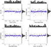 |
Fig. 3 Differences between input and output stellar parameters for the test set for an example DL model. The red line shows the average of all points and the blue shaded area is the 95% confidence region. |
4.3 Literature comparison
We compared our results to values from the literature, as shown in Fig. 7. To increase readability of the plots we present our errorbars in gray. We differentiated between several determination methods to visualize possible biases.
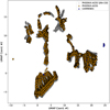 |
Fig. 4 Representative UMAP two-dimensional projection of CARMENES (blue) and PHOENIX spectra (S∕N = ∞ in yellow, S∕N = 150 in gray) built with the flux values from the 8800–8835 Å window. Only four CARMENES spectra show similarities with the PHOENIX feature distribution, while the rest are considerably different. Other spectral windows show a similar behavior. |
4.3.1 Effective temperature
The comparison of our estimated Teff to the following literature works is shown in the top left plot of Fig. 7. Synthetic model fits were performed by Pass19. As mentioned above, Gaidos & Mann (2014) and Mann et al. (2015) derived Teff from visual spectra using BT-Settl model fits. Our values are mostly consistent with these works within their errors. Spectral indices and pEWs were used by Rojas-Ayala et al. (2012), Maldonado et al. (2015), and Terrien et al. (2015). The latter study determined three different values of Teff and [M/H] in the J, H, and K bands. We took the values from the K band for comparison, because they report those values to be the most reliable. Gaidos & Mann (2014) calculated spectral curvature indices in the near-infrared for stars without visual spectra. In comparison, values from Rojas-Ayala et al. (2012) and Gaidos & Mann (2014) agree well with our results within their errors. We find no correlation with K-band Teff from Terrien et al. (2015), which basically form a straight line around 3300 K.
Houdebine et al. (2019) determined Teff using photometric colors. Their results are fairly consistent with our estimates in the temperature range below 3800 K, but tend to be considerably lower for higher temperatures. In general, there seems to be no bias regarding different determination methods, since all results follow the same pattern (except for Terrien et al. 2015).
There is one significant outlier, which is marked with a purple circle. This is GJ 87, for which we estimated a Teff of 3990 K, whereas several other works report temperatures 345 K cooler on average (Pass19: 3605 ± 54 K; Maldonado et al. 2015: 3562 ± 68 K; Gaidos & Mann 2014: 3783 ± 94 K; Mann et al. 2015: 3638 ± 62 K; Houdebine et al. 2019: 3645 ± 33 K). However, log g, [M/H], and v sin i (see below) are consistent with literature values within their errors. From the spectral type (M1.5 V) and its nearly solar metallicity (+0.07 dex), a temperature of around 3700 K would be more fitting (see Fig. 8 in Passegger et al. 2018), as reported in the literature. At this point we find no explanation for the large deviation in temperature, since this star is not young (e.g., Pass19 assumed 5 Gyr) and shows no magnetic activity.
Unfortunately, there are only three stars that we have in common with Antoniadis-Karnavas et al. (2020), who estimated their stellar parameters with the ML tool ODUSSEAS. For these stars we derived about 150 K higher temperatures than with ODUSSEAS. Also other literature values for these stars show higher temperatures and match better with our results.
4.3.2 Surface gravity
For log g (Fig. 7, top right), results from synthetic model fits come from Pass19. To obtain log g values for the other literature results, we calculated log g from the masses and radii the respective studies provide. Mann et al. (2015) determined the stellar mass from a mass-luminosity relation (Delfosse et al. 2000), and the stellar radius from employing the Stefan-Boltzmann law with Teff derived from BT-Settl fits and spectroscopically measured bolometric fluxes. Gaidos & Mann (2014) derived stellar masses in the same way as Mann et al. (2015). For the stellar radius they used the radius-temperature relationship from Mann et al. (2013b). Maldonado et al. (2015) determined stellar masses from empirical photometric relations and stellar radii from a mass-radius relationship involving interferometric measurements and eclipsing binaries. Their results are marked as “interferometric” in the plot. Although most values group along the 1:1 correlation and coincide with literature within their errors, we tentatively estimated lower log g compared to literature.
4.3.3 Metallicity
Since our [M/H] results directly translate into identical [Fe/H] values we can compare these with literature [Fe/H] results. Conversely, literature values of [Fe/H] are often interpreted as a proxy for [M/H]. The different measurements are distinguished in the bottom left plot of Fig. 7. As mentioned in Sect. 1, spectral indices, pEWs, and relations of atomic line strength to determine metallicity were used by Rojas-Ayala et al. (2012), Maldonado et al. (2015), Mann et al. (2015), and Gaidos & Mann (2014). Besides, Terrien et al. (2015) used both pEWs and spectral indices. Dittmann et al. (2016) derived [Fe/H] from color-magnitude metallicity relations. From these studies, only Rojas-Ayala et al. (2012), Terrien et al. (2015), and Pass19 provide [M/H], while all others claim [Fe/H].
All our metallicities seem to be constrained to the range 0.0 dex < [M/H] < +0.4 dex, in contrast to literature values, which lie in a wider range between –0.4 dex and +0.5 dex. Ignoring data points from Pass19 (i.e., “fit [M/H]”), all other literature values are more metal-poor compared to our estimations or, equivalently, our metallicities are too high. Similar to Teff, the three points of Antoniadis-Karnavas et al. (2020) lie in the lower range, presenting metallicities lower than ours and other literature, which might indicate that they tentatively derived too low values.
4.3.4 Rotational velocity
We compared our derived v sin i values with those from Reiners et al. (2018), who determined v sin i from CARMENES spectra as well. They used a cross-correlation method from several lines in spectral orders of low telluric contamination and high-S/N and provided errors only for v sin i > 2.0 km s−1, which is the lower detection limit with the CARMENES VIS spectral resolution. For our sample, these orders are located at wavelengths λ < 6850 Å. This might explain the differences that we get when we compare v sin i. The comparison in the bottom right plot of Fig. 7 shows that our DL approach slightly overestimates v sin i. However, the values are mostly consistent within their errors. There are several mechanism that can contribute to the broadening of spectral lines, such as magnetic activity, pressure broadening, and stellar rotation. For the first two the strength of the broadening depends on the properties of the considered atomic species. Only stellar rotation affects all lines in the same way, so it is appropriate to derive v sin i from several lines individually instead of only one small wavelength chunk, as it was done in this work. However, our focus lies toward stellar parameters Teff, log g, and [M/H].
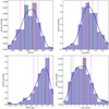 |
Fig. 5 DL estimations distribution for the CARMENES star GJ 169.1A (J04311+589). The KDE maximum (i.e., our adopted estimations, red lines) is shown together with the 1σ uncertainties (magenta lines) and results from Pass19 (green lines). The dark blue curve represents the Gaussian kernel density estimate. We used the default rules from the seaborn distplot function: Freedman-Diaconis’ (Freedman & Diaconis 1981) for the histogram bin width and Scott’s rule (Scott 1979) for the kernel size. |
4.4 Uncertainties, errors, and the synthetic gap
Error estimation is almost as challenging as stellar parameter determination itself. There are several ways that authors use to quantify errors in their works. In Pass19 the uncertainties were calculated by measuring the standard deviations of the differences between input and output stellar parameters for 1400 noise perturbed synthetic spectra. These uncertainties represent measurement errors of the method itself, but do not take into account the effects of the synthetic gap. For pEW methods, such as Maldonado et al. (2015), the measurement error in the stellar parameters is directly derived from uncertainties in the pEWs.
Mann et al. (2015) discussed different sources of uncertainties, taking into account measurement errors and errors from calibrations and photometric zero points. In other works (e.g., Houdebine et al. 2019), the error is stated as the difference between their results and the literature, which cannot be considered as a measurement or a systematic error.
Antoniadis-Karnavas et al. (2020) estimated their uncertainties by including the intrinsic uncertainties of the HARPS reference dataset, since these were used in the training process of the ML algorithm and, therefore, introduced noise. This approach can be seen as an attempt at error propagation and measured the influence on the predicted stellar parameters, meaning a unique global standard deviation for all the estimated parameters. Fabbro et al. (2018) estimated the prediction error for each stellar parameter by adding in quadrature statistical and intrinsic errors. The statistical error was computed from an error spectrum, giving an approximation of the error on the predicted output stellar parameter. The intrinsic error was empirically measured from a synthetic test sample.
What a real measurement should attempt to quantify is not only the measurement error but also any type of systematic error. In the case of spectral analyses, one source of systematic errors are the uncertainties inherent in the use of model atmospheres and the derived synthetic spectra. This becomes evident when comparing results of the post-2012 analyses cited in the introduction with those from the decades prior to the BT-Settl models. Important studies based on the previous model generations are, for example, Leggett et al. (2001, 2000) for the AMES-Dusty models (Allard et al. 2001), Gizis (1997) for the NextGen grid (Hauschildt et al. 1999), Leggett et al. (1996) and Jones et al. (1996) for the so called base grid (Allard & Hauschildt 1995), and Kirkpatrick et al. (1993) for the initial generation of this line of models (Allard 1990). Typically, the cited errors are smaller than the changes that happen when changing the set of model atmospheres. Obviously, the models have improved over the years, both in quality and the amount of details in the implemented physics. However, it is not guaranteed that future improvements in the models will not change the results significantly.
In this work, the synthetic gap gives us a valuable hint on the systematic error. Since it tells us how far away the models are from the observed spectra, the synthetic gap can serve two purposes. The obvious one is a call to improve the model atmospheres and synthetic spectra. Currently, we know which spectral chunks performed the best, that is that they show the smallest MSE during training. In the future we will investigate the variation of the synthetic gap over all the wavelength regions investigated by Passegger et al. (2018) and Pass19 (see Table 2), but this is beyond the scope of this paper. Identifying the reasons why some regions can be fitted well, yet showing a large synthetic gap, will point toward potential areas of improvement in the synthetic spectra. The other aspect is a warning toward those who use models: no synthetic spectrum is perfect even if a χ2-fit produces excellent agreement.
Another source of uncertainty is using a too small sample of reference stars for training. For example, Antoniadis-Karnavas et al. (2020) used only 65 stars in the training set. As discussed by Fabbro et al. (2018), it is necessary for a deep neural network to have a large training set that spans over the whole stellar parameter range. If there were only a few spectra available for a certain region of the parameter space, such as low temperatures, this would translate into less accurate estimations for stars in this region. This lack of information could become important when using observed spectra as a training set, since there might not be enough observations available to span the whole parameter space.
Furthermore, a possible misplacement of the continuum, especially for late-type stars, should be taken into account when estimating uncertainties. In our case, we used rather small wavelength ranges of a few 10 Å, and treated the continuum of the synthetic and observed spectra in the same way. As can be seen in Fig. 2, the GISIC algorithm did a good job in normalizing both spectra within this wavelength range. Therefore, we expect the uncertainty coming from a possible continuum misplacement of either spectrum to be negligible. However, because of the way we estimated our errors, those kind of uncertainties were already included.
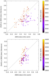 |
Fig. 6 Literature comparison for [M/H] with Teff color-coded, before (top) and after (bottom) applying the PARSEC constraint on the synthetic grid. |
5 Summary and conclusions
We present a deep learning neural network technique to estimate the stellar parameters Teff, log g, [M/H], and v sin i for M dwarfs from high-S/N, high-resolution, optical, and near-infrared spectroscopy. The DL models were trained with PHOENIX-ACES synthetic spectra, which has the advantage that it is possible to generate a sufficient number of spectra with known stellar parameters. We investigated different architectures and analyzed different spectral windows, which showed only negligible effects on the estimated stellar parameters. We find that all DL models produced only small training and validation errors, meaning that the DL models are able to estimate stellar parameters from synthetic spectra with high precision and accuracy. In other words, the information content of synthetic spectra (the determination of which is a fundamental astrophysical question) is sufficient to determine the four stellar parameters and is independent of the considered spectral windows.
After constraining the synthetic grid to the M-dwarf parameter space using PARSEC evolutionary models, we trained new DL models on one spectral window and tested their performance on 50 high-resolution CARMENES spectra. Although our results are in good agreement with the literature in most cases (especially for Teff and log g), significant deviations are found for the metallicity. We attribute those deviations to the synthetic gap, the difference of spectral feature distribution between synthetic and observed spectra.
To avoid uncertainties introduced by the synthetic gap, we conclude that it seems more practical to use observed spectra with known stellar parameters for training. However, the question arises where those “known” parameters come from, since they have to be derived by some method as well, which again introduces uncertainties. Also, it might be difficult to find a sufficient number of observed spectra covering the whole parameter range to properly train an accurate DL model.
A more detailed study is necessary to quantify the effect of the synthetic gap on stellar parameter determination and get to the bottom of its sources. For this study the main aim was to validate the DL method, which delivers satisfying results using synthetic models. However, shortcomings are identified when applying the trained DL models to observed spectra. Therefore, we will investigate the synthetic gap and its effect on [M/H] in more detail in a following study. We will also add noise to the synthetic spectra, which will help to simulate a more realistic setup in the training step, however, this will have no significant influence onthe synthetic gap. In summary, we present a method to derive stellar parameters with DL models trained on synthetic spectra and estimated the uncertainty related to the synthetic gap. This work should also be seen as aword of caution toward scientists employing synthetic spectra uncritically in their work, since even apparently perfect fits do not necessarily provide perfect results, which should be accounted for with larger error estimates.
Sample of CARMENES stars and derived parameters with 1 σ uncertainties.
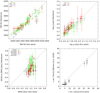 |
Fig. 7 Comparison of the results of this work with values from the literature. For better readability, the errorbars of this work are plotted in gray. Different symbols mark different determination methods of literature values. The ellipse in the top left panel marks the outlier star GJ 87 (J02123+035). Legend: fit (synthetic model fit): Passegger et al. (2019), Gaidos & Mann (2014) (Teff VIS), Mann et al. (2015) (Teff); spec (pEWs, spectral indices, spectroscopic relations): Rojas-Ayala et al. (2012); Maldonado et al. (2015), Gaidos & Mann (2014) (Teff NIR, log g, [Fe/H]), Mann et al. (2015) (log g, [Fe/H]), Terrien et al. (2015); ML: Antoniadis-Karnavas et al. (2020); phot (photometric): Dittmann et al. (2016); Houdebine et al. (2019); interfer (interferometry): Maldonado et al. (2015). |
Acknowledgements
We thank an anonymous referee for helpful comments that improved the quality of this paper. CARMENES is an instrument for the Centro Astronómico Hispano-Alemán de Calar Alto (CAHA, Almería, Spain). CARMENES is funded by the German Max-Planck-Gesellschaft (MPG), the Spanish Consejo Superior de Investigaciones Científicas(CSIC), European Regional Development Fund (ERDF) through projects FICTS-2011-02, ICTS-2017-07-CAHA-4, and CAHA16-CE-3978, and the members of the CARMENES Consortium (Max-Planck-Institut für Astronomie, Instituto de Astrofísicade Andalucía, Landessternwarte Königstuhl, Institut de Ciències de l’Espai, Insitut für Astrophysik Göttingen, Universidad Complutense de Madrid, Thüringer Landessternwarte Tautenburg, Instituto de Astrofísica de Canarias, Hamburger Sternwarte, Centro de Astrobiología and Centro Astronómico Hispano-Alemán), with additional contributions by the Spanish Ministry of Economy, the German Science Foundation through the Major Research Instrumentation Programme and DFG Research Unit FOR2544 “Blue Planets around Red Stars”, the Klaus Tschira Stiftung, the states of Baden-Württemberg and Niedersachsen, and by the Junta de Andalucía. We acknowledge financial support from NASA through grant NNX17AG24G, the Agencia Estatal de Investigación of the Ministerio de Ciencia through fellowship FPU15/01476, Innovación y Universidades and the ERDF through projects PID2019-109522GB-C51/2/3/4, AYA2016-79425-C3-1/2/3-P and AYA2018-84089, the Fundação para a Ciência e a Tecnologia through and ERDF through grants UID/FIS/04434/2019, UIDB/04434/2020 and UIDP/04434/2020, PTDC/FIS-AST/28953/2017, and COMPETE2020 - Programa Operacional Competitividade e Internacionalização POCI-01-0145-FEDER-028953.
References
- Abadi, M., e. a. 2015, TensorFlow: Large-Scale Machine Learning on Heterogeneous Systems, https://github.com/tensorflow/tensorflow, accessed: 2020-02-07 [Google Scholar]
- Abraham, S., Aniyan, A. K., Kembhavi, A. K., Philip, N. S., & Vaghmare, K. 2018, MNRAS, 477, 894 [Google Scholar]
- Allard, F. 1990, PhD thesis, Centre de Recherche Astrophysique de Lyon, France [Google Scholar]
- Allard, F., & Hauschildt, P. H. 1995, ApJ, 445, 433 [NASA ADS] [CrossRef] [Google Scholar]
- Allard, F., Hauschildt, P. H., Alexander, D. R., Tamanai, A., & Schweitzer, A. 2001, ApJ, 556, 357 [NASA ADS] [CrossRef] [Google Scholar]
- Allard, F., Homeier, D., & Freytag, B. 2011, ASP Conf. Ser., 448, 91 [NASA ADS] [Google Scholar]
- Allard, F., Homeier, D., & Freytag, B. 2012, Phil. Trans. R. Soc. London Ser. A, 370, 2765 [Google Scholar]
- Allard, F., Homeier, D., Freytag, B., et al. 2013, Mem. Soc. Astron. It. Suppl., 24, 128 [Google Scholar]
- Alvarez, R., & Plez, B. 1998, A&A, 330, 1109 [NASA ADS] [Google Scholar]
- Anthony, M., & Bartlett, P. L. 2009, Neural Network Learning: Theoretical Foundations (Cambridge: Cambridge University Press) [Google Scholar]
- Antoniadis-Karnavas, A., Sousa, S. G., Delgado-Mena, E., et al. 2020, A&A, 636, A9 [CrossRef] [EDP Sciences] [Google Scholar]
- Bailer-Jones, C. A. L., Irwin, M., Gilmore, G., & von Hippel, T. 1997, MNRAS, 292, 157 [NASA ADS] [Google Scholar]
- Bean, J. L., Benedict, G. F., & Endl, M. 2006, ApJ, 653, L65 [NASA ADS] [CrossRef] [Google Scholar]
- Birky, J. L., Aganze, C., Burgasser, A. J., et al. 2017, AAS Meeting Abstracts, 229, 240.18 [NASA ADS] [Google Scholar]
- Birky, J., Hogg, D. W., Mann, A. W., & Burgasser, A. 2020, ApJ, 892, 31 [CrossRef] [Google Scholar]
- Bonfils, X., Delfosse, X., Udry, S., et al. 2005, A&A, 442, 635 [NASA ADS] [CrossRef] [EDP Sciences] [Google Scholar]
- Boyajian, T. S., von Braun, K., van Belle, G., et al. 2012, ApJ, 757, 112 [NASA ADS] [CrossRef] [Google Scholar]
- Bressan, A., Marigo, P., Girardi, L., et al. 2012, MNRAS, 427, 127 [NASA ADS] [CrossRef] [Google Scholar]
- Caballero, J. A., Guàrdia, J., López del Fresno, M., et al. 2016, Proc. SPIE, 9910, 99100E [Google Scholar]
- Casagrande, L., Flynn, C., & Bessell, M. 2008, MNRAS, 389, 585 [NASA ADS] [CrossRef] [MathSciNet] [Google Scholar]
- Casey, A. R., Hogg, D. W., Ness, M., et al. 2016, arXiv e-prints, [arXiv:1603.03040] [Google Scholar]
- Chen, Y., Girardi, L., Bressan, A., et al. 2014, MNRAS, 444, 2525 [NASA ADS] [CrossRef] [Google Scholar]
- Chen, Y., Bressan, A., Girardi, L., et al. 2015, MNRAS, 452, 1068 [NASA ADS] [CrossRef] [Google Scholar]
- Chollet, F. 2015, KERAS, https://github.com/keras-team/keras, accessed: 2020-02-07 [Google Scholar]
- Czesla, S., Schröter, S., Schneider, C. P., et al. 2019, PyA: Python astronomy-related packages [Google Scholar]
- Delfosse, X., Forveille, T., Ségransan, D., et al. 2000, A&A, 364, 217 [NASA ADS] [Google Scholar]
- Demory, B. O., Ségransan, D., Forveille, T., et al. 2009, A&A, 505, 205 [NASA ADS] [CrossRef] [EDP Sciences] [Google Scholar]
- Dhital, S., West, A. A., Stassun, K. G., et al. 2012, AJ, 143, 67 [NASA ADS] [CrossRef] [Google Scholar]
- Dieleman, S., Willett, K. W., & Dambre, J. 2015, MNRAS, 450, 1441 [NASA ADS] [CrossRef] [Google Scholar]
- Dittmann, J. A., Irwin, J. M., Charbonneau, D., & Newton, E. R. 2016, ApJ, 818, 153 [NASA ADS] [CrossRef] [Google Scholar]
- Fabbro, S., Venn, K. A., O’Briain, T., et al. 2018, MNRAS, 475, 2978 [NASA ADS] [CrossRef] [Google Scholar]
- Figueira, P., Adibekyan, V. Z., Oshagh, M., et al. 2016, A&A, 586, A101 [NASA ADS] [CrossRef] [EDP Sciences] [Google Scholar]
- Freedman, D., & Diaconis, P. 1981, Zeitschrift für Wahrscheinlichkeitstheorie und Verwandte Gebiete, 57, 453 [Google Scholar]
- Gaidos, E., & Mann, A. W. 2014, ApJ, 791, 54 [NASA ADS] [CrossRef] [Google Scholar]
- Gizis, J. E. 1997, AJ, 113, 806 [NASA ADS] [CrossRef] [Google Scholar]
- Gong, B., & Ordieres-Meré, J. 2016, Environ. Modell. Softw., 84, 290 [CrossRef] [Google Scholar]
- González-Marcos, A., Ordieres-Meré, J., Alba-Elías, F., de Pisón, F. J. M., & Castejón-Limas, M. 2013, Ironmaking Steelmaking, 41, 262 [CrossRef] [Google Scholar]
- González-Marcos, A., Sarro, L. M., Ordieres-Meré, J., & Bello-García, A. 2017, MNRAS, 465, 4556 [CrossRef] [Google Scholar]
- Gulati, R. K., Gupta, R., Gothoskar, P., & Khobragade, S. 1994, ApJ, 426, 340 [Google Scholar]
- Gustafsson, B., Edvardsson, B., Eriksson, K., et al. 2008, A&A, 486, 951 [NASA ADS] [CrossRef] [EDP Sciences] [Google Scholar]
- Hafner, M., & Wehrse, R. 1994, A&A, 282, 874 [Google Scholar]
- Hartman, J. D., Bayliss, D., Brahm, R., et al. 2015, AJ, 149, 166 [NASA ADS] [CrossRef] [Google Scholar]
- Hauschildt, P. H. 1992, J. Quant. Spectr. Rad. Transf., 47, 433 [Google Scholar]
- Hauschildt, P. H. 1993, J. Quant. Spectr. Rad. Transf., 50, 301 [Google Scholar]
- Hauschildt, P. H., Allard, F., & Baron, E. 1999, ApJ, 512, 377 [NASA ADS] [CrossRef] [Google Scholar]
- Hauschildt, P. H., & Baron, E. 1999, J. Comput. Appl. Math., 109, 41 [NASA ADS] [CrossRef] [Google Scholar]
- He, W., & Zhao, G. 2019, Res. A&A, 19, 140 [Google Scholar]
- Hon, M., Stello, D., & Yu, J. 2017, MNRAS, 469, 4578 [Google Scholar]
- Houdebine, É. R., Mullan, D. J., Doyle, J. G., et al. 2019, AJ, 158, 56 [CrossRef] [Google Scholar]
- Husser, T.-O., Wende-von Berg, S., Dreizler, S., et al. 2013, A&A, 553, A6 [NASA ADS] [CrossRef] [EDP Sciences] [Google Scholar]
- Johnson, J. A., & Apps, K. 2009, ApJ, 699, 933 [NASA ADS] [CrossRef] [Google Scholar]
- Johnson, J. A., Gazak, J. Z., Apps, K., et al. 2012, AJ, 143, 111 [NASA ADS] [CrossRef] [Google Scholar]
- Johnson, S. G., Cervellino, A., Wuttke, J. 2019, libcerf, numeric library for complex error functions, version 1.13, https://jugit.fz-juelich.de/mlz/libcerf [Google Scholar]
- Jones, H. R. A., Longmore, A. J., Allard, F., & Hauschildt, P. H. 1996, MNRAS, 280, 77 [NASA ADS] [CrossRef] [Google Scholar]
- Kausch, W., Noll, S., Smette, A., et al. 2014, ASP Conf. Ser., 485, 403 [NASA ADS] [Google Scholar]
- Khata, D., Mondal, S., Das, R., Ghosh, S., & Ghosh, S. 2020, MNRAS, 493, 4533 [Google Scholar]
- Kielty, C. L., Bialek, S., Fabbro, S., et al. 2018, Int. Soc. Opt. Photon., 10707, 107072W [Google Scholar]
- Kirkpatrick, J. D., Kelly, D. M., Rieke, G. H., et al. 1993, ApJ, 402, 643 [NASA ADS] [CrossRef] [Google Scholar]
- Kuznetsov, M. K., del Burgo, C., Pavlenko, Y. V., & Frith, J. 2019, ApJ, 878, 134 [Google Scholar]
- LeCun, Y., Bengio, Y., & Hinton, G. 2015, Nature, 521, 436 [NASA ADS] [CrossRef] [PubMed] [Google Scholar]
- Leggett, S. K., Allard, F., Berriman, G., Dahn, C. C., & Hauschildt, P. H. 1996, ApJS, 104, 117 [NASA ADS] [CrossRef] [EDP Sciences] [Google Scholar]
- Leggett, S. K., Allard, F., Dahn, C., et al. 2000, ApJ, 535, 965 [NASA ADS] [CrossRef] [Google Scholar]
- Leggett, S. K., Allard, F., Geballe, T. R., Hauschildt, P. H., & Schweitzer, A. 2001, ApJ, 548, 908 [NASA ADS] [CrossRef] [Google Scholar]
- Leung, H. W., & Bovy, J. 2019, MNRAS, 483, 3255 [NASA ADS] [Google Scholar]
- Li, X.-R., Pan, R.-Y., & Duan, F.-Q. 2017, Res. A&A, 17, 036 [Google Scholar]
- Mahabal, A., Sheth, K., Gieseke, F., et al. 2017, ArXiv e-prints, [arXiv:1709.06257] [Google Scholar]
- Maldonado, J., Affer, L., Micela, G., et al. 2015, A&A, 577, A132 [NASA ADS] [CrossRef] [EDP Sciences] [Google Scholar]
- Mann, A. W., Brewer, J. M., Gaidos, E., Lépine, S., & Hilton, E. J. 2013a, AJ, 145, 52 [NASA ADS] [CrossRef] [Google Scholar]
- Mann, A. W., Gaidos, E., & Ansdell, M. 2013b, ApJ, 779, 188 [NASA ADS] [CrossRef] [Google Scholar]
- Mann, A. W., Deacon, N. R., Gaidos, E., et al. 2014, AJ, 147, 160 [NASA ADS] [CrossRef] [Google Scholar]
- Mann, A. W., Feiden, G. A., Gaidos, E., Boyajian, T., & von Braun, K. 2015, ApJ, 804, 64 [CrossRef] [Google Scholar]
- McCarthy, J., & Hayes, P. J. 1981, in Readings in Artificial Intelligence (Amsterdam: Elsevier), 431 [CrossRef] [Google Scholar]
- McInnes, L., Healy, J., Saul, N., & Grossberger, L. 2018, J. Open Source Softw., 3, 861 [Google Scholar]
- Meyer, M. 2017, PhD thesis, Universität Hamburg, Germany [Google Scholar]
- Mittal, S., & Vaishay, S. 2019, J. Syst. Archit., 99, 101635 [CrossRef] [Google Scholar]
- Montes, D., González-Peinado, R., Tabernero, H. M., et al. 2018, MNRAS, 479, 1332 [Google Scholar]
- Nagel, E., Czesla, S., Kaminski, A., et al. 2020, A&A, submitted [Google Scholar]
- Nemravová, J. A., Harmanec, P., Brož, M., et al. 2016, A&A, 594, A55 [NASA ADS] [CrossRef] [EDP Sciences] [Google Scholar]
- Ness, M., Hogg, D. W., Rix, H. W., Ho, A. Y. Q., & Zasowski, G. 2015, ApJ, 808, 16 [NASA ADS] [CrossRef] [Google Scholar]
- Neves, V., Bonfils, X., Santos, N. C., et al. 2012, A&A, 538, A25 [NASA ADS] [CrossRef] [EDP Sciences] [Google Scholar]
- Neves, V., Bonfils, X., Santos, N. C., et al. 2013, A&A, 551, A36 [NASA ADS] [CrossRef] [EDP Sciences] [Google Scholar]
- Neves, V., Bonfils, X., Santos, N. C., et al. 2014, A&A, 568, A121 [NASA ADS] [CrossRef] [EDP Sciences] [Google Scholar]
- Newton, E. R., Charbonneau, D., Irwin, J., et al. 2014, AJ, 147, 20 [NASA ADS] [CrossRef] [Google Scholar]
- Newton, E. R., Charbonneau, D., Irwin, J., & Mann, A. W. 2015, ApJ, 800, 85 [NASA ADS] [CrossRef] [Google Scholar]
- Önehag, A., Heiter, U., Gustafsson, B., et al. 2012, A&A, 542, A33 [NASA ADS] [CrossRef] [EDP Sciences] [Google Scholar]
- Paletou, F., Gebran, M., Houdebine, E. R., & Watson, V. 2015, A&A, 580, A78 [NASA ADS] [CrossRef] [EDP Sciences] [Google Scholar]
- Parzen, E. 1962, Ann. Math. Stat., 33, 1065 [NASA ADS] [CrossRef] [MathSciNet] [Google Scholar]
- Passegger, V. M., Reiners, A., Jeffers, S. V., et al. 2018, A&A, 615, A6 [NASA ADS] [CrossRef] [EDP Sciences] [Google Scholar]
- Passegger, V. M., Schweitzer, A., Shulyak, D., et al. 2019, A&A, 627, A161 [NASA ADS] [CrossRef] [EDP Sciences] [Google Scholar]
- Petersen, P., & Voigtlaender, F. 2018, Neural Netw., 108, 296 [CrossRef] [Google Scholar]
- Plez, B. 2012, Astrophysics Source Code Library [record ascl:1205.004] [Google Scholar]
- Quirrenbach, A., Amado, P. J., Ribas, I., et al. 2018, SPIE Conf. Ser., 10702, 107020W [Google Scholar]
- Rajpurohit, A. S., Allard, F., Rajpurohit, S., et al. 2018, A&A, 620, A180 [NASA ADS] [CrossRef] [EDP Sciences] [Google Scholar]
- Reiners, A., Zechmeister, M., Caballero, J. A., et al. 2018, A&A, 612, A49 [NASA ADS] [CrossRef] [EDP Sciences] [Google Scholar]
- Rodríguez Martínez, R., Ballard, S., Mayo, A., et al. 2019, AJ, 158, 135 [CrossRef] [Google Scholar]
- Rojas-Ayala, B., Covey, K. R., Muirhead, P. S., & Lloyd, J. P. 2010, ApJ, 720, L113 [NASA ADS] [CrossRef] [Google Scholar]
- Rojas-Ayala, B., Covey, K. R., Muirhead, P. S., & Lloyd, J. P. 2012, ApJ, 748, 93 [NASA ADS] [CrossRef] [Google Scholar]
- Rosenblatt, M. 1956, Ann. Math. Stat., 27, 832 [CrossRef] [MathSciNet] [Google Scholar]
- Sarro, L. M., Ordieres-Meré, J., Bello-García, A., González-Marcos, A., & Solano, E. 2018, MNRAS, 476, 1120 [Google Scholar]
- Schlaufman, K. C., & Laughlin, G. 2010, A&A, 519, A105 [NASA ADS] [CrossRef] [EDP Sciences] [Google Scholar]
- Schmidhuber, J. 2015, Neural Netw., 61, 85 [Google Scholar]
- Schweitzer, A., Passegger, V. M., Cifuentes, C., et al. 2019, A&A, 625, A68 [NASA ADS] [CrossRef] [EDP Sciences] [Google Scholar]
- Scott, D. W. 1979, Biometrika, 66, 605 [CrossRef] [MathSciNet] [Google Scholar]
- Ségransan, D., Kervella, P., Forveille, T., & Queloz, D. 2003, A&A, 397, L5 [NASA ADS] [CrossRef] [EDP Sciences] [Google Scholar]
- Shallue, C. J.,& Vanderburg, A. 2018, AJ, 155, 94 [NASA ADS] [CrossRef] [Google Scholar]
- Sharma, K., Kembhavi, A., Kembhavi, A., et al. 2019, MNRAS, 491, 2280 [Google Scholar]
- Shetrone, M., Bizyaev, D., Lawler, J. E., et al. 2015, ApJS, 221, 24 [Google Scholar]
- Singh, H. P., Gulati, R. K., & Gupta, R. 1998, MNRAS, 295, 312 [NASA ADS] [CrossRef] [Google Scholar]
- Smette, A., Sana, H., Noll, S., et al. 2015, A&A, 576, A77 [NASA ADS] [CrossRef] [EDP Sciences] [Google Scholar]
- Sneden, C. A. 1973, PhD thesis, The University of Texas at Austin, USA [Google Scholar]
- Souto, D., Cunha, K., García-Hernández, D. A., et al. 2017, ApJ, 835, 239 [NASA ADS] [CrossRef] [Google Scholar]
- Souto, D., Unterborn, C. T., Smith, V. V., et al. 2018, ApJ, 860, L15 [NASA ADS] [CrossRef] [Google Scholar]
- Souto, D., Cunha, K., Smith, V. V., et al. 2020, ApJ, 890, 133 [CrossRef] [Google Scholar]
- Steels, L. 1993, Artif. Life, 1, 75 [CrossRef] [Google Scholar]
- Tang, J., Bressan, A., Rosenfield, P., et al. 2014, MNRAS, 445, 4287 [NASA ADS] [CrossRef] [Google Scholar]
- Terrien, R. C., Mahadevan, S., Bender, C. F., et al. 2012, ApJ, 747, L38 [NASA ADS] [CrossRef] [Google Scholar]
- Terrien, R. C., Mahadevan, S., Bender, C. F., Deshpande, R., & Robertson, P. 2015, ApJ, 802, L10 [NASA ADS] [CrossRef] [Google Scholar]
- Valenti, J. A., & Fischer, D. A. 2005, ApJS, 159, 141 [NASA ADS] [CrossRef] [MathSciNet] [Google Scholar]
- Valenti, J. A., & Piskunov, N. 1996, A&AS, 118, 595 [NASA ADS] [CrossRef] [EDP Sciences] [Google Scholar]
- Veyette, M. J., Muirhead, P. S., Mann, A. W., et al. 2017, ApJ, 851, 26 [NASA ADS] [CrossRef] [Google Scholar]
- von Braun, K., Boyajian, T. S., van Belle, G. T., et al. 2014, MNRAS, 438, 2413 [NASA ADS] [CrossRef] [Google Scholar]
- von Hippel, T., Storrie-Lombardi, L. J., Storrie-Lombardi, M. C., & Irwin, M. J. 1994, MNRAS, 269, 97 [NASA ADS] [Google Scholar]
- Whitten, D. D., Placco, V. M., Beers, T. C., et al. 2019, A&A, 622, A182 [NASA ADS] [CrossRef] [EDP Sciences] [Google Scholar]
- Woolf, V. M., & Wallerstein, G. 2006, PASP, 118, 218 [NASA ADS] [CrossRef] [Google Scholar]
- Wu, C., Wong, O. I., Rudnick, L., et al. 2018, MNRAS, 482, 1211 [Google Scholar]
- Zboril, M., & Byrne, P. B. 1998, MNRAS, 299, 753 [NASA ADS] [CrossRef] [Google Scholar]
- Zboril, M., Byrne, P. B., & Rolleston, W. R. J. 1998, MNRAS, 301, 1104 [Google Scholar]
- Zechmeister, M., Anglada-Escudé, G., & Reiners, A. 2014, A&A, 561, A59 [NASA ADS] [CrossRef] [EDP Sciences] [Google Scholar]
- Zechmeister, M., Reiners, A., Amado, P. J., et al. 2018, A&A, 609, A12 [CrossRef] [Google Scholar]
- Zhang, G., Patuwo, B. E., & Hu, M. Y. 1998, Int. J. Forecasting, 14, 35 [Google Scholar]
- Zheng, X., Wang, M., & Ordieres-Meré, J. 2018, Sensors, 18, 2146 [Google Scholar]
Calar Alto high-Resolution search for M dwarfs with Exo-earths with Near-infrared and optical Échelle Spectrographs, http://carmenes.caha.es
All Tables
All Figures
|
Fig. 1 Generic architecture for DL models in this work. |
| In the text | |
|
Fig. 2 Example of one spectral window used with different chunks of size 512 points indicated by the vertical dashed lines. |
| In the text | |
|
Fig. 3 Differences between input and output stellar parameters for the test set for an example DL model. The red line shows the average of all points and the blue shaded area is the 95% confidence region. |
| In the text | |
|
Fig. 4 Representative UMAP two-dimensional projection of CARMENES (blue) and PHOENIX spectra (S∕N = ∞ in yellow, S∕N = 150 in gray) built with the flux values from the 8800–8835 Å window. Only four CARMENES spectra show similarities with the PHOENIX feature distribution, while the rest are considerably different. Other spectral windows show a similar behavior. |
| In the text | |
|
Fig. 5 DL estimations distribution for the CARMENES star GJ 169.1A (J04311+589). The KDE maximum (i.e., our adopted estimations, red lines) is shown together with the 1σ uncertainties (magenta lines) and results from Pass19 (green lines). The dark blue curve represents the Gaussian kernel density estimate. We used the default rules from the seaborn distplot function: Freedman-Diaconis’ (Freedman & Diaconis 1981) for the histogram bin width and Scott’s rule (Scott 1979) for the kernel size. |
| In the text | |
|
Fig. 6 Literature comparison for [M/H] with Teff color-coded, before (top) and after (bottom) applying the PARSEC constraint on the synthetic grid. |
| In the text | |
|
Fig. 7 Comparison of the results of this work with values from the literature. For better readability, the errorbars of this work are plotted in gray. Different symbols mark different determination methods of literature values. The ellipse in the top left panel marks the outlier star GJ 87 (J02123+035). Legend: fit (synthetic model fit): Passegger et al. (2019), Gaidos & Mann (2014) (Teff VIS), Mann et al. (2015) (Teff); spec (pEWs, spectral indices, spectroscopic relations): Rojas-Ayala et al. (2012); Maldonado et al. (2015), Gaidos & Mann (2014) (Teff NIR, log g, [Fe/H]), Mann et al. (2015) (log g, [Fe/H]), Terrien et al. (2015); ML: Antoniadis-Karnavas et al. (2020); phot (photometric): Dittmann et al. (2016); Houdebine et al. (2019); interfer (interferometry): Maldonado et al. (2015). |
| In the text | |
Current usage metrics show cumulative count of Article Views (full-text article views including HTML views, PDF and ePub downloads, according to the available data) and Abstracts Views on Vision4Press platform.
Data correspond to usage on the plateform after 2015. The current usage metrics is available 48-96 hours after online publication and is updated daily on week days.
Initial download of the metrics may take a while.