| Issue |
A&A
Volume 642, October 2020
|
|
|---|---|---|
| Article Number | A80 | |
| Number of page(s) | 29 | |
| Section | Planets and planetary systems | |
| DOI | https://doi.org/10.1051/0004-6361/202038246 | |
| Published online | 06 October 2020 | |
Ground-based visible spectroscopy of asteroids to support the development of an unsupervised Gaia asteroid taxonomy
1
INAF, Osservatorio Astrofisico di Torino,
Via Osservatorio 20,
10025
Pino Torinese, Italy
e-mail: This email address is being protected from spambots. You need JavaScript enabled to view it.
2
Université de la Côte d’Azur – Observatoire de la Côte d’Azur, CNRS, Laboratoire Lagrange, Campus Valrose Nice,
Nice Cedex 4, France
e-mail: This email address is being protected from spambots. You need JavaScript enabled to view it.
3
Université Côte d’Azur, Observatoire de la Côte d’Azur, CNRS, Laboratoire Lagrange, Boulevard de l’Observatoire, CS34229,
06304
Nice Cedex 4,
France
e-mail: This email address is being protected from spambots. You need JavaScript enabled to view it.
4
Planetary Science Institute,
Tucson,
AZ, USA
Received:
24
April
2020
Accepted:
29
July
2020
Abstract
Context. The Gaia mission of the European Space Agency is measuring reflectance spectra of a number to the order of 105 small Solar System objects. A first sample will be published in the Gaia Data Release scheduled for 2021.
Aims. The aim of our work was to test the procedure developed to obtain taxonomic classifications for asteroids based only on Gaia spectroscopic data.
Methods. We used asteroid spectra obtained using the DOLORES (Device Optimised for the LOw RESolution) instrument, a low-resolution spectrograph and camera installed at the Nasmyth B focus of the Telescopio Nazionale Galileo. Because these spectra have a higher spectral resolution than that typical of the Gaia spectra, we resampled them to more closely match the expected Gaia spectral resolution. We then developed a cloning algorithm to build a database of asteroid spectra belonging to a variety of taxonomic classes, starting from a set of 33 prototypes chosen from the 50 asteroids in our observing campaign. We used them to generate a simulated population of 10 000 representative asteroid spectra and employed them as the input to the algorithm for taxonomic classification developed to analyze Gaia asteroid spectra.
Results. Using the simulated population of 10 000 representative asteroid spectra in the algorithm to be used to produce the Gaia asteroid taxonomy at the end of the mission, we found 12 distinct taxonomic classes. Two of them, with 53% of the sample, are dominant. At the other extreme are three classes each with <1% of the sample, and these consist of the previously known rare classes A, D/Ld, and V; 99.1% of the simulated population fall into a single class.
Conclusions. We demonstrated the robustness of our algorithm for taxonomic classification by using a sample of simulated asteroid spectra fully representative of what is expected to be in the Gaia spectroscopic data catalogue for asteroids. Increasingly larger data sets will become available as soon as they are published in the future Gaia data releases, with the next one coming in 2021. This will be exploited to develop a correspondingly improved taxonomy, likely with minor tweaks to the algorithm described here, as suggested by the results of this preliminary analysis.
Key words: minor planets, asteroids: general / techniques: spectroscopic
© ESO 2020
1 Introduction
Among the many results that are expected from the Gaia mission of the European Space Agency, one is the measurement of the reflectance spectra for a large number (to the order of 105: see Tanga & Mignard 2012 and Delbò et al. 2012) of small Solar System bodies, which are mostly main-belt asteroids. These spectra are expected to produce a substantial advancement in asteroid science. They will be analysed to derive a new taxonomic classification based on this large data set, to obtain an improved understanding of the distribution of different taxonomic classes as a function of heliocentric distance, and to better define the membership of asteroid dynamical families, just to mention two applications. For a review of the general topic of asteroid spectroscopy and its implications, see DeMeo et al. (2015). A preliminary sample of Gaia asteroid reflectance spectra will be published in the next Gaia Data Release 3, planned for 2021. For the first time, therefore, the techniques developed to optimise the treatment of Gaia spectroscopic measurements of small Solar System objects will be applied to real data.
In this paper, we test the procedures which will be used to derive a taxonomic classification system based on the large amount of asteroid spectra provided by Gaia. Our tests are based on the results of a spectroscopic campaign that we carried out at the Telescopio Nazionale Galileo (TNG) in La Palma. For the purposes of taxonomic classification, we developed a cloning algorithm to build a large database of asteroid spectra belonging to a variety of taxonomic classes, starting from a limited set of prototypes chosen among the targets of our observing campaign.
Two critical features of Gaia observations of Solar System objects must be taken into account. First, Gaia covers a comparatively wide spectral interval of visible wavelengths, from blue to red, nominally between 0.330 and 1.050 μm (Gaia Collaboration 2016). This includes the blue-violet end of asteroid reflectance spectra, a region that has been substantially lost in modern CCD-based asteroid spectroscopic surveys. We can expect that in cases of faint asteroids (beyond some limiting magnitude that will be determined when the data becomes available) Gaia will collect signals that tend to be quite weak shortward of about 0.4 μm. In spite of this possible limitation, however, we expect a substantial improvement with respect to the majority of modern ground-based spectroscopic surveys of small bodies.
The behaviour of the reflectance spectrum at short wavelengths is very important. In the 1970s and 1980s, when spectro-photometric data were obtained using photoelectric photomultipliers, it made it possible to discriminateamong different taxonomic classes and sub-classes mostly including primitive, low-albedo objects, as shown bypioneering UBV observations (Bowell & Lumme 1979; Zellner 1979). A classic example is the old F class, which was first defined by Gradie & Tedesco (1982). This class, characterised by a flat behaviour down to the blue and UV spectral region, was later lost in the most recent SMASS (Bus & Binzel 2002b), S3 OS2 (Lazzaro et al. 2004), and DeMeo (DeMeo et al. 2009) spectroscopic surveys, due to insufficient coverage of the blue region of the spectrum by the CCD detectors used in modern asteroid spectroscopic surveys. However, polarimetric data confirm that the old F-class asteroids really form a distinct class, which is characterised by a well-defined and unusual polarimetric behaviour and includes some objects known to exhibit some kind of cometary activity, including (4015) Wilson Harrington and (101955) Bennu, the target of the OSIRIS-REx space mission (Belskaya et al. 2005, 2017; Cellino et al. 2015a, 2018; Devogèle et al. 2018a).
Another important fact to be taken into account is that Gaia observes main-belt asteroids at comparatively large phase angles1, mostly between 10° and 35°. There are reasons to expect that this can affect the resulting reflectance spectra. A phase-dependent effect of asteroid spectral reddening has been discussed by many authors in the past (Millis et al. 1976; Lumme & Bowell 1981; Nathues 2010; Reddy et al. 2012, 2015; Sanchez et al. 2012). According to Carvano & Davalos (2015), the spectral slope, namely the (mostly linear) change of reflectance from blue to red, tends generally to increase for increasing phase angle. The above authors, however, found that the variation of spectral slope is also affected by other properties of the objects, including shape and surface scattering properties, which can in some cases compete against reddening due to the phase angle. The behaviour of the spectral slope as a function of phase angle is therefore a complicated interplay of different mechanisms and cannot be easily predicted. A reddening occurs in most cases, but its amplitude can vary much among different objects.
We note that phase angle effects are even more important in the case of near-Earth asteroids (NEA) simply because, for geometric reasons, they can reach higher phase angles when seen at relatively small distances by a ground-based (or L2-based) observer (see, for a review, Binzel et al. 2019). In this paper, however, we limit our analysis to the case of main-belt (plus a couple of Jupiter Trojans) asteroids, because they constitute the vast majority of small bodies observed by Gaia. For them, phase angle effects are expected to be less significant than in the case of NEAs, but not negligible.
For the above reasons, in our analysis we did not simply use existing and publicly available asteroid spectra published as a result of important spectroscopic surveys at visible wavelengths, including Lazzaro et al. (2004) for main-belt asteroids, Lazzarin et al. (2004), for NEAs, in addition to the SMASS survey and the visible + near-IR DeMeo survey, of which the results are extensively used in this paper. Most published spectra, as a rule, do not cover the full interval of wavelengths that are covered by Gaia, and/or are the results of observations obtained at low phase angles. We therefore decided to carry out new observations of a large variety of objects, to obtain spectra covering, as much as possible, the same wavelength interval covered by Gaia, and to preferentially observe our targets at large phase angles. We chose our target list in such a way as to include members of as many taxonomic classes as possible, since taxonomic classes are defined based on differences in spectral reflectance. Our goal was to use the new spectra as constraints to validate and test the algorithm of taxonomic classification specifically developed for Gaia.
We stress that the purpose of our observations was not to obtain extremely accurate reflectance spectra to be used for the purposes of mineralogical interpretation through the analysis of detailed spectral features. As explained in the following sections, our analysis includes some modelling of realistic effects of spectral heterogeneity among objects sharing the same taxonomic classification. It is known, in fact, that the reflectance spectra of objects belonging to a same taxonomic class are not identical, but they exhibit variations within the same class, due both to slight differences in surface properties, but also to unavoidable observation errors, most often affecting the spectral slope, see Bus & Binzel (2002a). In this classical paper, the authors noted that the source of sporadic changes in spectral slope, which are occasionally measured, can hardly be determined. Their conclusion was as follows: “As spectral observations become more common, and asteroids are re-observed by different observers, we suggest that offsets in the overall slopes of spectra may be routinely seen. Care must therefore be taken to separate these random offsets from potentially real variations in the spectra due to physically meaningful effects such as phase reddening or compositional heterogeneity over the surface of an asteroid.”.
Moreover, we note that all methods of taxonomic classification have to face the problem of putting boundaries in the spectral properties adopted to divide large numbers of spectra into separate classes (Bus 1999; Bus & Binzel 2002b).
As a consequence, we did not limit ourselves to the analysis of only a small number of newly observed spectra, but instead used the objects included in our limited data set, characterised by the fact of including the blue spectral region, as representative end-members of a larger variety of possible situations expected to be encountered in Gaia data, as we explain in the next section.
In Sect. 2, we describe and present the results of our observations, including a description of some problems we encountered. A discretisation of our spectroscopic data to make them suitable to be used as prototypes of the expected spectroscopic signals obtained by Gaia is described in Sect. 3. In Sect. 4, we describe how we used our limited ground-based sample to build a much larger set of realistic spectral “clones”, needed as input to the algorithm for taxonomic classification that we developed for the analysis of large numbers of Gaia spectroscopic data. We also describe how we built our population of clones in such a way as to mimic the distribution of the real asteroids among different taxonomic classes. The algorithm of taxonomic classification developed for Gaia is described in Sect. 5. The results obtained by applying this algorithm to our set of original and cloned spectra are presented in Sect. 6, and preliminary conclusions and future work are summarised in Sect. 7.
2 Observations
We carried out a campaign of spectroscopic observations during three dedicated runs using the 3.5 m TNG telescope at La Palma (Canary islands, Spain) on the nights of October 5 2008, October 30 and 31 2010, and November 10, 11, and 12 2010. We used the instrument DOLORES (Device Optimised for the LOw RESolution), a low-resolution spectrograph and camera installed at the Nasmyth B focus of the telescope2. To cover both the blue and red parts of the visible spectrum, we used the TNG LR-B and LR-R grisms, which nominally cover an interval of wavelengths between 0.3 and 1.1 μm, with a spectral resolution of 585 and 714, respectively (for a 1″ slit). The observations were executed using the TNG long slit of 1.5″ and, as a general rule, the orientation of the slit (its position angle) was chosen to be normal to the horizon (parallactic angle) to minimise possible effects of flux loss due to differential atmospheric refraction. Data reduction procedures were carried out using standard routines included in the Image Reduction and Analysis Facility (IRAF) package (Tody 1986). Standard CCD-reduction techniques were applied, including dark-frame subtraction, flat-field correction, cosmic-ray removal and sky-background subtraction for each recorded frame. Wavelength calibration was done by observing the spectra produced by three lamps: halogen (for LR-R and LR-B grisms), Ar (LR-R), and KrHgNe (LR-R, LR-B). Each spectroscopic observation consisted of two consecutive measurements, one using the LR-B grism, and the other the LR-R.
We note that we applied corrections for atmospheric extinction using average values available for the TNG site. Some of our observing nights, however, were characterised by high humidity (see Sect. 2.1), and in these circumstances the use of a mean extinction model does not ensure complete removal of all undesired extinction effects.
In order to correct for telluric absorption and to obtain the final reflectance spectra of the observed asteroids, the spectra were divided by those of suitable solar analogue stars observed during the same night and at similar air mass. We chose our solar analogue stars from a list including 16 Cyg B, Hyades 64, Landolt 112-1333, and Landolt 93-101. These stars, and in particular the first two, are considered to be among the best and most reliable stars for the purposes of reflectance spectroscopy of Solar System objects (see, for instance, Farnham et al. 2000). We observed at least two solar analogue stars each night of observation. We checked that their obtained spectra were mutually consistent, and as a rule we computed the reflectance spectrum of each object by dividing its flux by that of the solar analogue star observed the same night in the most similar air-mass conditions. The list of solar analogue stars observed each night is given in Table 1.
The blue and red spectra were subsequently merged, the treatment of the region of intersection being performed by adjusting the background level of the red spectrum in such a way as to best approximate a common linear trend with the blue spectrum in a region of mutual overlapping (approximately between 0.65 and 0.75 μm). This operation was carried out by inspecting each spectrum, to be sure that the introduced errors are in all cases very small. The merged reflectance spectra were then normalised at the wavelength of 0.55 μm. An example of the obtained blue and red spectra before merging is shown in Fig. 1, in which we also display the subsequent discretisation of the overall spectrum obtained after merging (see Sect. 3).
Solar analogue stars observed during each night of our observing runs.
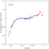 |
Fig. 1 TNG spectrum of asteroid (106) Dione (blue and red curves display the original blue and red spectra before merging), with the corresponding Gaia-like synthetic spectrum obtained by converting the TNG spectrum into a discretised signal mimicking what is expected from Gaia superposed (black points), as explained in Sect. 3. |
2.1 Obtained spectra
The observing conditions were variable during our different runs in terms of seeing, and on the night of October 31 2010, a fraction of the observing time was lost due to high humidity. In the November 2010 run, and, less frequently, also during the October 2010 run, the red part of the spectrum was often found to be quite noisy, and obliged us to discard parts of the long-wavelength end of the obtained reflectance spectra. Conversely, the blue part of the spectrum was always found to be more stable. The biggest problems we encountered were during our first observing run in October 2008 (see Sect. 2.2).
The full set of accepted reflectance spectra obtained in the two observing runs in 2010 is shown in Figs. A.1–A.6, in which the displayed spectra were smoothed by means of a running-box technique, generally using a box size of 50 data points. We note that in these figures we show the blue and red spectra as they were before merging, since the latter was done at the stage of spectra discretisation (see Sect. 3).
The reason we applied a running-box procedure to display the spectra was to smooth out many spurious spikes normally present in the raw data. The imperfect elimination of possible spikes at the two ends of the spectrum, which is a known property of the running-box technique, is not a real problem for our purposes, because any discretisation of the future Gaia spectra to smaller arrays of data points have similarly higher uncertainties at the ends of the considered spectral interval, corresponding to wavelengths where the detectors’ performance is sub-optimal.
In plots shown in Figs. A.1–A.6, the long-wavelength end of the blue spectra is systematically removed at wavelengths >0.77 μm, where the SNR becomes unacceptably low. In some cases, we also removed a portion of the lower- and upper-wavelength ends of the red part, whenever the data were judged to be exceedingly noisy based on a purely visual inspection. A very special case is that of asteroid (3997) Taga. This was a faint (V around 18) object when we observed it at high zenith distance, at the beginning of the night of November 10 2010. As a result, the obtained spectrum is, as expected, anomalous and certainly affected by large errors (specially in the red end), which make it absolutely unsuited for any scientific analysis. As discussed in Sect. 4.1, however, we purposely did not discard this spectrum, and we did not trim its red end, because we wanted to use it to test the behaviour of the software of taxonomic classification when dealing with a clearly abnormal case. The final spectra in digital form, corresponding to the figures shown in the appendix, will be made public on the web in a public repository (to be decided).
In general, the merging of the blue and red parts of the spectra was satisfactory. Some problems due to evident differences in spectral slope (the increase or decrease of reflectance going from blue to red) were found only in the cases of asteroids (1534) Nasi, showing a probably spurious reddening of the blue spectrum, and (14112) 1998 QZ25. In the case of (6815) Mutchler, the red part of the spectrum exhibits a progressive decrease that is probably not real, which was likely due to observing problems. Needless to say, in the case of asteroid (3997) Taga, the high-end of the red part of the spectrum makes no sense, but we kept it for the reasons explained above. We also note that two objects, (6698) Malhotra and (13100) 1993 FB10, were observed twice independently in the two observing runs in 2010 (the second run being executed a couple of weeks after the first one). In both cases, the two obtained spectra exhibited good mutual agreement (apart from some difference in the red region of the spectrum of (13100)).
In our figures, whenever possible we also plot an SMASS reflectance spectrum (Bus & Binzel 2002a) for each object. The agreement with our TNG spectra is generally satisfactory. The most notable exceptions are the cases of the bright S-class asteroid (39) Laetitia, and of the A-class asteroid (246) Asporina, both shown in Fig. A.1, for which we find steeper spectral slopes, specially in the case of Asporina. Since both asteroids were observed at fairly high phase angles, 19° and 22.3°, respectively, it is possible that we are seeing here, at least in part, some noticeable effect of spectral reddening at comparatively large phase angles. The SMASS spectrum of (39) Laetitia was obtained at a phase angle of 8.2°, while in the case of (246) Asporina, there are two published spectra, one obtained by Lazzaro et al. (2004) at a phase angle of 7.8°, and an SMASS spectrum consisting of an averaging of two observations, made at phase angles of 19.6° and 8°, respectively (Bus & Binzel 2002a). These two spectra show a nice mutual agreement and are clearly not as steep as the one obtained by us and shown in Fig. A.1.
The red part of the spectra of asteroids (742) Edisona (see Fig. A.2) and (7081) Ludibunda (see Fig. A.5) were also found to be significantly steeper, and therefore in fairly poor agreement with available SMASS spectra. In this case, however, the phase angles of our TNG observations of these two objects (listed in Table 2) are smaller than those of SMASS, namely 16.1° for (742), 25.9° for (7081), according to Bus & Binzel (2002a). Both objects are examples of targets that we observed at small phase angles, and were included in our target list only to cover unusual taxonomic classes (the SMASS K-class in both cases, see later). Therefore, the difference with the SMASS spectra could be due to reasons not related to the phase angle, possibly including differences in the solar analogues used and/or the applied air-mass corrections.
In the case of (1534) Nasi, already mentioned above and observed at TNG at a phase angle of 25.7°, the red and flat region of our spectrum is in very good agreement with an existing SMASS spectrum, observed at a phase angle of 15.7° by Bus & Binzel (2002a). The blue region, however, looks very different. Again, the reasons of this discrepancy can be due to a variety of possible reasons, although we tend to believe that our TNG spectrum for this objects might have an exceedingly steep slope in the blue region that is probably not real.
A full list of our targets, including information about the phase angle at each epoch of observation and the Tholen (1984) and Bus & Binzel (2002b) taxonomic classification (hereinafter Tholen and SMASS taxonomies, respectively) is given in Table 23.
We note that, in addition to objects known to belong to a large variety of taxonomic classes, we also obtained reflectance spectra for some relatively faint objects for which there was no previous taxonomic classification. We did this purposely, in order to include in our data set some faint and small bodies, which had never been observed spectroscopically before. We also note that we observed only main-belt asteroids, with the notable exceptions of the two large Jupiter Trojan asteroids (588) Achilles and (624) Hektor, both belonging to the D class, most of which are found among Jupiter Trojan asteroids. Finally, we mention that, in some cases, due to the need to include objects belonging to the largest possible variety of taxonomic classes in our data set, we also included some observations of objects seen at phase angles smaller than the typical Gaia values. In the case of the two Jupiter Trojans (588) and (624), phase angles lower than 10° are due to the heliocentric distance of the objects, and are thus also true for Gaia observations. For reasons explained below, not all the objects listed in Table 2 were used in the next steps of our analysis. In particular, we did not make use of the spectra of objects that in the above Table are not identified as “cloned”.
2.2 Some problems
It is known that asteroid reflectance spectra observed at different epochs and using different detectors often exhibit relevant differences, mainly for what concerns the slope of the spectrum from blue to red, and the depth of the main absorption bands around the wavelength of 1 μm. Sometimes such differences are considered to be a consequence of surface heterogeneity, but this interpretation is often questionable. This issue was the subject of an extensive analysis of a variety of reflectance spectra obtained in different epochs for the moderately large and bright main-belt asteroid (354) Eleonora (Gaffey et al. 2015). These authors noted that the CCD spectra at visible wavelengths of this asteroid “show apparently irreconcilable differences”, whereas the situation appears to be better in the near-IR.
Although we are probably still far from obtaining a complete understanding of the origin of the problem, there are good reasons to believe that differences among spectra of the same object obtained by different observers at different epochs are the effect of a variety of mechanisms playing a role at the same time, including varying observing conditions, differences in the adopted solar analogue stars, imperfect telescope tracking during the exposure, tiny wavelength calibration errors, and, sometimes, questionable observing practices, normally due to the need of many observers (including possibly ourselves!) to maximise the number of obtained spectra at the cost of data quality (for instance, by observing when sky conditions are unfavourable).
In particular, the choice of the solar analogue star used to divide the asteroid spectrum is a longstanding issue (see, again, Gaffey et al. 2015). We know that not all the solar analogue stars present in the catalogues are really identical. This effect is particularly important in the blue part of the spectrum, where solar analogue stars often exhibit non-negligible differences with respect to one another and to the solar spectrum (Ramirez et al. 2012). The two stars 16 Cyg B and Hyades 64, the latter having been used in all our observations, are often considered by many asteroid observers to be among the best possible choices, because they are bright and used in many observing programmes.
In our 2008 observing run, we observed and used both 16 Cyg B and Hyades 64 to produce the reflectance spectra of all the observed asteroids. However, in reducing the data, we found that the resulting reflectance spectra computed by using the two above-mentioned stars observed in the same night turned out to be quite different in many cases. A representative example is shown in Fig. 2. The observed behaviour in this particular case could be due to saturation of one of the two solar analogue stars at some wavelengths. Whenever possible, however, we compared the two resulting spectra of each asteroid in our sample with spectra of the same object available in the SMASS survey. We found that in some cases, like that of (32) Pomona shown in Fig. 2, the reflectance spectrum obtained at TNG using 16 Cyg B as a solar analogue star was in good agreement with a published SMASS spectrum. In other cases, however, a good agreement was found between the SMASS spectrum and the one obtained at TNG using the solar analogue star 64 Hyades. Even more important, for 12 observed asteroids out of 30 present in the SMASS catalogue (Bus & Binzel 2002a), the obtained TNG spectra turned out to be in strong disagreement with, (or in some cases completely different from) the corresponding SMASS spectrum, independent of the choice of the solar analogue star.
As a consequence of this anomalous behaviour, which we were not able to explain, we decided to exclude all the data obtained in the 2008 run from our analysis. Fortunately, we were lucky enough to obtain a sufficient number of asteroid spectra during the two 2010 runs, which were not affected by the problems described above.
We end this discussion by noting that, based on our experience, it seems that the best practice to minimise the role played by solar analogue stars in the measurement of asteroid reflectance spectra would be probably to use, as Farnham et al. (2000) and Tedesco et al. (1982) did, averaged spectra of several of the best solar analogue stars, to be observed each night. We cannot do this in the present analysis because, as shown in Table 1, in general each night we observed only two solar analogue stars, and not the same ones every night. We believe that making averages of only two different stars per night, mostly observed at different air masses, would not improve the robustness of our results.
Asteroids observed in the observing campaign described in this paper.
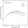 |
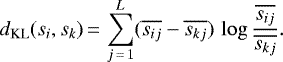
Fig. 2 Reflectance spectrum of asteroid (32) Pomona obtained during our 2008 observing run. The resulting reflectance spectra are significantly different, depending upon the adopted solar analogue star. One of the two spectra (corresponding to solar analogue 2, blue+red curves) is in very reasonable agreement with the SMASS spectrum of this asteroid, whereas the use of solar analogue 1 produces a quite different reflectance spectrum at all wavelengths. SA1 and SA2 correspond to solar analogue stars Hyades 64 and 61 Cyg B, respectively. |
3 Conversion of TNG spectra to expected Gaia signals
As explained in the recent paper by the Gaia Collaboration (2016) and, earlier, by Delbò et al. (2012), the light incident on each of the Blue Photometer (BP) and the Red Photometer (RP) detectors on the Gaia focal plane is dispersed along the Gaia scanning direction and spread over about 45 pixels. The along-scan window size around the observed object, namely the region of the CCD, which is actually read and transmitted to the ground, is chosen to be 60 pixels in length for each of the two detectors. The spectral dispersion varies in BP from 0.003 to 0.027 μm pixel−1 over the wavelength range 0.330–0.680 μm and in RP from 0.007 to 0.015 μm pixel−1 over the wavelength range 0.640–1.050 μm, resulting in a resolving power that varies between 70 and 20 for BP and between 90 and 70 for RP, as shown in Fig. 2 of Delbò et al. (2012). As a consequence, the line-spread function conveys 76% of the incident energy into 1.3 pixels at 0.330 μm and into 1.9 pixels at0.680 μm along the BP spectrum. Along the red spectrum, the above numbers become 3.5 pixels at 0.640 μm and 4.1 pixels at1.050 μm. For all but the brightest objects, namely those brighter than 11.5 mag in the Gaia G band (van Leeuwen et al. 2018), BP and RP spectra are binned on-chip in the across-scan direction over 12 pixels. Correspondingly, a Gaia spectrum consists of a 1D array of 60 + 60 pixels (60 for BP and 60 for RP). Further binning of the pixels where the signal is recorded produces a discretisation of the Gaia spectrum to a smaller array of data points, of which the final number will be decided based on optimisation of the data reduction pipeline.
The purpose of our analysis was to use our TNG spectra as a basis of prototypes aimed at mimicking the variety of possible cases expected for Gaia asteroid observations. As a first step, we performed a discretisation of our reflectance spectra, in order to bring the DOLORES-TNG spectroscopic observations that have a higher spectral resolution to the typical resolution of the Gaia BP-RP spectra. Each spectrum was converted into a set of 30 discrete values of spectral reflectance, from blue to red, normalised at 0.55 μm. First, we determined the centre and widths (Δλ) of bins in wavelengths that would correspond in the range 0.4–0.95 μm to the resolution of the combined BP and RP reflectance spectra. For this, we used the λ-dependent Δλ values as given in Fig. 2 of Delbò et al. (2012). We started with a bin centred at a wavelength of 0.4 μm and we proceeded with adjacent bins of wavelength-dependent width until we reached the wavelength of 0.95 μm. The longer wavelength bin is centred at 0.94 μm. Next, within each wavelength bin we determined the average  and the standard deviation of the TNG reflectance values σR. For the uncertainty of
  , we take
  , where N is the number of data points in the bin. In the region where the wavelength bins receive the contributions from both the blue and the red arm of the spectrometer (e.g. between ≈0.65 and 0.75 μm), we considered both contributions to calculate the mean and the standard deviation. An example of discretisation of one of our TNG spectra, in particular the one of the Cgh-class asteroid (106) Dione is shown in Fig. 1.
We note that, in our discretisation procedure, we did not consider wavelengths shorter than 0.4 μm, while the extreme red end was chosen at about 0.95 μm. Outside thiswavelength interval, the quantum efficiency of the CCD detector used at TNG starts to drop significantly. The above limits should be fully comparable with those characterising the spectral region where Gaia measurements are expected to have satisfactory SNR. We note that, in the blue, a wavelength limit of 0.4 μm is usually well below the lower limit of the wavelength interval covered by ground-based observations, except possibly for a few very bright objects. In this sense, our TNG spectra meet our requirements to reasonably approximate the signals expected forGaia. We believe therefore that our analysis described in the following sections represents a realistic model of what we expect to be the treatment of the Gaia data that will be used to derive a Gaia-based asteroid taxonomy.
We note that we did not apply our discretisation procedure to the total set of our TNG spectra, but only to a smaller sub-sample of 33 objects that we chose as suitable taxonomic end members of the whole population. These objects were subsequently used as prototypes to generate the large set of spectral clones described in the following section, used as input to our taxonomic classification algorithm. Table 2 specifies which asteroids we used for this purpose. We note that for some of them, our reflectance spectra are not of the highest quality. We included them in our analysis because they may well be representative of situations that may beencountered in the case of future Gaia measurements of faint asteroids close to the magnitude limit (G = 20.7) of the mission. We also note, however, that the uncertainties in the reflectance spectra obtained from measurements of single transits on the Gaia focal plane will decrease by adding spectra of the same objects taken at different transits (Delbò et al. 2012), assuming that the spectra do not change with time. Of course, even so, the SNR is lower for faint objects close to the Gaia magnitude cut-off even for the most favourable Gaia transits.
We discarded sixteen asteroids from our original data set from our analysis, because they were not relevant for our test case. They were chosen according to at least one of the following criteria: (1) objects having low-quality spectra, being exceedingly noisy and/or showing a bad merging of the blue and red regions, according to a purely visual inspection of the data; (2) objects showing flat and featureless spectra corresponding to the populous C-complex, both already classified and previously unknown4; and (3) objects observed at phase angles smaller than about 10°.
As previously mentioned, we included the asteroid (3997) Taga (not previously classified) on our list only because its spectrum (shown in Fig. B.4) is totally anomalous, having been obtained in very special conditions, at a very high zenithal distance. The purpose was to check that such anomalous spectral morphology would lead, as expected, to classifying this object and its clones (see below) as a separate taxonomic class, in order to verify the behaviour of our adopted taxonomic classification algorithm. For the same reason, we also made use of the spectrum of (1662) Hoffmann (shown in Fig. B.3), classified as a member of the SMASS Sr class. Also in this case, the red region of our TNG spectrum is peculiar, though not as extremely as (3997).
4 Cloning of observed spectra
4.1 The cloning algorithm
A data set of only 33 asteroid spectra is certainly not sufficient for the purpose of simulating a taxonomic classification based on Gaia observations of 105 asteroid spectra. However, our tiny sample includes a large variety of objects, which can be considered as representative end members of the vast majority of the asteroid population, according to current knowledge. Apart from a few exceptions, our spectra have also been obtained in observing circumstances corresponding to those of Gaia observations, namely at phase angles larger than 10°. The idea therefore is that each and every spectrum of our selected sample can be used as a prototype of its class. As a consequence, each spectrum can be cloned many times to build a large sample of synthetic spectra, which would be sufficient to serve as input to a taxonomic classification algorithm. Within each asteroid taxonomic class, the reflectance spectra of the objects are similar, but not identical. The differences can be far from negligible in many cases, primarily for members of the large S and C complexes and their respective sub-classes. Even under the unrealistic assumption that the spectra of all members of a given taxonomic class were identical, different observations of the same object at different epochs could not be expected to produce identical reflectance spectra, due to random fluctuations of the signal when an object is observed at different epochs, or as a consequence of differences in the apparent motion across the Gaia focal plane at different transits.
It is therefore necessary to create a large number of spectral clones for each object of our adopted sample, but these clones cannot be identical to their prototypes to mimic a realistic spectroscopic survey.
We developed an algorithm to produce spectral clones using a very simple numerical approach. The first step of the cloning procedure, once the spectrum to be cloned is chosen, is the random choice of one of 28 wavelength components of its digitised spectrum, λi. The number 28 takes into account the fact that we do not want to modify either the first or the 30th wavelength component, in order to avoid simply “pulling” one of the ends of the spectrum up or down. A random change, taken from a Gaussian distribution with zero mean and σ = 0.05 in normalised reflectance, is assigned to the corresponding spectral reflectance SR(λi). This means that in morethan 99% of the cases, the spectral deformation is smaller than 0.15 in absolute value. In those cases where the total amplitude of the spectrum is smaller than 0.2 in normalised reflectance, we assign a value of σ equal to 0.2 times the total spectral amplitude. The reason being that we do not want to apply exceedingly large perturbations to spectra that are intrinsically flat, producing clones that completely alter the spectral trend of their parents.
Once the spectrum is modified at the randomly chosen wavelength λi, the procedure continues by assigning spectral reflectance changes with the same sign of that of the point at λi to the remaining surrounding wavelengths, but these changes are chosen in such a way as to gradually decrease to zero, on both sides of λi, for increasing differences in wavelength. A check is done to take into account situations in which the non-altered reflectance could be quickly increasing or decreasing around λi, in order to avoid the possibility of our artificial modification of reflectance at wavelengths λj ≠ λi producing an unreasonable increase in already steep spectral slopes.
Based on the developed procedure, the reflectance values at wavelengths far from the randomly chosen λi always tend to remain very limited if not totally unchanged.
After that, a further, minor shift is assigned at all wavelengths, corresponding to a random Gaussian noise with zero mean and σ = 0.015 in normalised reflectance, independent of the main spectral variation applied in the first step. The amplitude of this further noise is chosen to be very small, taking into account that the single digitised components of our spectra consist of values of the flux averaged over non-negligible intervals of wavelengths.
At the end of the procedure described above, a final and constant spectral shift is assigned to each reflectance component, if needed, to ensure that SR(λ = 0.55 μm) is always equal to 1, to keep the standard normalisation of the spectrum.
To summarise, a clone is produced by (1) gently “pulling up or down” one component of the spectrum; (2) propagating an increasingly smaller deformation to the neighbouring wavelengths; and (3) applying a further, minor noise at all wavelengths, to simulate random fluctuations. In this way, it is extremely quick and simple to produce very large numbers of spectral clones, starting from our set of spectral prototypes. As an example, we show in Fig. 3 the total envelope of the 71 randomly generated clones of our TNG spectrum of asteroid (1929) Kollaa.
4.2 Modeling a realistic distribution of asteroid spectra
Using the cloning algorithm described above, we generated a population of 10 000 synthetic asteroid reflectance spectra, to be used to test the Gaia algorithm of taxonomic classification.
A very important fact concerning asteroid taxonomy is that the currently identified taxonomic classes are not equally populated. It is known that two major spectral complexes, S and C, are most abundant in the inner and in the outer regions of the belt, respectively. A large number of smaller classes are also present, their contribution to the total asteroid inventory being much more limited with respect to S and C.
We took all this into account when we generated our artificial population of 10 000 spectra. This means that in our procedure of cloning ofour selected TNG spectra, we did not simply choose a spectrum to be cloned randomly at each step from those in our TNG sample. In order to produce a more realistic population, we assigned to each observed spectrum a different probability to be chosenat each step by the cloning procedure. In so doing, we based our criteria on the results of the SMASS survey, as well as on an analysis of the PhD thesis of S.J. Bus, in which the results of the SMASS survey were critically assessed and extensively discussed (Bus 1999).
We considered five major taxonomic assemblages:
-
Assemblage I including SMASS classes C, Ch, B, Cb, Cg, Cgh, assumed to account for 45% of the whole bias-corrected asteroid population.
-
Assemblage II including SMASS classes S, Sl, Sk, K, Sq, Sr, assumed to account for 30% of the whole bias-corrected population.
-
Assemblage III including SMASS classes X, Xe, Xk, Xc, assumed to account for 18% of the whole bias-corrected population.
-
Assemblage IV including SMASS classes L, V, Ld, D, T, assumed to account for 5% of the whole bias-corrected population.
-
Assemblage V including SMASS classes A, R, Sr, Q, assumed to account for 2% of the whole bias-corrected population.
We note that what we call here “taxonomic assemblage” has little to do with the surface compositions of the objects. They have been defined with the relative abundances of asteroids belonging to different taxonomic classes in mind. Of course, assemblages I to III correspond to well-known taxonomic complexes (C, S, X), but assemblages IV and V are purely arbitrary. We then used the above scheme to assign each of our 33 selected TNG spectra to one of the assemblages defined above. In some cases where asteroids lack a previous SMASS classification, we assigned them to one of the assemblages based on a visual inspection of the spectrum. Having defined the spectral assemblages and the corresponding members of each of them in our selected TNG spectra, we launched the spectral cloning procedure in the following way: at each step, we randomly selected the assemblage to which the new clone had to belong by considering a probability corresponding to the different abundances of objects belonging to the different assemblages. Having selected the assemblage, we then randomly chose, from the TNG spectra included in our sample and belonging to the selected assemblage, the one to be cloned at that given step.
It is clear that the procedure described above is not exempt from possible criticisms. On one hand, the grouping of the different classes among the five main assemblages could have been done in a number of different ways. Moreover, the details of the relative abundances assigned to the five major assemblages can also be improved, and they are not based on the most recent analyses of this subject. For instance, we could have used the results of the more recent work by DeMeo & Carry (2013), based on measurements in five bands of the Sloan Digital Sky Survey (Ivezić et al. 2001, 2002), but we preferred to adopt the older SMASS results because they are based on spectra more like those obtained in our observing campaign. Possibly even more important, the choice of assigning an identical probability to pick up at each step one of the different classes belonging to the selected assemblage can also be questionable. We are aware of these possible criticisms, but on the other hand, we stress that in our present analysis we are only interested in producing a reasonable population of synthetic asteroid spectra, to serve as input to the taxonomic classification algorithm described in the next section and for the sole purpose of testing its performances. For this reason, we do not think that we should spend much more time and effort in order to produce a possibly more realistic synthetic population, but in any case not dramatically different with respect to the one we generated by means of the simple algorithms described in this paper. In the last column of Table 2, we specify, for each spectrum selected for cloning, the corresponding assemblage to which it has been assigned.
Even before analyzing our results in Sect. 6, we can make some predictions, based on what we know to be some well-established problems in defining a taxonomic classification based on spectroscopic or spectro-photometric data covering visual wavelengths only. In particular, the well-known degeneracy of the E, M, and P classes, firstrecognised by Gradie & Tedesco (1982), which later became the SMASS X complex, and which they noted cannot be avoided in the absence of ancillary information such as albedos or near-IR data, has most recently been confirmed by the results of DeMeo et al. (2009; hereinafter, DeMeo taxonomy).
We have already mentioned that the major characteristics of the future Gaia taxonomy will be the inclusion of spectral reflectance data down to 0.4 μm, if not at even shorter wavelengths for the brightest objects, and its basis on spectra obtained at phase angles larger than 10°.
As far as the spectral properties in blue are concerned, we must admit that the set of objects we observed, and their corresponding clones, do not sufficienty cover certain taxonomic classes for which it would be of the highest interest to see whether they can be identified based on the behavior at the shortest wavelengths. An important task would be to investigate the possibility of using Gaia spectra to distinguish, among asteroids belonging to the SMASS and DeMeo B taxonomic class, those that would be more appropriately classified as F-class (see Sect. 1). The possibleidentification of the F class based on reflectance spectra limited to visible wavelengths including the blue region will be a matter of investigation when Gaia spectra are obtained and published, and it is largely beyond the purposes of the present analysis. We note, however, that we included in our list of selected TNG spectra to be cloned at least one object exhibiting a very flat trend (though not formally belonging to the F class), namely (6661) Ikemura, an asteroid for which no taxonomic classification is available in the literature.
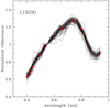 |
Fig. 3 TNG spectrum of asteroid (1929) Kollaa converted into Gaia format (red points), and surrounded by the envelope formed at each wavelength by its clones (71 in number), generated randomly using the technique described in the text. |
5 The classification algorithm
The asteroid taxonomy produced at the end of the Gaia mission will be based on Gaia spectroscopic data, only. Further refinements including input data coming from other data sources will be postponed to the immediate post-Gaia era. In this paper, we test the taxonomic classification algorithm designed for Gaia as it is (Galluccio et al. 2008). This means that we do not consider other dimensions of the physical parameter space, as could be done, for instance, by making use of additional albedo data coming from WISE thermal radiometry data, or from polarimetry.
We have used the large data set of synthetic asteroid reflect- ance spectra, obtained using the cloning procedure described in Sect. 4, to serve as input to the classification algorithm developed by some of us involved in the Gaia Data Analysis and Processing Consortium, for the purpose of using Gaia spectra of asteroids to obtain a new taxonomy of the asteroid population. This is the algorithm, described by Galluccio et al. (2008), that will be used to produce the final asteroid taxonomy included in the Gaia catalogue atthe end of the mission. It is an unsupervised algorithm, meaning that no a priori assumptions are made, and the spectral reflectance data are used for classification purposes without making use of of any ancillary information.
The algorithm is based on a method for partitioning a set S of N data points, with S ∈ℜL, where L in our case is the number of spectral bands (L = 30, corresponding to our discretisation of the spectra), into K non-overlapping clusters such that: (a) the inter-cluster variance is maximised and (b) the intra-cluster variance is minimised.
The first step is to introduce a metric to quantify the distances between the objects in the space of our spectroscopic data. In our application, we used the so-called Kullback-Leibler metric, defined as follows. Let si = si1, si2, …, siL be a vector representing a given spectrum (defined by its L discrete values of reflectance). At any given wavelength λj each spectrum can be associated to a positive, normalised quantity:
which can be interpreted as the probability distribution that a certain amount of information has been measured around the wavelength λj. The similarity between two probability density functions can then be measured by computing the so-called symmetrised Kulbach-Leibler divergence, which therefore becomes the metric dKL (si, sk) that we need to measure the distance between two spectra, si and sk:
 (1)
(1)
Once the metric has been defined, the distances between the different objects (spectra) of the given sample can be computed. We can therefore compute the total length of different possible “trees”, namely the total distance obtained by linking together all the spectra in all possible ways, computing the distance of each segment, but never using a given spectrum more than once. The clustering approach is based on the concept of the minimal spanning tree (MST), and data partitioning. In particular, the MST is the tree passing through each object of the set (which becomes a “vertex of the tree”) that has the minimal possible total length. Under the assumption that the distribution of the vertices of the tree is well approximated by a Poisson distribution, the MST is computed using the so-called Prim’s algorithm, as explained in Galluccio et al. (2008). The idea is that a function (referred to as Prim’s trajectory) retrieves the distance of the connected vertices of the tree (here asteroid spectra) at each iteration. Then an automatically computed threshold is applied to this function. The sets of spectra below the threshold are considered as clusters. We use a popular clustering algorithm, K-means, to partition the resulting data clusters and obtain the final classification. We note in this respect that the value of K, corresponding to the number of resulting clusters, is usually decided a priori when using the K-means algorithm, but here K is not a parameter chosen subjectively after a visual inspection of the data, but it is “objectively” determined by the previous steps of the algorithm, as pointed out by Galluccio et al. (2008).
Number of clones generated for each parent spectrum, and number of them found to be members of each of the twelve taxonomic classes resulting from the classification exercise.
6 Results
The results of the taxonomic classification using the methods described in Sect. 5 are summarised in Table 3, which lists for each of the 33 selected TNG spectra (“parent spectra”) the number of clones found to belong to each of the classes identified by the classification algorithm. Twelve distinct classes were found. In general, the vast majority of the clones of the same parent spectrum tend to be classified as members of only one of the twelve identified classes. In some cases, however, significant fractions of clones of the same parent are classified as members of a few other classes. This is not surprising, because our selected parent spectra include several objects belonging to sub-classes of some wider taxonomic complex, (the S, or C, or X complex), and these sub-classes exhibit often only small differences in their spectra. For this reason, even small spectral modifications like those determined by our cloning procedure can sometimes be sufficient to move a spectrum from one class to another.
In several cases, all the clones of a given parent spectrum are found to be members of only one taxonomic class. This happens, as expected, in the case of the clones of the spectrum of (3997) Taga, already mentioned in previous sections. This is the positive result of a test aimed at confirming that an anomalous spectrum would produce clones that are all well separated from the rest of the population and define an exclusive class (named Class 11 in Table 3). Another interesting case is that of (1662) Hoffmann. The parent asteroid is classified as Sr by both the SMASS and DeMeo taxonomies. Its TNG spectrum, shown in Fig. A.3, is noisy at long wavelengths, and in generating its clones after discretisation, we also included a couple of points in the red region that are discrepant with respect to their neighbours. All 320 generated clones strictly follow the trend of the parent spectrum, as shown in Fig. B.8, therefore producing a distinct class, indicated as Class 07 in Table 3. The comparatively high number of clones of this object is a consequence of the fact that it belongs to the abundant S complex.
More interesting are the cases of “clean” parent spectra of asteroids belonging to rare taxonomic classes: for example, in the cases of (246) Asporina, (1929) Kollaa, and (269) Justitia. The spectra of these asteroids, together with the envelopes of their clones, are shown in Fig. B.8. (246) Asporina is a member of the rare A class according to the Tholen, SMASS and DeMeo classifications. As shown in Table 3, all 43 of its generated clones belong to a unique class, named Class 12 in our analysis. Figure B.8 also shows that our cloning procedure described in Sect. 4 tends, as expected, to leave the spectral regions characterised by a very sharp and steep slope unaltered, whereas differences among the clones are much more evident in the regions where the parent spectrum is not so steep. We note that, among our selected parent spectra, those of asteroids (246), (1126), and (2715) are all classified as members of the A-class in the SMASS taxonomy. However, if one looks at the DeMeo taxonomy, which is based on spectra that also include the near-IR wavelength region, only (246) is classified as A, whereas both (1126) and (2715) are classified as Sw. Interestingly enough, our classification algorithm also assigns (1146) and (2715) to different classes with respect to (246).
The asteroid (1929) Kollaa is the only one in our selected sample belonging to the V taxonomic class, according to both SMASS and DeMeo. Another of our selected parent spectra, (1904) Massevitch, is classified as R by SMASS, whereas it is another V class according to the DeMeo taxonomy. The V class, believed to include mostly fragments of the large asteroid (4) Vesta, is characterised, at visible wavelengths, by a very strong and wide absorption band around 1 μm. The reflectance spectrum of (1929), together with its 71 generated clones, is shown in Fig. B.8. All of them are found by our classification algorithm to define a separate class, named Class 10. Interestingly enough, the spectrum of (1904), shown in Fig. A.3 shows a much less pronounced absorption band in the red, and its clones are found in a separate class (Class 09).
Our observed TNG spectrum of (269) Justitia is very reddish, and its 80 clones form a distinct class (named Class 06 in Table 3). This asteroid has been classified as Ld in the SMASS taxonomy, while it is classified as D-class in the DeMeo taxonomy. We note that two other parent spectra in our list, those of (624) Hektor and (588) Achilles were classified as members of the D class in the Tholen taxonomy. Being Jupiter Trojans, neither of them is included in the SMASS or the DeMeo taxonomy, since both were covering main-belt asteroids only. More precisely, (588) was classified as DU by Tholen, implying a more uncertain classification. All published taxonomies concur on the fact that the D class includes very reddish spectra, which are common among Jupiter Trojans. As shown in Table 3, however, the clones of (624) and (588) do not merge with those of (269) Justitia. A comparison between the TNG spectra of the three parent objects, shown in Fig. 4, shows that our observed spectral slope of (269) is significantly steeper than those of (624) and (588), which are very similar to each other. This fact explains the different classification of (269) in a separate class, and shows that our code of taxonomic classification is sensitive to the overall spectral slope. We are led to conclude that the D DeMeo classification of (269) Justitia might be questionable. We note also that the SMASS classification as Ld corresponds also to a very red object. Of course, the very steep spectral slope of our TNG spectrum for this asteroid needs some confirmation. In this respect,we note that (269) is one of the few asteroids in our selected sample that was observed at a small phase angle, around 5°, and for this reason no phase reddening effect can explain the steep spectral slope that we found.
Table 3 shows that among the 12 classes identified by our classification algorithm, two are dominant, since they includevery large numbers of cloned spectra. These classes are indicated as Class 01 and Class 02. In some cases, all the generated clones of some of our selected parent spectra belong either to Class 01 or Class 02, like in the case of the clones of asteroid (261) Prymno, all belonging to Class 01, or asteroid 175 Andromache, whose clones are all classified in Class 02. There are, however, several cases in which, among the clones of a given parent spectrum, the vast majority belong to either Class 01 or Class 02, but a small fraction of them belong to the other class. Two examples are given by the clones of (106) Dione and (8424) Toshitsumita.
Because the total number of generated clones that are classified as members of either Class 01 or Class 02 is so high, for the sake of clarity in Figs. 5 and 6 we only plot together the TNG spectra of the parent asteroids whose clones contribute to Class 01 and Class 02, respectively. In these figures, we use larger symbols to indicate the parent spectra of clones belonging mainly to one of the two classes, and we use the same colour, cyan and blue respectively, to indicate Class 01 and Class 02, respectively.
By looking at Figs. 5 and 6, we can see that the differences between the general trends of the parent spectra contributing to these two classes are not so sharp in some cases. In general, Class 02 is more compact, and exhibitsa flatter trend from blue to red, whereas Class 01 is characterised by a generally reddish trend, but with a noticeable range of variation in the red region. It also displays a more pronounced fall in the blue region, similar to, but stronger than Class 02, which also tends to display a decrease in reflectance towards the blue end. The difference between the blue and red reflectance seems to be, therefore, the decisive factor in determining the classification as either Class 01 or Class 02, the former exhibiting a sharper increase of reflectance moving from blue to red.
Interestingly, if we look at the Tholen, SMASS, and DeMeo taxonomic classification of the parent spectra producing clones belonging to Class 01 and Class 02 in Table 3, we find some interesting features. Class 01 includes the clones ofasteroids belonging to a large variety of classes: among its major contributors, we find asteroid (96) Aegle, belonging to the T class according to all the three above-mentioned classifications. Asteroid (106) Dione belongs to the G Tholen class and to the Cgh SMASS and DeMeo classes. Asteroid (261) Prymno is a Tholen B class, and a SMASS X class. Asteroid (1214) Richilde is a SMASS Xk class. Asteroid(1471) Tornio is a SMASS T and DeMeo D class. Asteroid (3451) Mentor is a SMASS X class.
Class 02 is much more homogeneous, including spectra that are classified as C, Cg, or Ch according to the above-mentioned classifications. It also includes objects that are not classified, but exhibit a flat TNG spectrum, like in the cases of (5924) Teruo and (8424) Toshitsumita, as shown in Figs. A.4 and A.5. We are led to conclude that our Class 02 generally corresponds to the C complex and its sub-classes, but it is interesting to see that some C sub-classes such as Tholen G and SMASS and DeMeo Cgh are found in Class 01. Class 01 turns out to be fairly heterogeneous, merging together spectra belonging to the X complex, which is known to include objects of different albedo.
Since the main characteristic of our Class 01 seems to be a moderately reddish trend, we cannot rule out the possibility that objects belonging to some C sub-classes, in particular the SMASS Cgh class, when observed at comparatively large phase angles, as in the case of our TNG observations, might display some noticeable phase reddening, a hypothesis that needs new data to be confirmed. We also note that the Tholen B classification of (261) Prymno appears quite surprising, because most B class objects exhibit blueish reflectance spectra, whereas the SMASS classification as X looks more credible.
The case of the spectral clones of asteroid (6661) Ikemura is also interesting. We included this object in the set of our selected parent spectra because, in spite of it being an unclassified object, (6661) exhibits a TNG spectrum that is very flat in the whole interval of covered wavelengths, which is a typical behaviour of the old F class. A slight blueish trend could also be diagnostic of the SMASS B class. The results have shown that all 730 of the clones of (6661) are found in one and only one resulting class, namely Class 03, togetherwith a few other clones of a couple of other parents that are major contributors of clones found in Class 02. Figure 7 shows the spectra of the clones of (6661) Ikemura as continuous lines, while the few additional clones coming from the two parent bodies (5924) and (919) are displayed as points corresponding to their discretised spectra plotted above the envelope of the (6661) clone spectra. These additional clones also share the property of displaying a generally flat trend and no or very little decrease in reflectance at the shortest wavelengths.
While we set aside the analysis of our Class 04 (see below) for a moment, we now make some comments about Class 05, as listed in Table 3 and shown in Fig. 8. This class is quite heterogeneous in composition, as it is formed by clones of parent spectra belonging to different taxonomic classes according to current classifications. They include (179) Klytaemnestra (Tholen S, SMASS Sk), (588) Achilles and (624) Hektor (both Tholen D-class), (742) Edisona (Tholen S, SMASS and DeMeo K), (2354) Lavrov (SMASS and DeMeo L), (2715) Mielikki (SMASS A, DeMeo Sw), and (7081) Ludibunda (SMASS K), plus a few other clones of other parent spectra. The envelope of the spectra of the clones producing Class 05, shown in Fig. 8, exhibits a steep spectral slope from blue to red, steeper than in the case of Class 01 previously described. At the longest wavelengths, there is an apparent dichotomy, with some spectra, including those of the clones of the two Jupiter Trojans, (588) and (624), and of the K-class asteroid (7081), which show a monotonic increase of reflectance up to the red end of our TNG spectra, coexisting with a majority of spectra by the other clones, whose parents mostly belong to the K class, and the Sk and Sw sub-classes of the S complex, which show a very mild absorption band centred around 0.9 nm. Interestingly, the clones of Barbarian asteroid (2354) Lavrov display the same behaviour. Barbarians are asteroids exhibiting peculiar polarimetric and spectroscopic properties (see Devogèle et al. 2018b, and references therein). In summary, our Class 05 merges spectra that are monotonically and steeply red, and spectra, which, after a steep increase from blue to red, display a very mild and shallow absorption band, in the region expected for members of the large S complex. We are led to conclude that our taxonomy classification algorithm does not find a clear separation between the two above-mentioned spectral morphologies. This fact has to be taken into account in view of possible improvements and fine-tuning the algorithm, to be done before processing real Gaia data in the near future.
The cases of classes 04, 08, and 09 are shown in Figs. 9–11, respectively. It is useful to compare these figures, in particular with regard to their mutual differences. All three kinds of spectral behaviour generally correspond to what is displayed by asteroids belonging to the S complex, and all the parent spectra of the clones belonging to these three classes belong, where available, to the Tholen S class. The distinction between Classes 04, 08, and 09 seems to be mostly due to the depth of the absorption band around 0.9 nm, which is found to increase from Class 04 to Class 08 to Class 09. Some possible dichotomy in the behaviour of Class 05 members, with some of them displaying a deeper absorption band at the longest wavelengths, is also visible. There are also some differences in the spectral slope at shorter wavelengths, with Class 04 being slightly steeper than Class 08, which in turn is slightly steeper than Class 09. We note that, in terms of known taxonomic classification of the parent spectra, the SMASS Sq class tends to be represented in both Classes 08 and 09, with some exchange of clones between the two classes, further proof that the separation between the two is fairly fuzzy. The DeMeo class Sw tends to be dominant in Class 04.
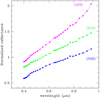 |
Fig. 4 TNG normalised reflectance spectra of asteroids (624) Hektor, (588) Achilles, and (269) Justitia. To avoid overlapping, the spectra of (588) and (269) have been shifted by ± 0.2 with respectto the spectrum of (624). |
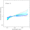 |
Fig. 5 TNG normalised reflectance spectra of the selected asteroids whose clones are found in the resulting Class 01. Parent spectra whose clones exclusively (or the vast majority) belong to Class 01 are plotted in cyan. Parent spectra of clones mostly contributing to Class 02 are plotted in blue. Parent spectra providing only very minor contributions to Class 01 are plotted with small symbols. The black colour refers to very small numbers of clones of parent bodies mostly contributingto classes other than Class 01 or Class 02. |
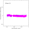 |
Fig. 7 Spectra of clones of the spectrum of (6661) Ikemura (magenta lines), with the discretised spectra of a few clones of parent spectra (919) and (5924) superimposed, which were also found to belong to Class 03 in our taxonomy exercise. |
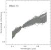 |
Fig. 8 Spectra of clones classified in Class 05. Continuous grey lines indicate clones of the (179), (588), (624), (742), (2354), (2715), and (7081) parent spectra, whose clones are totally or predominantly found to contribute to this class. Some additional discretised spectra of a few clones of parent spectra (1126), (5142), and (13100), which are also found to be classified as Class 05, are superimposed in different colours. |
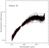 |
Fig. 9 Spectra of clones classified in Class 04. Continuous black lines indicate clones of the (39), (1126) and (219071) parent spectra, whose clones are totally or predominantly found to contribute to this class. Some additional discretised spectra of a few clones of parent spectra (2354), (2715), and (7081), also found to be classified as Class 04, are superimposed in red. |
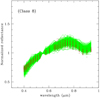 |
Fig. 10 Spectra of clones classified in Class 08. Continuous green lines indicate clones of the (82), (808), and (13100) parent spectra, whose clones are totally or predominantly found to contribute to this class. Several additional discretised spectra of clones of parent spectrum (5142) are superimposed in brown, as well as a few clones of parent spectra (179), (742), and (2715), also found to be classified as Class 08, are superimposed in grey. |
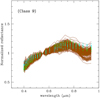 |
Fig. 11 Spectra of clones classified in Class 09. Continuous brown lines indicate clones of the (720), (1904), and (5142) parent spectra, whose clones are totally or predominantly found to contribute to this class. Some additional discretised spectra of clones of parent spectra (82) and (808) are superimposed in green, while a few clones of parent spectra (261) and (1214), also found to be classified as Class 09, are superimposed in cyan. |
7 Conclusions and future work
In the present paper, we used a small sample of asteroid spectra, obtained with the constraint of being fully representative of what we canexpect to be the catalogue of Gaia spectroscopic data for asteroids, to build a large set of artificial asteroid spectra, distributed according to currently known abundances of different taxonomic classes throughout the asteroid main belt, and in the Jupiter Trojan region. This large sample was used as the input to the algorithm for taxonomic classification developed to analyse Gaia asteroid data, because the main goal of our exercise was to conduct a preliminary test of the performance of this algorithm.
We are aware that many assumption we made in the present work, mostly concerning the generation of spectral clones, have been made for sake of simplicity rather than realism, and the results are certainly affected by these choices. As an example, the number of clones generated for any given parent spectrum has certainly some influence on the way the taxonomy algorithm identifies a variety of resulting classes and their mutual separations. It is reasonable, therefore, to think that the different numbers of clones generated for different parents are important in determining the resulting taxonomic classification of the 10 000 clones. On the other hand, apart from the details, the adopted approach is reasonable in principle, since the numbers of clones of different parents cannot be chosen the same, because we know that some taxonomic classes are actually much more abundant than others.
Our cloning procedure tends to leave unaltered the spectra or spectral regions characterised by very steep slopes. This makes sense, because it would be unrealistic to create clones that are completely different from their parent spectra, when these are already so strongly characterised.
We included, among the adopted parent TNG spectra, the peculiar and certainly aberrant case of asteroid (3997). This was done to check whether the classification algorithm would keep abnormal-appearing spectra well separated from the rest of the input objects. The result was good. The clones of this object were found to be separately classified, as well as those of a less extreme case of dubious reality, namely that of asteroid (1662).
Equally important are the clones of parent asteroids belonging to very special classes, including A and V, which were found to produce correspondingly separate classes: another good result in its own right.
We compared the results of our classification by taking into account the major taxonomic classification currently published for our selected parent asteroids. In this respect, Table 3 includes a lot of useful information. In particular, for each parent, it lists the taxonomic class found, whenever available, by the Tholen, SMASS, and DeMeo taxonomies. However, there are cases where these classifications differ. Accordingly, we cannot base our judgment of the goodness of our classification simply on the basis of being equivalent to any previous classification. This reflects the fact that asteroid taxonomies are not written in stone, as they are influenced by the quality of available spectra, the interval of covered wavelengths, and some non-trivial mechanisms of possible spectral variations depending on the observing circumstances, including phase-reddening. Limited changes in the spectra of objects having intermediate properties between different classes can modify the borders between them, and possibly the definition of some possible sub-classes. This bears some resemblance to the identification of asteroid families, where one has to face the problem of finding a threshold in parameter space, to be used to separate families from the background and sub-families from their parents (see, for instance, Milani et al. 2014, and references therein). In the future of Gaia taxonomy, the acquisition of asteroid reflectance spectra is planned through the division of each raw asteroid spectrum by a solar analogue spectrum. This spectrum would be obtained by averaging the spectra of a large number of solar analogue stars observed by Gaia, selected on the basis of suitable criteria, including astrophysical parameters and reddening.
In most cases, our new TNG spectra can support the classification according to one of any conflicting possibilities, but we should never forget that our observations were mostly obtained at larger phase angles than usual ground-based observations, to mimic the properties of Gaia observations.
We found some clues that certain sub-classes of the large C complex, including in particular the SMASS Cgh, might exhibit significant reddening when observed at large phase angles, a possibility that can be tested by new ground-based observations, or by future Gaia data. In this respect, ground-based spectra of near-Earth asteroids, which can be observed at high phase angles, could in principle be useful to confirm or discard the above possibility. The results obtained by the NEO spectroscopic survey by Perna et al. (2018) indicate that low-albedo NEAs seem to exhibit on the average weaker reddening, but these results, according to the above authors, cannot be considered as definitive, and more dedicated studies of the phase reddening are still needed. Moreover, as noted by Binzel et al. (2019), Cgh asteroids are very rare among NEAs. Moreover, any comparison with NEAs should be taken with some caveat, because NEAs are also known to experience surface rejuvenating effects due to various reasons, including close encounters with the terrestrial planets (see, for instance, Binzel et al. 2019, and references therein).
Finally, we have found that the Gaia taxonomy algorithm in its present version could tend to have difficulties in discriminating among asteroids having monotonically reddish spectra, and objects displaying the same trend, but with evidence of a shallow absorption band at the red end of the spectrum.
We also note that this paper presents a non-negligible number of new asteroid reflectance spectra, including some that had never been obtained before. These generally good-quality spectra, shown in Appendix A, are certainly important.
While the next Gaia data release in 2021 will include the first sample of some thousands of asteroid reflectance spectra, this will mainly be used as a science verification database, still too small to be used to develop a new taxonomy. It will include a large fraction of objects for which an asteroid reflectance spectrum is already known. Yet such a sample will already be very interesting because it will make it possible to obtain a preliminary estimate of the importance of having better coverage of the blue spectral region in asteroid reflectance spectra. Additionally, we will be able to analyse some expected reddening effects by observing at comparatively large phase angles. This will allow us to investigate if and how phase-reddening effects can vary among different classes of objects.
A much larger catalogue of asteroid spectra will become available in the subsequent Gaia data releases, and this will be exploited to develop a corresponding Gaia taxonomy, based on the algorithm described in Sect. 5, which will likely be improvedon the basis of the exercise performed in this paper.
Acknowledgements
This work is based on observations made with the Italian Telescopio Nazionale Galileo (TNG) operated on the island of La Palma by the Fundación Galileo Galilei of the INAF (Istituto Nazionale di Astrofisica) at the Spanish Observatorio del Roque de los Muchachos of the Instituto de Astrofisica de Canarias. We thank the entire staff of TNG for their kind and precious support during our observing runs in La Palma. ET’s contribution was unsupported. P.B., M.D., L.G., and P.T. acknowledge support from the Centre National d’Etudes Spatiales (CNES). A.C. thanks the Côte d’Azur Observatory for inviting him to work for one month on this project. The Referee M. Popescu provided a detailed review of this paper, and his many comments and suggestions were extremely useful.
Appendix A Obtained asteroid spectra
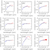 |
Fig. A.1 Obtained reflectance spectra for asteroids (39), (82), (96), (106), (175), (179), (207), (246), and (261). The blue and red parts of the merged spectra are displayed in blue and red, respectively. The SMASS reflectance spectra forthe same objects, whenever available, are shown in black. All spectra are represented after some smoothing to reduce the noise, especially at the blue and red ends. All spectra are normalised at the wavelength of 0.55 μm. |
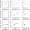 |
Fig. A.2 Same as Fig. A.1, but for asteroids (269), (588), (624), (720), (742), (808), (919), (1126), and (1214). |
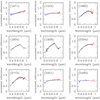 |
Fig. A.3 Same as Fig. A.1, but for asteroids (1471), (1534), (1662), (1904), (1929), (2354), (2715), (3451), and (3485). |
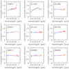 |
Fig. A.4 Same as Fig. A.1, but for asteroids (3997), (5142), (5158), (5924), (6142), (6578), (6661), and (6698), the latter having been observed independently in two different observing runs in 2010. We note that the spectrum of (3997) is certainly wrong, but it was not removed from our TNG data set for reasons explained in the text. |
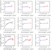 |
Fig. A.5 Same as Fig. A.1, but for asteroids (6769), (6815), (6840), (7081), (8424), (9052), (13100) (observed in two different observing runs) and (14112). We note that in the case of asteroid (13100), two independent spectra obtained during the two observing runs of October and November 2010 are superimposed in the same plot. |
Appendix B Clones of the asteroid spectra used for taxonomic classification
All clones generated for the entire set of selected parent spectra are shown in Figs. B.1–B.8. The colours usedto plot the clones in Figs. B.1–B.7 were chosen to make it easier to to identify different taxonomic classes found in this work: cyan for Class 01, dark blue for Class 02, magenta for Class 03, black for Class 04, grey for Class 05, green for Class 08, and brown for Class 09. The cases of Classes 07, 10, 11, and 12, each including all the generated clones of their parents, are shown in Fig. B.8 in dark green.
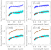 |
Fig. B.1 Parent spectra (red dots) and randomly generated clones (continues lines) for the asteroids (106), (3451), (261), and (1214). All reflectances are normalised at the same wavelength of 0.55 μm. The clones of each parent spectrum are always found to contribute mostly to one obtained taxonomic class, and are plotted superposed onto the parent spectrum. Clones found to contribute to other classes are plotted with a shift of + 0.5 in normalised spectral reflectance to distinguish them. The adopted colours in this and the following Figs. B.2–B.8 have been chosen in such a way that each obtained taxonomic class is characterised by the same colour in all plots. The exceptions are given by clones of parent spectra producing clones all belonging to one class only. These cases are shown in dark green in Fig. B.8. |
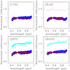 |
Fig. B.2 Same as Fig. B.1, but in the case of the clones of the TNG spectra of asteroids (175), (919), (207), and (8424). |
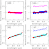 |
Fig. B.3 Same as Fig. B.1, but in the case of the clones of the TNG spectra of asteroids (6661), (5924), (96), and (1471). |
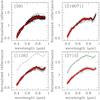 |
Fig. B.4 Same as Fig. B.1, but in the case of the clones of the TNG spectra of asteroids (39), (219071), (1126), and (2715). |
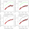 |
Fig. B.5 Same as Fig. B.1, but in the case of the clones of the TNG spectra of asteroids (179), (742), (2354), and (7081). |
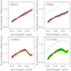 |
Fig. B.6 Same as Fig. B.1, but in the case of the clones of the TNG spectra of asteroids (624), (588), (1904), and (13100). |
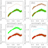 |
Fig. B.7 Same as Fig. B.1, but in the case of the clones of the TNG spectra of asteroids (808), (82), (5142), (720). |
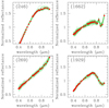 |
Fig. B.8 Same as Fig. B.1, but in the case of the clones of the TNG spectra of asteroids (246), (1662), (269), and (1929). |
References
- Belskaya, I. N., Shkuratov, Yu. G., Efimov, Yu. G., et al. 2005, Icarus, 178, 213 [NASA ADS] [CrossRef] [Google Scholar]
- Belskaya, I. N., Fornasier, S., Tozzi, G. P., et al. 2017, Icarus, 284, 30 [NASA ADS] [CrossRef] [Google Scholar]
- Binzel, R. P., DeMeo, F. E., Turtelboom, E. V., et al. 2019, Icarus, 324, 41 [NASA ADS] [CrossRef] [Google Scholar]
- Bowell, E., & Lumme, K. 1979, Asteroids, ed. T. Gehrels (Tucson, AZ: University of Arizona Press), 132 [Google Scholar]
- Bus, S. J. 1999, PhD thesis, Massachusetts Institute of Technology, MA, USA [Google Scholar]
- Bus, S., & Binzel, R. P. 2002a, Icarus, 158, 106 [CrossRef] [Google Scholar]
- Bus, S., & Binzel, R. P. 2002b, Icarus, 158, 146 [NASA ADS] [CrossRef] [Google Scholar]
- Carvano, J. M., & Davalos, J. A. G. 2015, A&A, 580, A98 [NASA ADS] [CrossRef] [EDP Sciences] [Google Scholar]
- Cellino, A., Bagnulo, S., Gil-Hutton, R., et al. 2015a, MNRAS, 451, 3473 [NASA ADS] [CrossRef] [Google Scholar]
- Cellino, A., Gil-Hutton, R., & Belskaya, I. N. 2015b, Polarimetry of Stars and Planetary Systems, eds. L. Kolokolova, J. Hough, & A. Levasseur-Regourd (Cambridge: Cambridge University Press), 360 [CrossRef] [Google Scholar]
- Cellino, A., Bagnulo, S., Belskaya, I. N., & Christou, A. 2018, MNRAS, 481, L49 [CrossRef] [Google Scholar]
- Delbò, M., Gayon-Markt, J., Busso, G., et al. 2012, Planet. Space Sci., 73, 86 [NASA ADS] [CrossRef] [Google Scholar]
- DeMeo, F. E., & Carry, B. 2013, Icarus, 226, 723 [NASA ADS] [CrossRef] [Google Scholar]
- DeMeo, F. E., Binzel, R. P., Slivan, S. M., & Bus, S. J. 2009, Icarus, 202, 160 [NASA ADS] [CrossRef] [Google Scholar]
- DeMeo, F. E., Alexander, C. M. O’D, Walsh, K. J., et al. 2015, Asteroids IV, eds. P. Michel, F. E. DeMEo, & W. F. Bottke (Tucson, AZ: University of Arizona Press), 13 [Google Scholar]
- Devogèle, M., Cellino, A., Borisov, G., et al. 2018a, MNRAS, 479, 3498 [NASA ADS] [CrossRef] [Google Scholar]
- Devogèle, M., Tanga, P., Cellino, A., et al. 2018b, Icarus, 304, 31 [NASA ADS] [CrossRef] [Google Scholar]
- Farnham, T. L., Schleicher, D. G., & A’Hearn, M. F. 2000, Icarus, 147, 180 [NASA ADS] [CrossRef] [Google Scholar]
- Gaffey, M. J., Reddy, V., Fieber-Beyer, S., & Cloutis, E. 2015, Icarus, 250, 623 [CrossRef] [Google Scholar]
- Gaia Collaboration (Prusti, T., et al.) 2016, A&A, 595, A1 [NASA ADS] [CrossRef] [EDP Sciences] [Google Scholar]
- Galluccio, L., Michel, O., & Bendjoya, Ph. 2008, AIP Conf. Ser., 1082, 165 [CrossRef] [Google Scholar]
- Gradie, J., & Tedesco, E. F. 1982, Science, 216, 1405 [NASA ADS] [CrossRef] [PubMed] [Google Scholar]
- Ivezić, Ž., Tabachnik, S., Rafikov, R., et al. 2001, AJ, 122, 2749 [NASA ADS] [CrossRef] [Google Scholar]
- Ivezić, Ž., Lupton, R. H., Jurić, M., et al. 2002, AJ, 124, 2943 [NASA ADS] [CrossRef] [Google Scholar]
- Lazzarin, M., Marchi, S., Barucci, M. A., et al. 2004, Icarus, 169, 373 [NASA ADS] [CrossRef] [Google Scholar]
- Lazzaro, D., Angeli, C. A., Carvano, J. M., et al. 2004, Icarus, 172, 179 [CrossRef] [Google Scholar]
- van Leeuwen, F., De Bruijne, J. H. J., Arenou, F., et al. 2018, Gaia DR2 documentation, European Space Agency; Gaia Data Processing and Analysis Consortium. https://gea.esac.esa.int/archive/documentation/GDR2/ [Google Scholar]
- Lumme, K., & Bowell, E. 1981, AJ, 86, 1694 [NASA ADS] [CrossRef] [Google Scholar]
- Milani, A., Cellino, A., Knežević, Z., et al. 2014, Icarus, 239, 46 [NASA ADS] [CrossRef] [Google Scholar]
- Millis, R. L., Bowell, E., & Thompson, D. T. 1976, Icarus, 28, 53 [NASA ADS] [CrossRef] [Google Scholar]
- Nathues, A. 2010, Icarus, 208, 252 [NASA ADS] [CrossRef] [Google Scholar]
- Perna, D., I., Barucci, M. A., Fulchignoni, M., et al. 2018, Planet. Space Sci., 157, 82 [NASA ADS] [CrossRef] [Google Scholar]
- Ramírez, I., Michel, R., Sefako, R., et al. 2012, ApJ, 752, 5 [NASA ADS] [CrossRef] [Google Scholar]
- Reddy, V., Sanchez, J. A., Nathues, A., et al. 2012, Icarus, 217, 153 [CrossRef] [Google Scholar]
- Reddy, V., Dunn, T. L., Thomas, C. A., et al. 2015, Asteroids IV, eds. P. Michel, F. E. DeMEo, & W. F. Bottke (Tucson, AZ: University of Arizona Press), 43 [Google Scholar]
- Sanchez, J. A., Reddy, V., Nathues, A., et al. 2012, Icarus, 220, 36 [NASA ADS] [CrossRef] [Google Scholar]
- Tanga, P., & Mignard, F. 2012, Planet. Space Sci., 73, 5 [NASA ADS] [CrossRef] [Google Scholar]
- Tedesco, E. F., Tholen, D. J., & Zellner, B. 1982, AJ, 87, 1585 [NASA ADS] [CrossRef] [Google Scholar]
- Tholen, D. J. 1984, PhD Thesis, Arizona University, Tucson, USA [Google Scholar]
- Tody, D. 1986, Proc. SPIE, 0627, 733 [NASA ADS] [CrossRef] [Google Scholar]
- Zellner, B. 1979. Asteroids, ed. T. Gehrels (Tucson, AZ: University of Arizona Press), 783 [Google Scholar]
The phase angle is the angle between the target-Sun and target-observer directions.
A description of the instrument can be found at the following URL address: http://www.tng.iac.es/instruments/lrs/
The phase angles and predicted apparent magnitudes of the targets have been computed by the public IMCCE ephemerides service available at the https://ssp.imcce.fr portal
These spectra tend to be extremely similar to one another, and for this reason we only included a representative sample of them in the analysis for cloning purposes.
All Tables
Number of clones generated for each parent spectrum, and number of them found to be members of each of the twelve taxonomic classes resulting from the classification exercise.
All Figures
|
Fig. 1 TNG spectrum of asteroid (106) Dione (blue and red curves display the original blue and red spectra before merging), with the corresponding Gaia-like synthetic spectrum obtained by converting the TNG spectrum into a discretised signal mimicking what is expected from Gaia superposed (black points), as explained in Sect. 3. |
| In the text | |
|
Fig. 2 Reflectance spectrum of asteroid (32) Pomona obtained during our 2008 observing run. The resulting reflectance spectra are significantly different, depending upon the adopted solar analogue star. One of the two spectra (corresponding to solar analogue 2, blue+red curves) is in very reasonable agreement with the SMASS spectrum of this asteroid, whereas the use of solar analogue 1 produces a quite different reflectance spectrum at all wavelengths. SA1 and SA2 correspond to solar analogue stars Hyades 64 and 61 Cyg B, respectively. |
| In the text | |
|
Fig. 3 TNG spectrum of asteroid (1929) Kollaa converted into Gaia format (red points), and surrounded by the envelope formed at each wavelength by its clones (71 in number), generated randomly using the technique described in the text. |
| In the text | |
|
Fig. 4 TNG normalised reflectance spectra of asteroids (624) Hektor, (588) Achilles, and (269) Justitia. To avoid overlapping, the spectra of (588) and (269) have been shifted by ± 0.2 with respectto the spectrum of (624). |
| In the text | |
|
Fig. 5 TNG normalised reflectance spectra of the selected asteroids whose clones are found in the resulting Class 01. Parent spectra whose clones exclusively (or the vast majority) belong to Class 01 are plotted in cyan. Parent spectra of clones mostly contributing to Class 02 are plotted in blue. Parent spectra providing only very minor contributions to Class 01 are plotted with small symbols. The black colour refers to very small numbers of clones of parent bodies mostly contributingto classes other than Class 01 or Class 02. |
| In the text | |
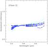 |
Fig. 6 Same as in Fig. 5, but here the reference class is Class 02. |
| In the text | |
|
Fig. 7 Spectra of clones of the spectrum of (6661) Ikemura (magenta lines), with the discretised spectra of a few clones of parent spectra (919) and (5924) superimposed, which were also found to belong to Class 03 in our taxonomy exercise. |
| In the text | |
|
Fig. 8 Spectra of clones classified in Class 05. Continuous grey lines indicate clones of the (179), (588), (624), (742), (2354), (2715), and (7081) parent spectra, whose clones are totally or predominantly found to contribute to this class. Some additional discretised spectra of a few clones of parent spectra (1126), (5142), and (13100), which are also found to be classified as Class 05, are superimposed in different colours. |
| In the text | |
|
Fig. 9 Spectra of clones classified in Class 04. Continuous black lines indicate clones of the (39), (1126) and (219071) parent spectra, whose clones are totally or predominantly found to contribute to this class. Some additional discretised spectra of a few clones of parent spectra (2354), (2715), and (7081), also found to be classified as Class 04, are superimposed in red. |
| In the text | |
|
Fig. 10 Spectra of clones classified in Class 08. Continuous green lines indicate clones of the (82), (808), and (13100) parent spectra, whose clones are totally or predominantly found to contribute to this class. Several additional discretised spectra of clones of parent spectrum (5142) are superimposed in brown, as well as a few clones of parent spectra (179), (742), and (2715), also found to be classified as Class 08, are superimposed in grey. |
| In the text | |
|
Fig. 11 Spectra of clones classified in Class 09. Continuous brown lines indicate clones of the (720), (1904), and (5142) parent spectra, whose clones are totally or predominantly found to contribute to this class. Some additional discretised spectra of clones of parent spectra (82) and (808) are superimposed in green, while a few clones of parent spectra (261) and (1214), also found to be classified as Class 09, are superimposed in cyan. |
| In the text | |
|
Fig. A.1 Obtained reflectance spectra for asteroids (39), (82), (96), (106), (175), (179), (207), (246), and (261). The blue and red parts of the merged spectra are displayed in blue and red, respectively. The SMASS reflectance spectra forthe same objects, whenever available, are shown in black. All spectra are represented after some smoothing to reduce the noise, especially at the blue and red ends. All spectra are normalised at the wavelength of 0.55 μm. |
| In the text | |
|
Fig. A.2 Same as Fig. A.1, but for asteroids (269), (588), (624), (720), (742), (808), (919), (1126), and (1214). |
| In the text | |
|
Fig. A.3 Same as Fig. A.1, but for asteroids (1471), (1534), (1662), (1904), (1929), (2354), (2715), (3451), and (3485). |
| In the text | |
|
Fig. A.4 Same as Fig. A.1, but for asteroids (3997), (5142), (5158), (5924), (6142), (6578), (6661), and (6698), the latter having been observed independently in two different observing runs in 2010. We note that the spectrum of (3997) is certainly wrong, but it was not removed from our TNG data set for reasons explained in the text. |
| In the text | |
|
Fig. A.5 Same as Fig. A.1, but for asteroids (6769), (6815), (6840), (7081), (8424), (9052), (13100) (observed in two different observing runs) and (14112). We note that in the case of asteroid (13100), two independent spectra obtained during the two observing runs of October and November 2010 are superimposed in the same plot. |
| In the text | |
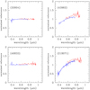 |
Fig. A.6 Same as Fig. A.1, but for asteroids (33804), (43962), (49833), and (219071). |
| In the text | |
|
Fig. B.1 Parent spectra (red dots) and randomly generated clones (continues lines) for the asteroids (106), (3451), (261), and (1214). All reflectances are normalised at the same wavelength of 0.55 μm. The clones of each parent spectrum are always found to contribute mostly to one obtained taxonomic class, and are plotted superposed onto the parent spectrum. Clones found to contribute to other classes are plotted with a shift of + 0.5 in normalised spectral reflectance to distinguish them. The adopted colours in this and the following Figs. B.2–B.8 have been chosen in such a way that each obtained taxonomic class is characterised by the same colour in all plots. The exceptions are given by clones of parent spectra producing clones all belonging to one class only. These cases are shown in dark green in Fig. B.8. |
| In the text | |
|
Fig. B.2 Same as Fig. B.1, but in the case of the clones of the TNG spectra of asteroids (175), (919), (207), and (8424). |
| In the text | |
|
Fig. B.3 Same as Fig. B.1, but in the case of the clones of the TNG spectra of asteroids (6661), (5924), (96), and (1471). |
| In the text | |
|
Fig. B.4 Same as Fig. B.1, but in the case of the clones of the TNG spectra of asteroids (39), (219071), (1126), and (2715). |
| In the text | |
|
Fig. B.5 Same as Fig. B.1, but in the case of the clones of the TNG spectra of asteroids (179), (742), (2354), and (7081). |
| In the text | |
|
Fig. B.6 Same as Fig. B.1, but in the case of the clones of the TNG spectra of asteroids (624), (588), (1904), and (13100). |
| In the text | |
|
Fig. B.7 Same as Fig. B.1, but in the case of the clones of the TNG spectra of asteroids (808), (82), (5142), (720). |
| In the text | |
|
Fig. B.8 Same as Fig. B.1, but in the case of the clones of the TNG spectra of asteroids (246), (1662), (269), and (1929). |
| In the text | |
Current usage metrics show cumulative count of Article Views (full-text article views including HTML views, PDF and ePub downloads, according to the available data) and Abstracts Views on Vision4Press platform.
Data correspond to usage on the plateform after 2015. The current usage metrics is available 48-96 hours after online publication and is updated daily on week days.
Initial download of the metrics may take a while.