| Issue |
A&A
Volume 642, October 2020
|
|
|---|---|---|
| Article Number | A203 | |
| Number of page(s) | 29 | |
| Section | Interstellar and circumstellar matter | |
| DOI | https://doi.org/10.1051/0004-6361/202038088 | |
| Published online | 20 October 2020 | |
Spectroscopic study of the HII regions in the NGC 1232 galaxy
1
NAT – Universidade Cidade de São Paulo/Universidade Cruzeiro do Sul,
Rua Galvão Bueno 868,
São Paulo
01506-000, Brazil
e-mail: This email address is being protected from spambots. You need JavaScript enabled to view it.
2
Laboratório Nacional de Astrofísica,
Rua Estados Unidos 154,
Itajubá-MG
37530-000, Brazil
Received:
3
April
2020
Accepted:
19
August
2020
Abstract
Context. NGC 1232 is a face-on spiral galaxy that serves as an excellent laboratory for the study of star formation due to its proximity. Recent studies have revealed interesting features about this galaxy: X-ray observations suggest that it recently collided with a dwarf galaxy, however, no apparent remnant is observed.
Aims. In this study, we search for evidence of this possible collision.
Methods. We used long-slit optical spectra of the galaxy in two different positions obtained with the Goodman spectrograph at the SOAR telescope.
Results. We detected 18 HII regions in the north-south direction and 22 HII regions in the east-west direction and a background galaxy, NGC 1232B, for which we present the first redshift measurement and spectral analysis. We used the stellar population fitting technique to study the underlying stellar population of NGC 1232 and NGC 1232B and to subtract it from the spectra to measure the emission lines. The emission lines were used to determine the extinction, electron density, chemical abundance, and the star-formation rate gradient of NGC 1232.
Conclusions. As is common in spiral galaxies, we found a stellar population gradient with older populations at the central regions and younger ones towards the outskirts, along with a negative oxygen abundance gradient of −0.16 dex/re. Due to the difficulty of measuring important emission lines, the number of objects for the abundance gradient is small, but there is a hint that this galaxy has a broken gradient profile, with a drop towards the center. Some authors have explained this effect as the result of a satellite collision, but observations of a large sample of spiral galaxies shows evidence that goes against such a mechanism. If the collision caused any disturbance in the galaxy, we believe it would be small and hard to detect with a limited number of objects. From all the other measurements, we found no deviations from a typical spiral galaxy and no significant difference between different directions in the galaxy. The stellar population and emission line analysis of NGC 1232B suggest that it is a starburst galaxy.
Key words: ISM: abundances / HII regions / galaxies: individual: NGC 1232 / galaxies: individual: NGC 1232B / galaxies: star formation
© ESO 2020
1 Introduction
Spiral galaxies are the most numerous type of galaxy in the Local Universe and are where most star formation occurs (Brinchmann et al. 2004). Understanding the formation and evolution of these systems is crucial for understanding how stars form in galaxies. Chemo-dynamical models have made important progress in understanding these complex systems, agreeing, for example, on a local dependence of the star formation law, despite the possibility of other factors affecting the star formation rate (SFR) over galactic scales (e.g. Schmidt 1959; Dopita 1985; Kennicutt 1989; Wyse & Silk 1989; Dopita & Ryder 1994; Prantzos & Aubert 1995). It has been proposed that an inside-out growth of the disc as a result of the increased timescales of gas infall with radius leads to a radial dependence on the SFR (Matteucci & Francois 1989; Boissier & Prantzos 1999). The importance of other processes, such as metal-rich outflows (e.g. Mac Low & Ferrara 1999) or radial gas flows (e.g. Edmunds & Greenhow 1995; Lacey & Fall 1985) is more controversial. In a recent review, Sánchez (2020) constructed the largest dataset of resolved nearby galaxies. By combining his analysis with others published in recent papers, he concluded that the evolution of galaxies is mainly shaped by local properties but it is also influenced to some extent by global ones. The star formation and chemical enrichment in galaxies, along with their enhancement and quenching, follow local evolutionary laws that are also verified at kiloparsec scales. He argues that recycling, inflows, and outflows that influence how the SFR shapes the chemical enrichment happens more on local rather than global scales. One of the strongest constraints for the main parameters in chemical evolution models is the spatial distribution of chemical abundances (Koeppen 1994; Edmunds & Greenhow 1995; Tsujimoto et al. 1995; Mollá et al. 1996, 1997; Prantzos & Boissier 2000; Chiappini et al. 2001; Mollá & Díaz 2005; Fu et al. 2009; Pilkington et al. 2012).
Nebular emission lines have been one of the main tools used to study the complex physical processes at play in spiral galaxies and their connection with the galaxy’s chemical abundances. In particular, the emission line spectra of extragalactic HII regions trace the young, massive star components and they have become fundamental to investigate abundances in galaxies.
While statistical studies with large sample of galaxies can help us to understand the role and importance of many mechanisms in general, the detailed study of individual, nearby objects can reveal important information about the mechanisms at play.
In this sense, NGC 1232 is an almost face-on (i ≈ 30°) gas-rich spiral galaxy morphologically classified as SAB(rc)c. It has a weak bar at its core, a small bulge, and long arms that disperse to the outer regions, producing a remarkable number of thin arms. These arms produce a well-defined, though somewhat unusual spiral pattern, as they do not bend smoothly as might be expected of such a galaxy. They bend more abruptly, which Arp (1982) suggested tobe a distortion caused by a previous interaction with another galaxy. Due to its frontal position, its proximity (19.8 Mpc1) and becauseit has numerous star-forming regions, NGC 1232 is considered an excellent laboratory for the study of star formation.
Quite nearby in the sky projection, there is another galaxy, NGC 1232A. However, because of the strong difference in redshift between them (z = 0.00535 for NGC 1232 and z = 0.02201 for NGC 232A2), they are notcurrently interacting and have probably never interacted before. Radio studies indicate that NGC 1232 has a large neutral gas envelope that extends far beyond the optical limit of the galaxy (van Zee & Bryant 1999). The nuclear region is dominated by an older stellar population (Martins et al. 2013), while the spiral arms are populated by numerous star-forming regions.
Diffuse X-ray observations from the Chandra Space Telescope suggest that NGC 1232 has recently collided with a dwarf galaxy, however, there is no apparent remnant of this event. According to Garmire (2013), the shock wave produced by this collision may have caused the formation of massive bright stars. High-resolution imaging studies in Hα employed tomeasure the star formation rate (SFR) in NGC 1232, reinforce this hypothesis. According to de Souza et al. (2018), there is a significant number of luminous HII regions in the northern and eastern regions as well as an excess of star formation in the northeast region of the galaxy. This finding is important because the frequency of the collisions between large spirals and dwarf galaxies is difficult to estimate and most galaxies show no signs of such collisions. At earlier times, these collisions were probably very frequent, and contributed significantly to galaxy growth. If the X-ray excess is confirmed as an evidence of this type of collision, this may be a way to estimate the frequency of collision with dwarf galaxies and how much such collisions contribute to the galaxy growth and evolution in the current epoch (Garmire 2013).
In this work, we present the most detailed study of the HII regions of NGC 1232 using long-slit spectroscopy, with slits positioned along the north-south and east-west directions. This allows us to carry out a study of the spatial variation of their properties along these two axis of the galaxy.
This paper is organised as follows: in Sect. 2, we describe the observations, data reduction, and HII regions detections. In Sect. 3, we use the spectral fitting technique to remove the underlying stellar population in order to measure the emission lines. The spectral fitting also gives us information about the stellar population gradient of the galaxy. In Sect. 4, we describe the emission line measurements and in Sect. 5, we use these emission lines to characterise the HII regions in the galaxy and describe results for the background galaxy NGC 1232B (first spectroscopic observation of the galaxy). In Sect. 6, we determine the chemical abundance of the HII regions and in Sect. 7, the star formation gradient of the galaxy. In Sect. 8, we present our discussion and conclusions.
2 Observations, data reduction, and HII region detection
2.1 Observations and data reduction
In order to study the properties of the HII regions of NGC 1232, we observed the galaxy with the Goodman spectrograph at SOAR telescope on the night of 2 October 2017 and 5 February 2018. We used the 0.84″ wide slit mode and diffraction grating of 400 l mm−1, with the slit oriented in two different positions: north-south (N-S − blue camera) and east-west (E-W − red camera). The charege-coupled device (CCD) that we used has a spatial scale of 0.15 arcsec pixel−1, and provides spectral coverage from 3700 to 7200 Å. The spectral resolution R is ≈1000 at 5500 Å. The CCD binning was set to 1×1 yielding a spatial scale of 0.15 arcsec pixel−1. Three individual on-source integrations were carried out for each slit, with exposure times of 20 min each. The seeing was 0.6−0.8″ on 2 October and 0.8− 1.0″ on 5 February, both with photometric skies.
The data were reduced in a standard manner using the Image Reduction and Analysis Facility (IRAF) software3. It includes bias subtraction, division by a normalised flat field, wavelength calibration using a HeNeAr lamp for the dispersion solution, and flux calibration. In this last step, observation of a Pilkington et al. (2012) standard star, taken the same night, was employed. Moreover, atmospheric extinction correction was applied to each spectrum using the CTIO coefficients available in IRAF using the tasks SEN-S FUNC and CALIBRATE.
2.2 HII region detection
The spatial coverage of long slits allows for the detection of HII regions from the center of the galaxy to its edges. Through the identification of Hα emission peaks along the slit, 22 HII regions were detected in the E-W direction and 18 in the N-S direction, plus a background galaxy called NGC 1232B by Arp (1982). Table 1 presents basic information about the apertures used for the extractions with their respective distances from the center of the galaxy. In the N-S slit, apertures 1 to 7 are nuclear apertures, 8 to 12 are in the north direction, and 13 to 18 in the south direction. Aperture 19 refers to NGC 1232B. In the E-W slit, the apertures 1 to 4 and 14 to 16 are in the nuclear region, 17 to 21 refer to the eastern region, and 5 to 13 to the western region of galaxy. It is important to mention that in the nuclear apertures in both directions, the emission corresponds to the emission of the nucleus and the bulge, and it is not possible to disentangle individual HII regions there. We ensured that the number of pixels summed in each extraction window (from 20 to 50 pixels) corresponded to a window much larger than the seeing, which gives a physical meaning to each extraction.
Figure 1a shows an Hα image of NGC 1232 (de Souza et al. 2018), where the N-S and E-W apertures are represented by white lines. Figure 1b shows the spatial distribution of light in each slit and the peaks where the HII regions and NGC 1232B were extracted. The spectra of these extractions are shown in Fig. 2 for the N-S slit and in Fig. 3 for the E-W slit. The spectrum of NGC 1232B is shown and discussed in Sect. 5.
3 Stellar population analysis and subtraction
The typical spectrum of an HII region is dominated by intense emission lines, with very weak or no underlying stellar continuum. However, our observations were made using a long slit that did not necessarily encompass strictly the HII regions. To make sure that contamination from the underlying stellar population does not alter the emission line measurements we used the spectral fitting technique to remove its contribution.
For this purpose, we used the code STARLIGHT (Cid Fernandes et al. 2004, 2005a; Mateus et al. 2006; Asari et al. 2007). This code fits the observed integrated spectrum of a given stellar population with a combination, in different proportions,of single stellar populations with different ages and metallicities. To be sure that the patterns found here are not the result of a particular choice of models, we tested two different bases of models: Bruzual & Charlot (2003, hereafter BC03), and Vazdekis et al. (2015, hereafter V15). Using STARLIGHT, the internal kinematics is determined simultaneously with the population parameters. Extinction is also modeled by STARLIGHT as due to a dust screen and parameterised by the V -band extinction (AV). We use the Cardelli et al. (1989) extinction law. The emission lines have been masked for the fit. Figure 4 shows, as an example of the stellar population fitting, the results for apertures 01 (nuclear) and 13 (southern region), both from the N-S slit. Results for all the apertures can be found in Appendix A.
Although the main purpose of the spectral fitting in this paper is the removal of the underlying stellar population for the measurement of the emission lines, there is information in the fit that deserves some analysis. Here, it is important to point out that it has been shown that results for the stellar population fitting technique can be trusted only in spectra with S∕N = 10 or larger (Cid Fernandes et al. 2005a). Because of this, we excluded from this analysis all the spectra with a signal-to-noise ratio (S/N) below 10. For the E-W direction this was more problematic, as all of the outer spectra are very noisy.
To perform this analysis, we used the condensed population vector as defined by Cid Fernandes et al. (2005b), which combines the stellar populations taking into account noise effects between similar spectral components. The stellar population is binned into categories and represented by the vectors xY : t ≤ 5 × 10⁷ yr (young population), xI: 1 × 10⁸ ≤ t ≤ 2 × 10⁹ yr (intermediate age population) and xO: t ≥ 2 × 10⁹ yr (old population), where t is the age of the stellar population. These results are presented in Tables 2 (N-S slit) and 3 (E-W slit). Additional results, namely the extinction value AV, the mean age ⟨log (tav)⟩, and mean metallicity ⟨Zav⟩ of the stellar population, weighted by the light fraction, are also presented. These last two quantities are defined through Eqs. (1) and (2):
 (1)
(1)
 (2)
(2)
where N* is the number of SSPs used in the base.
The quality of the fits is measured by the reduced χ2 and the adev parameter, which represents the deviation average percentage over all adjusted pixels, determined by:
 (3)
(3)
where Oλ is the observed spectrum and Mλ the model fitted to this spectrum. From the values of χ2 and adev in Tables 2 and 3 it can be seen that the outermost apertures, which have very low S/N, have results with very large errors that cannot be trusted.
Figures 5 and 6 show the variation of the age vectors as a function of the distance to the nucleus, for the N-S and E-W directions, respectively. Results from BC03 and V15 are in agreement and basically present the same trends. This gives us more confidence in the results. These figures show an important difference between the N-S and E-W directions: in the N-S direction, the central region presents an older population, becoming younger away from the nucleus. For the E-W slit, the stellar population of the central HII regions is much younger, and although there is still a trend of becoming even younger to the external regions, the variations are much smaller. To be sure this was not a spurious result due to the lower S/N of the spectra, specially in the blue, we tested the technique restricting the wavelength to 4300–7200 Å (without the blue part). The results were virtually the same (changes of less than 6% in the young population vector).
We believe the difference between the N-S and E-W slits is related to the position of the slit: the N-S slit was positioned slightly off the central luminosity peak of the galaxy, as can be seen in Fig. 1. This was done on purpose, so that the galaxy NGC 1232B would fall in the slit. The E-W slit, however, is placed exactly through the central luminosity peak. Besides that, the brightest part of NGC 1232 nucleus seems to be more extended in the E-W direction than in the N-S direction, perhaps due to the presence of a small bar in this direction. This behavior (older population in the nucleus and a gradient towards younger population outwards) is typical of disc galaxies (Sánchez-Blázquez et al. 2014).
Detected HII Regions and NGC 1232B.
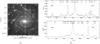 |
Fig. 1 (a) Hα image of NGC 1232 from de Souza et al. (2018). The white lines represent the slits from where the HII regions were extracted along the N-S and E-W directions. (b) Spatial distribution of flux in Hα of the slits N-S (top) and E-W (bottom), showing the peaks which correspond to each HII region (and NGC 1232B) extracted. The numbers on top correspond to their names in Table 1 and the size of the extraction of each HII regions is shown by the ranges below these numbers. |
4 Emission lines
4.1 Flux measurements
After the subtraction of the underlying stellar population, the emission lines were measured. The measurements were made with a multi-component fit, using single Gaussians per emission line, plus a linear function for the continuum. We chose to subtract the synthetic spectra obtained using BC03, because the S/N after subtraction is higher than that of V15. Emission lines are detected in all apertures, although in the nucleus and circumnuclear regions they are particularly weak since the spectra are dominated by the stellar light. For some apertures, only Hα and [NII] were identified. Table 4 presents the measured fluxes for both slits.
4.2 Extinction
The interstellar extinction was calculated using the Balmer decrement measured by Hα and Hβ, and the reddening law of Cardelli et al. (1989), assuming a total-to-selective extinction ratio RV = AV/EB−V = 3.1, and case B theoretical ratios at 10 000 K (Osterbrock & Ferland 2006). We calculated the extinction coefficient c for each HII region using the ratio Hα/Hβ, as defined by Eq. (4), when both lines were measured:
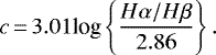 (4)
(4)
The values obtained for each HII region are presented in Table 5. The errors were estimated through a Monte Carlo simulation, varying the fluxes within the errors a thousand times.
Figure 7 shows the variation of the calculated extinction coefficient as a function of the distance to the galaxy center. We also include in this figure the extinction coefficients obtained by Bresolin et al. (2005), who measured line fluxes of 13 metal-rich HII regions in NGC 1232 (open symbols in this figure). From their 13 objects, we considered 2 to the north (objects 05 and 08 in their paper), 1 to the south (object 14 in their paper), and 2 to the east (objects 10 and 11 in their paper), which were the objects included in this figure. The other 8 objects were located at different regions in the galaxy and were not included in this plot.
Trends of decreasing extinction towards the outskirts of spiral galaxies are typically reported (e.g. van Zee et al. 1998). However, our data shows that both the N-S and E-W directions show no extinction gradient. The absence of a extinction gradient for NGC 1232 was also found in Bresolin et al. (2005). However, we note that the E-W regions seem to have, on average, smaller extinction than the ones from N-S, at least outside the nucleus.
With the calculated extinction coefficient, it was possible to correct the emission line fluxes by the extinction effect using the extinction law from Cardelli et al. (1989). Dereddened fluxes for the HII regions where extinction could be derived are also presented inTable 5. All the further analysis in this paper is done using the extinction-corrected line fluxes.
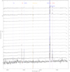 |
Fig. 2 Spectra of HII regions from the N-S slit. The dotted lines in red and blue mark the main emission lines detected. Dotted orange lines mark artificial effects due to to instrumental problems. The numbers on the right side of the plot identify the apertures. |
4.3 Comparison with the literature
Previous works have obtained spectra of HII regions of NGC 1232, but they were mostly targeted at bright regions in the outskirts of the galaxy. We found two works that have HII regions in common with our objects, van Zee et al. (1998) and Bresolin et al. (2005), with two regions in each. We compare the fluxes of the brightest lines of these objects in Fig. 8, where [OIII]λ5007 correspond to the red points, [NII]λ6583 the blue points, and [SII]λ6716 and [SII]λ6731 to the green points. We note that the data from van Zee et al. (1998) come from low-resolution spectroscopy and many of their measurements are actually a blend of two lines: [OIII]λ4959+5007, [NII]λ6548+6583 and [SII]λ6716+6731. The resulting comparison displays the reddening-corrected line intensities (in units of Hβ = 100) from this work (horizontal axis) with the literature values (vertical axis). We can see from this figure that there is no evidence for systematic deviations from the dashed line, which represents the location for equal values. Considering the effects of varying slit apertures, orientation, and centering of the objects, the agreement is excellent.
5 Empirical diagrams
Diagrams of a number of crucial line ratios can be used to assess general properties of the extracted HII regions. For example, Fig. 9 shows the density-sensitive ratio [SII]λ6716/[SII]λ6731 as a function of the distance to the galaxy center. The dashed line in this figure represents the “zero-density” limit reached by this line ratio, for Te = 10 000 K, which is 1.43. Values of 9 of the 13 HII regions of Bresolin et al. (2005) were plot as open symbols for comparison. The other 4 objects have very large distances from the nucleus (r > 170″). What can be seen in this figure is that most of the objects lie close to the ratio limit, meaning densities of tens to a few hundred particles per cm3.
To determine the electron density for each HII region we used the recipe from Proxauf et al. (2014). They recalculated some well-known diagnostic diagrams using the photoionisation code CLOUDY (Ferland et al. 2013) and developed a simpler analytical expression to determine the electron density than the traditional nonlinear equations (McCall et al. 1985). The equation for electron density is based on [SII] lines such that:
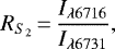 (5)
(5)
and the electron density according to Proxauf et al. (2014) is given by:
![Mathematical equation: \begin{eqnarray*} \log(n_{\textrm{e}}[\textrm{cm}^{-3}]) &\,{=}\,& 0.0543 \tan (-3.0553R_{S_2}+2.8506) \nonumber \\ &&+ 6.98 - 10.6905 R_{S_2} \nonumber \\ &&+ 9.9186R^2_{S_2} - 3.5442R^3_{S_2}.\end{eqnarray*}](/articles/aa/full_html/2020/10/aa38088-20/aa38088-20-eq6.png) (6)
(6)
The values obtained for the electron density in each HII region, as well as for NGC 1232B are presented in Table 6. Figure 10 shows the density as a function of the distance to the nucleus of the galaxy. Again here we plot the HII regions from Bresolin et al. (2005) for comparison. For the objects where the  was larger than the theoretical limit of 1.43, we assumed a lower limit of ne = 10 cm−3, and for two objects, where the ratio was too small and Eq. (11) was not valid anymore, we assumed an upper limit of ne = 10 000 cm−3.
Gutiérrez & Beckman (2010) found that the density of the HII regions of the galaxies M51 and NGC 4449 tended to decrease with galactocentric distance, with scale lengths similar to the column densities of HI. In its first approximation, it would indicate that the HII regions can be considered in pressure equilibrium with the surrounding environment. Figure 10 shows the same tendency for the HII regions of this work if the upper limits are ignored. The possible exception is region 17 of the N-S slit (region to the south, which is at a distance of 68″ from the nucleus and has a density of about 1000 cm−3). These authors found that for the two galaxies studied the electron density variation with galactocentric distance can be very well described by an exponential function in the form of:
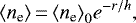 (7)
(7)
where ⟨ne⟩0 is a central value of the electron density and h is a scale-length. We have a much smaller number of HII regions than Gutiérrez & Beckman (2010), but fitting this equation to our data (not considering the upper and lower density limits and taking the error bars into consideration) returns values of ⟨ne⟩0 = 524 ± 53 cm−3 and h = 7.97 ± 0.99 kpc. This fit is represented by the dotted line in Fig. 10. We can also include the data from Bresolin et al. (2005) in the fit, which then returns the values ⟨ne⟩0 = 510 ± 55 cm−3 and h = 8.62 ± 1.16 kpc. The two fitsare very similar. This is represented by the dashed line in this figure. Gutiérrez & Beckman (2010) found a scale-length of 9 kpc for M51 and 11 kpc for NGC 4449. For M51, the density scale-length is the same as the HI scale-length measured by Tilanus & Allen (1991). They did not have the HI scale-length of NGC 4449, but they argue that since the HI galaxy radius of M51 is 15 kpc and of NGC 4449 is 18 kpc, by comparison they could also claim that the electron densities in the HII regions follow the column density of the HI gas for this galaxy too. NGC 1232 is much larger than these galaxies, and its estimated HI radius is about 37 kpc (van Zee & Bryant 1999). If we follow the same argument, we can say that in the case of NGC 1232, the electron densities of these regions are not correlated with the column density of the HI gas. On the other hand, as mentioned in the introduction, NGC 1232 has an extended envelope, which might be the result of a collision with a dwarf galaxy. In this case, the current radius of the HI might not be representative of the HI scale length. So this conclusion has to be taken with a grain of salt.
Diagnostic diagrams like the ones presented in Fig. 11 can be used to study the excitation properties of the HII regions. These diagrams relate the low excitation lines [NII]λ6583/Hα and [SII]λ6716,6731/Hα with a high excitation one, namely, [OIII]λ5007/Hβ. Again, we added the data from Bresolin et al. (2005) to the plot for comparison, with open symbols. Although for all our regions with emission lines, the [NII]λ6583/Hα was measured, and for most of them, the [SII]λ6716,6731/Hα was also measured, it was only possible to measure the [OIII]λ5007/Hβ line for a few of them. This already hints that these are low-excitation objects. For the few where the [OIII]λ5007/Hβ line was measured, this is confirmed. These objects lie in the low excitation part of the diagram, where the theoretical boundaries from Dopita et al. (2000) are plotted (full red lines). High-excitation objects would be found in the upper part of this diagram, where the line turns sharply to the left.
There are two points outside the region associated with star-forming objects: region 1 of the N-S slit and region 14 of the E-W slit. These are two apertures very near the center of the galaxy, where the stellar population dominates the spectra. There might be two reasons for the location of these points in this figure: the Hα and Hβ lines are seen in absorption before the stellar population subtraction. It is very possible that the model fitted to the underlying stellar population is underestimating these lines, artificially making the line ratios larger. If, however, we believe the models are correct, it would mean the line excitation in this regions have contribution of other mechanisms besides hot stars, such as shocks, for example (potentially induced by the recent merger with a dwarf). We discard the possibility of an AGN contribution to the emission lines because neither the evidence found here nor that already reported in the literature (in other wavelength intervals) suggest the presence of an active nucleus in the center of this object.
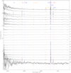 |
Fig. 3 Spectra of HII regions from the E-W slit. The dotted lines in red and blue mark the main emission lines detected. Dotted orange lines mark artificial effects due to instrumental problems. The numbers to the right side of the plot identify the apertures. |
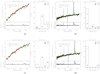 |
Fig. 4 Example of the stellar population spectral fitting. (a) and (c): aperture 01 (nucleus of the galaxy, N-S slit) fitted with BC03 and V15 models, respectively, and (b) and (d): aperture 13(N-S slit), also fitted with BC03 and V15 models, respectively. In each figure, top left panel: observed spectrum inblack, and the fitted synthetic spectrum in red. The regions marked in green represent masked intervals, ignored by STARLIGHT because of the presence of emission lines. Bottom left panel: residual of the difference between the two. Right panel: star formation history (SFH), which means the contribution of each population age and metallicity to the final synthetic spectrum. |
Results of the stellar population fitting for the HII regions of the N-S slit and NGC 1232B.
NGC 1232B
The galaxy NGC 1232B was first cited by Arp (1982) with no further information in the literature beyond the image in this paper. The positioning of the slit in the N-S direction allowed us to include this object and thus obtain its spectrum, as shown in Fig. 12. As can be seen in this figure, the spectrum shows strong emission lines. Using these lines. we measured a redshift of z = 0.09261. To the bestof our knowledge, this is the first report of the measurement of z for this object.
In order to measure the emission line fluxes, we followed the same procedure for the HII regions in NGC 1232. That is, fitting the stellar continuum with STARLIGHT, subtraction of the stellar population, and Gaussian fitting of the line profiles. Table 5 lists the line emission fluxes.
As for the HII regions, we obtained the extinction coefficient through the Hα and Hβ line ratio. The galaxy does not seem to be very dusty, with c(Hβ) ≈0.85, close to that found for the HII regions.
The stellar population fitting of the spectrum reveals it is dominated by a young stellar population, as can be seen in Fig. 13.
We also estimated the galaxy’s abundance using the bright line method values from N2 and O3 N2 (see next section for definitions), which are presented in Table 6, as well as the abundances derived from these. The results indicate that the abundance of the galaxy is close to the solar value. We can also use the emission lines measured for NGC 1232B for ionisation source diagnostics.
The green dot in Fig. 11 represents NGC 1232B. Its place in the diagram indicates the ionisation due to stars, which is also supported by the stellar population fitting. To classify this galaxy as a starburst, we adopt the criteria from Bergvall et al. (2016), based on the Hα emission line equivalent width (E-W), its FWHM (full width at half maximum) and a relation between the [OIII] and [NII] emission lines, namely:
-
EWHα ≥ 60 Å,
-
FWHMHα ≤ 540 km s−1,
-
log([OIII]λ5007/Hβ) < 0.71/log([NII]λ6584/Hα-0.25) + 1.25.
From the measured Hα emission line of NGC 1232B, we obtained EW = 803 Å and a FWHM of 320 km s−1. From the measured [OIII] and [NII] lines, we obtained log([OIII]λ5007/ Hβ) = 0.09 and 0.71/log([NII]λ6584/Hα-0.25)+1.25 = 0.58. This means that NGC 1232B satisfies all the necessary criteria for it to be considered a starburst galaxy.
Results of the stellar population fitting for the HII regions of the E-W slit.
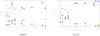 |
Fig. 5 Stellar population gradient for the N-S slit of NGC 1232, obtained with BC03 models (a) and V15 models (b). Triangles represent the southern region and circles the northern region. |
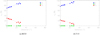 |
Fig. 6 Stellar population gradient for the E-W slit of NGC 1232, obtained with BC03 models (a) and V15 models (b). Triangles represent the western region and circles the eastern region. |
Emission line fluxes for the N-S and E-W apertures of NGC 1232 and for NGC 1232B.
Reddening corrected emission line fluxes (relative to Hβ) for the N-S and E-W slits.
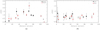 |
Fig. 7 Extinction coefficient as a function of distance to the nucleus of the galaxy NGC 1232, for the N-S (a) and E-W (b) slit. Open symbols in both figures are the HII regions from Bresolin et al. (2005). |
 |
Fig. 8 Comparison of reddening-corrected line intensities (in units of Hβ = 100), of the most common lines, measured in the current work (horizontal axis) and values from the literature (vertical axis). Red points refer to [OIII]λ5007, blue points to [NII]λ6583 and green points to [SII]λ6716 and [SII]λ6731. |
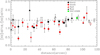 |
Fig. 9 Density-sensitive diagnostic diagram using the line ratio [SII]λ6716/[SII]λ6731 as a function of the distance to the galaxy nucleus. Open symbols are data from Bresolin et al. (2005). Colors and symbols are the same as for our data, and open gray squares are the HII regions that are in a different direction than the ones covered by our slits. |
6 Abundance from statistical methods
Studying the chemical composition of spiral galaxies is an important tool in improving our knowledge of the evolution of these complex systems. Optical emission lines can be used to determine ionic abundances of many key elements, but their line emissivities strongly depend on the electron density and temperature of the gas. The electron temperature can be obtained through line ratios involving auroral lines (like [OIII]λ4363 or [NII]λ5755), which is a major obstacle for extragalactic HII regions. These lines are intrinsically weak, and because the cooling efficiency of the gas increases with the gas abundance, they become too faint to be observed with the largest telescopes even at modest metallicities. In these cases, it is still possible to obtain estimates of nebular abundances through an alternative method using only the intensity of the brightest emission lines. This method is called an “empirical” or “semi-empirical” approach, or, more descriptively, the “bright lines” method (Dinerstein 1990). This method has many applications besides extragalactic HII regions and it has been used in chemical abundance studies of a variety objects, such as low surface-brightness galaxies (Kuzio de Naray et al. 2004)and star-forming galaxies at intermediate and high redshifts (Kobulnicky & Kewley 2004; Shapley et al. 2004; Sanders et al. 2020).
The lines ([OII]3727Å+ [OIII]4959,5007Å) were first calibrated and used as an abundance indicator by Pagel et al. (1979) and have since been recalibrated many times. Variations of these lines and combinations with other lines of [NII], [SII], and [SIII] were also adopted (McCall et al. 1985; Mathis 1985).
The most common abundance indicators using the bright-line method in the literature are:
![Mathematical equation: \begin{equation*} R_{23}\,{=}\,\frac {\mathrm{[OII}] \lambda 3727+\mathrm{[OIII]} \lambda 4949,5007}{\mathrm{H\beta}}, \label {eq4.3} \end{equation*}](/articles/aa/full_html/2020/10/aa38088-20/aa38088-20-eq9.png) (8)
(8)
![Mathematical equation: \begin{equation*} S_{23}\,{=}\,\frac{\mathrm{[SII}] \lambda 6716, 6731 +\mathrm{[SIII]} \lambda 9069, 9532}{\mathrm{H\beta}}, \label {eq4.4} \end{equation*}](/articles/aa/full_html/2020/10/aa38088-20/aa38088-20-eq10.png) (9)
(9)
![Mathematical equation: \begin{equation*} N_2\,{=}\,\textrm{log}\frac { \mathrm{[NII]} \lambda 6583}{\mathrm{H\alpha}}, \label {eq4.5} \end{equation*}](/articles/aa/full_html/2020/10/aa38088-20/aa38088-20-eq11.png) (10)
(10)
![Mathematical equation: \begin{equation*} O_3N_2\,{=}\,\textrm{log} \frac {(\mathrm{[OIII]}\lambda 5007 / \mathrm{H\beta})}{(\mathrm{[NII]} \lambda 6583/\mathrm{H \alpha)}}, \label {eq4.6} \end{equation*}](/articles/aa/full_html/2020/10/aa38088-20/aa38088-20-eq12.png) (11)
(11)
which were defined by Pagel et al. (1979, Eq. (8)), Díaz & Pérez-Montero (2000, Eq. (9)), Denicoló et al. (2002, Eq. (10)), Alloin et al. (1979) and Pettini & Pagel (2004, Eq. (11)).
In this work, it was not possible to calculate R23 because of the weak oxygen line at 3727 Å that we were not able to measure. Also, the lines necessary for the S23 are out of range of our spectra. We then use the N2 and O3 N2 indexes to estimate the abundances. It’s important to be aware, however, that these indexes might also be sensitive to the ionisation parameter and not only to the metallicity (Poetrodjojo et al. 2018). These values are presented in Table 6. We used these indexes to obtain the oxygen abundances, adopting the calibration from Marino et al. (2013). These authors recalibrated these indexes using Te based abundances from 603 HII regions extracted from the literature, together with new measurements from the CALIFA survey (Sánchez et al. 2012). They obtained:
 (12)
(12)
and
 (13)
(13)
The oxygen abundance values obtained for each HII region from these indexes are presented in Table 6. To derive a radial distribution of abundances that can be compared with values from the literature, we used the galactocentric distances normalised by the disc effective radius (re). This parameter was obtained from its relation with the disc scale-length (rd) as suggested by Sánchez et al. (2014): re = 1.67835 rd. We derived the disc scale-length from the surface brightness profile of NGC 1232 using its g-band image from de Souza et al. (2018). This profile was fitted with the classical exponential decline from Freeman (1970):
 (14)
(14)
where  is the extrapolated central surface brightness and rd the scale-length of the disc. For NGC 1232, we found rd = 28.6″, which gives re = 48.0″ (or 5.3 kpc).
Figures 14 and 15 show the oxygen abundance of the HII regions as a function of the distance to the galaxy center (normalised to the disc effective radius). HII regions from Bresolin et al. (2005) are also included in the plot, with open symbols. As mentioned by other authors (e.g. Bresolin et al. 2005; Sánchez-Menguiano et al. 2018), the N2 index does not seem to be very sensitive for abundances higher than solar, leveling off at this metallicity. The exceptions are the very central apertures, where we already mentioned that the ratio between [NII] and Hα might be overestimated.
While we have fewer objects measured, the abundances obtained from the O3 N2 index should better represent the abundance gradient of NGC 1232. The small number of points make it more difficult to fully characterise the abundance gradient of the galaxy, but Fig. 15 suggests the presence of an inner drop in abundance. This is a relatively common features in spiral galaxies. Sánchez-Menguiano et al. (2018) found about36% of spiral galaxies present a broken gradient profile due to a inner flattening or drop of the curve. Because of the limited number of points, it is not possible to determine where the profile changes, or even if it is, in fact, a real effect. The two points close to the nucleus are the points in the diagnostic diagram of Fig. 11 which are outside the region expected for HII regions and might have an overestimated [NII]λ6583/Hα ratio (although, if that is true, the real oxygen abundance from this index would be even lower). If the reason for the high ratio comes from, on the other hand, other mechanisms that contribute to the emission lines, the abundance measurement cannot be trusted. Unfortunately, Bresolin et al. (2005) did not observe any HII region closer to the nucleus, so their data do not help us to verify this trend. For distances larger then R∕Re = 0.5, a linear fit gives a gradient of −0.16 dex/re, and if the Bresolin et al. (2005) data are included, we obtain a gradient of −0.11 dex/re. These values are very close to the values published by Bresolin et al. (2005) and recently by Poetrodjojo et al. (2019), who find a gradient of −0.10 dex/re.
Abundances of the HII regions of galaxy NGC 1232 and NGC 1232B.
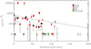 |
Fig. 10 Density of the HII regions as a function of the distance to the galaxy nucleus. The dotted line represents the fit of Eq. (7) to the data, excluding the upper limits. Symbols are the same as in Fig. 9. |
 |
Fig. 11 Diagnostic diagram to show the excitation properties of the detected HII regions. The red solid line represents the theoretical upper boundaries for HII regions from Dopita et al. (2000). Symbols are the same as in Fig. 9. |
 |
Fig. 12 NGC 1232B galaxy spectrum. Red and blue dotted lines mark the main emission lines detected. Orange dotted lines mark artificial effects due to instrumental problems. |
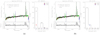 |
Fig. 13 Stellar population spectral fitting of the galaxy NGC 1232B. (a) and (b): spectrum fitted with BC03 and V15 models, respectively. In each figure, top-left panel: observed spectrum in black and the fitted synthetic spectrum in red. Bottom-left panel: residual of the difference between the two. Right panel: SFH, which indicates the contribution of each population age and metallicity to the final synthetic spectrum. |
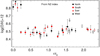 |
Fig. 14 Oxygen radial abundance gradient obtained from the N2 index. Distances are normalised to the disc effective radius. Symbols are the same as in Fig. 9. |
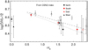 |
Fig. 15 Oxygen radial abundance gradient obtained from the O3N2 index. Distances are normalised to the disc effective radius. The dotted line represents the fit to the distribution with r∕re > 0.5. The dashed line is the same fit, including the data from Bresolin et al. (2005). Symbols are the same as in Fig. 9. |
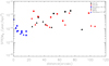 |
Fig. 16 SFR as a function of the distance to the nucleus of NGC 1232. |
7 SFR distribution
The SFR is an important factor in the chemical evolution of a galaxy. Its value gives the total amount of gas converted into stars over a given time interval, which may depend on several environmental properties. The SFR is related to the Hα luminosity, as defined by Calzetti et al. (2007):
 (15)
(15)
The SFR for each HII region is presented in Fig. 16 and also in Table 6. As found by de Souza et al. (2018), the central region of the galaxy has a lower SFR than the most remote regions. For the slit positions of this work, the N-S regions seem to have higher star formation compared to the E-W direction for the outter regions. On average, the values obtained for SFR in this study are in agreement with the values of de Souza et al. (2018).
8 Discussion and conclusions
In this work, we study the galaxy NGC 1232 with long-slit spectroscopy at two different, perpendicular positions. NGC 1232 is a nearby spiral galaxy, practically face-on, which makes it an ideal laboratory for the study of star formation. Recent X-ray studies have suggested that it recently collided with a dwarf galaxy (Garmire 2013), of which there is no apparent remnant. The effects of such a collision might have been a localised increase in star formation in the galaxy, as suggested by the results of de Souza et al. (2018).
From the Hα emission peaks along the slits positioned in the N-S and E-W directions, we extracted the HII regions analysed in this work. Before measuring the emission lines, we fit the underlying stellar population of the galaxy using the spectral fitting technique. We found that both the N-S and E-W directions present a stellar population gradient typical of spiral galaxies, with the fraction of the young component increasing progressively when moving outwards from the center. Conversely, the old component becomes less important out of the galaxy nucleus. The E-W direction seems to have a younger population in the nucleus compared to the N-S direction. We believe that this is both connected with the slit position (the N-S slit is positioned slightly to the west of the nucleus) and the presence of a small bar in the E-W direction.
After the subtraction of the stellar population, we measured the emission lines in each HII region. For many of them, it was only possible to measure Hα and [NII] lines but when possible, we determined the extinction coefficient and corrected the lines for it. These lines were used to determine the electron density profile of the galaxy and the oxygen abundance gradient.
The existence of a radially decreasing abundance gradient in spiral galaxies has been well-established by several observations over the years (Searle 1971; Martin & Roy 1992; Zaritsky et al. 1994; van Zee et al. 1998; Martins & Viegas 2000; Kennicutt et al. 2003; Bresolin et al. 2012; Sánchez et al. 2014; Sánchez-Menguiano et al. 2016a; Kaplan et al. 2016; Belfiore et al. 2017; Poetrodjojo et al. 2019; Kreckel et al. 2019), which support the inside-out disk scenario. However, deviations from a simple linear decrease have been reported in recent years, with a flattening or drop of the relation in the central regions and sometimes aflattening of the curve in the outer parts (Belley & Roy 1992; Martin & Roy 1995; Vilchez & Esteban 1996; Roy & Walsh 1997; Sánchez-Menguiano et al. 2018). Even the purely radial picture has been questioned of late (Kreckel et al. 2019) since spiral arms, bars, and stellar feedback drive mixing and gas flows, affecting the gas-phase abundances azimuthally (Grand et al. 2016; Sánchez-Menguiano et al. 2016b; Ho et al. 2017; Yang & Krumholz 2012; Petit et al. 2015; de Avillez & Mac Low 2002; Krumholz & Ting 2018). This is a difficult effect to measure because a large number of objects per galaxy are needed to detect it. Evidence has been found to support it (Kreckel et al. 2019) but it is, nonetheless, still inconclusive. Aside from that, there is the complication of defining the real boundary of the HII regions and, in many instances, the surrounding diffuse ionised gas (DIG) contaminates the observed spectrum of these objects (Poetrodjojo et al. 2019). This contamination might cause a flattening of the metallicity gradient.
With our data, it is difficult to fully characterise the abundance gradient of NGC 1232 due to the weaknesses of some important lines for the diagnostics and the small number of objects detected. We were able to determine two abundance indexes from our data, N2 and O3 N2. Despite having more measurements for the N2, this index is known to be less sensible to higher abundances, which hampers its efficacy to characterise the galaxy’s gradient. From the few determinations we have of O3 N2, we were able to measure an oxygen abundance gradient of −0.16 dex/r − e, which is within the expected value for a spiral galaxy. We also believe there might be an abundance drop towards the center, although it is not possible to determine where the drop begins. Many different mechanisms have been proposed in the literature to explain the deviation from the negative gradient in spiral galaxies, such as satellite accretion (Qu et al. 2015; Bird et al. 2012). It would be tempting to assume that the broken gradient profile found for NGC 1232 could be an extra evidence of the collision seen in X-ray, but recent observational works have found no dependence of the presence of the broken profile with either environment, morphological type, or the presence of bars (Sánchez-Menguiano et al. 2018).
For all the characteristics studied in this paper (electron density profile, stellar populations, SFR distribution, and abundance gradients), we found no deviation from a typical spiral galaxy and only tenuous differences between some of the directions. Therefore, through our long-slit analysis, we found no clear evidence of the collision seen in X-ray. We believe that if the collision caused a disturbance in the galaxy, it will be a small disturbance not clearly observed in a small number of objects. A final understanding of the effect or not of this possible collision can only be achieved with a deep spectroscopic observation covering the whole galaxy (maybe with an IFU observation).
The northernmost Hα emission peak measured in the N-S slit was not an HII region of NGC 1232, but a background galaxy, named by Arp (1982) as NGC 1232B. To the best of our knowledge, we provide the first characterisation of that galaxy so far in the literature. We derived a redshift of z = 0.09261 using the emission lines detected on its spectrum. Moreover, by means of the stellar population analysis, Baldwin, Phillips & Terlevich (BPT) diagrams, and emission line criteria by Bergvall et al. (2016), we classified NGC 1232B as a starburst galaxy.
Acknowledgements
We thank the referee for the valuable comments that greatly improved the paper. Based on observations obtained at the Southern Astrophysical Research (SOAR) telescope, which is a joint project of the Ministério da Ciência, Tecnologia, e Inovação (MCTI) da República Federativa do Brasil, the US National Optical Astronomy Observatory(NOAO), the University of North Carolina at Chapel Hill (UNC), and Michigan State University (MSU). F.L.C. acknowledges CAPES for financial support. L.M. thanks CNPQ for financial support through grant 306359/2018-9 and FAPESP through grant 2015/14575-0. A.R.A. thanks CNPq for partial support to this work.
Appendix A Stellar population spectral fitting for all apertures of NGC 1232
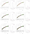 |
Fig. A.1 Stellar-population spectral fitting of the HII regions of NGC 1232, a apertures 02, 03, and 04 of the N-S slit. Left figures: spectra fitted with BC03 and right: with V15 models. In each figure, top left panel: observed spectrum in black, and the fitted synthetic spectrum in red. Bottom left panel: residual of the difference between the two. Right panel: star formation history (SFH), which indicates the contribution of each population age and metallicity to the final synthetic spectrum. |
References
- Alloin, D., Collin-Souffrin, S., Joly, M., & Vigroux, L. 1979, A&A, 78, 200 [Google Scholar]
- Arp, H. 1982, ApJ, 263, 54 [NASA ADS] [CrossRef] [Google Scholar]
- Asari, N. V., Cid Fernandes, R., Stasińska, G., et al. 2007, MNRAS, 381, 263 [NASA ADS] [CrossRef] [MathSciNet] [Google Scholar]
- Belfiore, F., Maiolino, R., Tremonti, C., et al. 2017, MNRAS, 469, 151 [NASA ADS] [CrossRef] [Google Scholar]
- Belley, J., & Roy, J.-R. 1992, ApJS, 78, 61 [NASA ADS] [CrossRef] [Google Scholar]
- Bergvall, N., Marquart, T., Way, M. J., et al. 2016, A&A, 587, A72 [NASA ADS] [CrossRef] [EDP Sciences] [Google Scholar]
- Bird, J. C., Kazantzidis, S., & Weinberg, D. H. 2012, MNRAS, 420, 913 [NASA ADS] [CrossRef] [Google Scholar]
- Boissier, S., & Prantzos, N. 1999, MNRAS, 307, 857 [NASA ADS] [CrossRef] [Google Scholar]
- Bresolin, F., Schaerer, D., Delgado, R. G., & Stasińska, G. 2005, A&A, 441, 981 [NASA ADS] [CrossRef] [EDP Sciences] [Google Scholar]
- Bresolin, F., Kennicutt, R. C., & Ryan-Weber, E. 2012, ApJ, 750, 122 [NASA ADS] [CrossRef] [Google Scholar]
- Brinchmann, J., Charlot, S., White, S. D. M., et al. 2004, MNRAS, 351, 1151 [NASA ADS] [CrossRef] [Google Scholar]
- Bruzual, G., & Charlot, S. 2003, MNRAS, 344, 1000 [NASA ADS] [CrossRef] [Google Scholar]
- Calzetti, D., Kennicutt, R. C., Engelbracht, C. W., et al. 2007, ApJ, 666, 870 [NASA ADS] [CrossRef] [Google Scholar]
- Cardelli, J. A., Clayton, G. C., & Mathis, J. S. 1989, ApJ, 345, 245 [NASA ADS] [CrossRef] [Google Scholar]
- Chiappini, C., Matteucci, F., & Romano, D. 2001, ApJ, 554, 1044 [NASA ADS] [CrossRef] [Google Scholar]
- Cid Fernandes, R., González Delgado, R. M., Schmitt, H., et al. 2004, ApJ, 605, 105 [NASA ADS] [CrossRef] [Google Scholar]
- Cid Fernandes, R., Mateus, A., Sodré, L., Stasińska, G., & Gomes, J. M. 2005a, MNRAS, 358, 363 [NASA ADS] [CrossRef] [Google Scholar]
- Cid Fernandes, R., González Delgado, R., Storchi-Bergmann, T., Martins, L. P., & Schmitt, H. 2005b, MNRAS, 356, 270 [NASA ADS] [CrossRef] [Google Scholar]
- de Avillez, M. A., & Mac Low, M.-M. 2002, ApJ, 581, 1047 [NASA ADS] [CrossRef] [Google Scholar]
- Denicoló, G., Terlevich, R., & Terlevich, E. 2002, MNRAS, 330, 69 [NASA ADS] [CrossRef] [Google Scholar]
- de Souza, A., Martins, L. P., Rodríguez-Ardila, A., & Fraga, L. 2018, AJ, 155, 234 [CrossRef] [Google Scholar]
- Díaz, A. I., & Pérez-Montero, E. 2000, MNRAS, 312, 130 [NASA ADS] [CrossRef] [Google Scholar]
- Dinerstein, H. L. 1990, in The Interstellar Medium in Galaxies (Berlin: Springer), 257 [CrossRef] [Google Scholar]
- Dopita, M. A. 1985, ApJ, 295, L5 [NASA ADS] [CrossRef] [Google Scholar]
- Dopita, M. A., & Ryder, S. D. 1994, ApJ, 430, 163 [NASA ADS] [CrossRef] [Google Scholar]
- Dopita, M., Kewley, L., Heisler, C., & Sutherland, R. 2000, ApJ, 542, 224 [NASA ADS] [CrossRef] [Google Scholar]
- Edmunds, M. G., & Greenhow, R. M. 1995, MNRAS, 272, 241 [NASA ADS] [CrossRef] [Google Scholar]
- Ferland, G. J., Porter, R. L., van Hoof, P. A. M., et al. 2013, Rev. Mex. Astron. Astrofis., 49, 137 [Google Scholar]
- Freeman, K. C. 1970, ApJ, 160, 811 [Google Scholar]
- Fu, J., Hou, J. L., Yin, J., & Chang, R. X. 2009, ApJ, 696, 668 [NASA ADS] [CrossRef] [Google Scholar]
- Garmire, G. P. 2013, ApJ, 770, 17 [CrossRef] [Google Scholar]
- Grand, R. J. J., Springel, V., Kawata, D., et al. 2016, MNRAS, 460, L94 [NASA ADS] [CrossRef] [Google Scholar]
- Gutiérrez, L., & Beckman, J. E. 2010, ApJ, 710, L44 [NASA ADS] [CrossRef] [Google Scholar]
- Ho, I. T., Seibert, M., Meidt, S. E., et al. 2017, ApJ, 846, 39 [NASA ADS] [CrossRef] [Google Scholar]
- Kaplan, K. F., Jogee, S., Kewley, L., et al. 2016, MNRAS, 462, 1642 [NASA ADS] [CrossRef] [Google Scholar]
- Kennicutt, Jr. R. C. 1989, ApJ, 344, 685 [NASA ADS] [CrossRef] [Google Scholar]
- Kennicutt, Jr R. C., Armus, L., Bendo, G., et al. 2003, PASP, 115, 928 [NASA ADS] [CrossRef] [Google Scholar]
- Kobulnicky, H. A., & Kewley, L. J. 2004, ApJ, 617, 240 [NASA ADS] [CrossRef] [Google Scholar]
- Koeppen, J. 1994, A&A, 281, 26 [Google Scholar]
- Kreckel, K., Ho, I. T., Blanc, G. A., et al. 2019, ApJ, 887, 80 [NASA ADS] [CrossRef] [Google Scholar]
- Krumholz, M. R., & Ting, Y.-S. 2018, MNRAS, 475, 2236 [CrossRef] [Google Scholar]
- Kuzio de Naray, R., McGaugh, S. S., & de Blok, W. J. G. 2004, MNRAS, 355, 887 [NASA ADS] [CrossRef] [Google Scholar]
- Lacey, C. G., & Fall, S. M. 1985, ApJ, 290, 154 [NASA ADS] [CrossRef] [Google Scholar]
- Mac Low, M.-M., & Ferrara, A. 1999, ApJ, 513, 142 [NASA ADS] [CrossRef] [Google Scholar]
- Marino, R. A., Rosales-Ortega, F. F., Sánchez, S. F., et al. 2013, A&A, 559, A114 [NASA ADS] [CrossRef] [EDP Sciences] [Google Scholar]
- Martin, P., & Roy, J.-R. 1992, ApJ, 397, 463 [NASA ADS] [CrossRef] [Google Scholar]
- Martin, P., & Roy, J.-R. 1995, ApJ, 445, 161 [NASA ADS] [CrossRef] [Google Scholar]
- Martins, L. P., & Viegas, S. M. M. 2000, A&A, 361, 1121 [NASA ADS] [Google Scholar]
- Martins, L. P., Rodríguez-Ardila, A., Diniz, S., Gruenwald, R., & de Souza, R. 2013, MNRAS, 431, 1823 [NASA ADS] [CrossRef] [Google Scholar]
- Mateus, A., Sodré, L., Cid Fernandes, R., et al. 2006, MNRAS, 370, 721 [NASA ADS] [CrossRef] [Google Scholar]
- Mathis, J. S. 1985, BAAS, 17, 596 [Google Scholar]
- Matteucci, F., & Francois, P. 1989, MNRAS, 239, 885 [NASA ADS] [CrossRef] [Google Scholar]
- McCall, M. L., Rybski, P. M., & Shields, G. A. 1985, ApJS, 57, 1 [NASA ADS] [CrossRef] [Google Scholar]
- Mollá, M., & Díaz, A. I. 2005, MNRAS, 358, 521 [NASA ADS] [CrossRef] [Google Scholar]
- Molla, M., Ferrini, F., & Diaz, A. I. 1996, ApJ, 466, 668 [NASA ADS] [CrossRef] [Google Scholar]
- Mollá, M., Ferrini, F., & Díaz, A. I. 1997, ApJ, 475, 519 [NASA ADS] [CrossRef] [Google Scholar]
- Osterbrock, D. E., & Ferland, G. J. 2006, Astrophysics Of Gas Nebulae and Active Galactic Nuclei (Mill Valley, CA: University science books) [Google Scholar]
- Pagel, B. E. J., Edmunds, M. G., Blackwell, D. E., Chun, M. S., & Smith, G. 1979, MNRAS, 189, 95 [NASA ADS] [CrossRef] [Google Scholar]
- Petit, A. C., Krumholz, M. R., Goldbaum, N. J., & Forbes, J. C. 2015, MNRAS, 449, 2588 [NASA ADS] [CrossRef] [Google Scholar]
- Pettini, M., & Pagel, B. E. J. 2004, MNRAS, 348, L59 [NASA ADS] [CrossRef] [Google Scholar]
- Pilkington, K., Few, C. G., Gibson, B. K., et al. 2012, A&A, 540, A56 [NASA ADS] [CrossRef] [EDP Sciences] [Google Scholar]
- Poetrodjojo, H., Groves, B., Kewley, L. J., et al. 2018, MNRAS, 479, 5235 [NASA ADS] [CrossRef] [Google Scholar]
- Poetrodjojo, H., D’Agostino, J. J., Groves, B., et al. 2019, MNRAS, 487, 79 [NASA ADS] [CrossRef] [Google Scholar]
- Prantzos, N., & Aubert, O. 1995, A&A, 302, 69 [NASA ADS] [Google Scholar]
- Prantzos, N., & Boissier, S. 2000, MNRAS, 313, 338 [NASA ADS] [CrossRef] [Google Scholar]
- Proxauf, B., Öttl, S., & Kimeswenger, S. 2014, A&A, 561, A10 [NASA ADS] [CrossRef] [EDP Sciences] [Google Scholar]
- Qu, Z., Li, Z., Chen, Y., et al. 2015, PASP, 127, 211 [CrossRef] [Google Scholar]
- Roy, J. R., & Walsh, J. R. 1997, MNRAS, 288, 715 [NASA ADS] [CrossRef] [Google Scholar]
- Sánchez, S. F. 2020, ARA&A, 58 [CrossRef] [Google Scholar]
- Sánchez, S. F., Rosales-Ortega, F. F., Marino, R. A., et al. 2012, A&A, 546, A2 [NASA ADS] [CrossRef] [EDP Sciences] [Google Scholar]
- Sánchez, S. F., Rosales-Ortega, F. F., Iglesias-Páramo, J., et al. 2014, A&A, 563, A49 [NASA ADS] [CrossRef] [EDP Sciences] [Google Scholar]
- Sánchez-Blázquez, P., Rosales-Ortega, F. F., Méndez-Abreu, J., et al. 2014, A&A, 570, A6 [NASA ADS] [CrossRef] [EDP Sciences] [Google Scholar]
- Sánchez-Menguiano, L., Sánchez, S., Kawata, D., et al. 2016a, ApJ, 830, L40 [NASA ADS] [CrossRef] [Google Scholar]
- Sánchez-Menguiano, L., Sánchez, S. F., Pérez, I., et al. 2016b, A&A, 587, A70 [NASA ADS] [CrossRef] [EDP Sciences] [Google Scholar]
- Sánchez-Menguiano, L., Sánchez, S. F., Pérez, I., et al. 2018, A&A, 609, A119 [NASA ADS] [CrossRef] [EDP Sciences] [Google Scholar]
- Sanders, R. L., Shapley, A. E., Reddy, N. A., et al. 2020, MNRAS, 491, 1427 [CrossRef] [Google Scholar]
- Schmidt, M. 1959, ApJ, 129, 243 [NASA ADS] [CrossRef] [Google Scholar]
- Searle, L. 1971, ApJ, 168, 327 [NASA ADS] [CrossRef] [Google Scholar]
- Shapley, A. E., Erb, D. K., Pettini, M., Steidel, C. C., & Adelberger, K. L. 2004, ApJ, 612, 108 [NASA ADS] [CrossRef] [Google Scholar]
- Tilanus, R. P. J., & Allen, R. J. 1991, A&A, 244, 8 [NASA ADS] [Google Scholar]
- Tsujimoto, T., Yoshii, Y., Nomoto, K., & Shigeyama, T. 1995, A&A, 302, 704 [NASA ADS] [Google Scholar]
- van Zee, L., & Bryant, J. 1999, AJ, 118, 2172 [NASA ADS] [CrossRef] [Google Scholar]
- van Zee, L., Salzer, J. J., Haynes, M. P., O’Donoghue, A. A., & Balonek, T. J. 1998, AJ, 116, 2805 [NASA ADS] [CrossRef] [Google Scholar]
- Vazdekis, A., Coelho, P., Cassisi, S., et al. 2015, MNRAS, 449, 1177 [NASA ADS] [CrossRef] [Google Scholar]
- Vilchez, J. M., & Esteban, C. 1996, MNRAS, 280, 720 [NASA ADS] [CrossRef] [Google Scholar]
- Wyse, R. F. G., & Silk, J. 1989, ApJ, 339, 700 [NASA ADS] [CrossRef] [Google Scholar]
- Yang, C.-C., & Krumholz, M. 2012, ApJ, 758, 48 [NASA ADS] [CrossRef] [Google Scholar]
- Zaritsky, D., Kennicutt, Robert C., J., & Huchra, J. P. 1994, ApJ, 420, 87 [NASA ADS] [CrossRef] [Google Scholar]
Distance from NED (NASA/IPAC Extragalactic Database).
Redshifts obtained from NED (NASA/IPAC Extragalactic Database).
IRAF is distributed and maintained by National Optical Astronomy (NOAO), which are operated by the Association of Universities for Research in Astronomy, Inc., under a cooperative agreement with the National Science Foundation.
All Tables
Results of the stellar population fitting for the HII regions of the N-S slit and NGC 1232B.
Emission line fluxes for the N-S and E-W apertures of NGC 1232 and for NGC 1232B.
Reddening corrected emission line fluxes (relative to Hβ) for the N-S and E-W slits.
All Figures
|
Fig. 1 (a) Hα image of NGC 1232 from de Souza et al. (2018). The white lines represent the slits from where the HII regions were extracted along the N-S and E-W directions. (b) Spatial distribution of flux in Hα of the slits N-S (top) and E-W (bottom), showing the peaks which correspond to each HII region (and NGC 1232B) extracted. The numbers on top correspond to their names in Table 1 and the size of the extraction of each HII regions is shown by the ranges below these numbers. |
| In the text | |
|
Fig. 2 Spectra of HII regions from the N-S slit. The dotted lines in red and blue mark the main emission lines detected. Dotted orange lines mark artificial effects due to to instrumental problems. The numbers on the right side of the plot identify the apertures. |
| In the text | |
|
Fig. 3 Spectra of HII regions from the E-W slit. The dotted lines in red and blue mark the main emission lines detected. Dotted orange lines mark artificial effects due to instrumental problems. The numbers to the right side of the plot identify the apertures. |
| In the text | |
|
Fig. 4 Example of the stellar population spectral fitting. (a) and (c): aperture 01 (nucleus of the galaxy, N-S slit) fitted with BC03 and V15 models, respectively, and (b) and (d): aperture 13(N-S slit), also fitted with BC03 and V15 models, respectively. In each figure, top left panel: observed spectrum inblack, and the fitted synthetic spectrum in red. The regions marked in green represent masked intervals, ignored by STARLIGHT because of the presence of emission lines. Bottom left panel: residual of the difference between the two. Right panel: star formation history (SFH), which means the contribution of each population age and metallicity to the final synthetic spectrum. |
| In the text | |
|
Fig. 5 Stellar population gradient for the N-S slit of NGC 1232, obtained with BC03 models (a) and V15 models (b). Triangles represent the southern region and circles the northern region. |
| In the text | |
|
Fig. 6 Stellar population gradient for the E-W slit of NGC 1232, obtained with BC03 models (a) and V15 models (b). Triangles represent the western region and circles the eastern region. |
| In the text | |
|
Fig. 7 Extinction coefficient as a function of distance to the nucleus of the galaxy NGC 1232, for the N-S (a) and E-W (b) slit. Open symbols in both figures are the HII regions from Bresolin et al. (2005). |
| In the text | |
|
Fig. 8 Comparison of reddening-corrected line intensities (in units of Hβ = 100), of the most common lines, measured in the current work (horizontal axis) and values from the literature (vertical axis). Red points refer to [OIII]λ5007, blue points to [NII]λ6583 and green points to [SII]λ6716 and [SII]λ6731. |
| In the text | |
|
Fig. 9 Density-sensitive diagnostic diagram using the line ratio [SII]λ6716/[SII]λ6731 as a function of the distance to the galaxy nucleus. Open symbols are data from Bresolin et al. (2005). Colors and symbols are the same as for our data, and open gray squares are the HII regions that are in a different direction than the ones covered by our slits. |
| In the text | |
|
Fig. 10 Density of the HII regions as a function of the distance to the galaxy nucleus. The dotted line represents the fit of Eq. (7) to the data, excluding the upper limits. Symbols are the same as in Fig. 9. |
| In the text | |
|
Fig. 11 Diagnostic diagram to show the excitation properties of the detected HII regions. The red solid line represents the theoretical upper boundaries for HII regions from Dopita et al. (2000). Symbols are the same as in Fig. 9. |
| In the text | |
|
Fig. 12 NGC 1232B galaxy spectrum. Red and blue dotted lines mark the main emission lines detected. Orange dotted lines mark artificial effects due to instrumental problems. |
| In the text | |
|
Fig. 13 Stellar population spectral fitting of the galaxy NGC 1232B. (a) and (b): spectrum fitted with BC03 and V15 models, respectively. In each figure, top-left panel: observed spectrum in black and the fitted synthetic spectrum in red. Bottom-left panel: residual of the difference between the two. Right panel: SFH, which indicates the contribution of each population age and metallicity to the final synthetic spectrum. |
| In the text | |
|
Fig. 14 Oxygen radial abundance gradient obtained from the N2 index. Distances are normalised to the disc effective radius. Symbols are the same as in Fig. 9. |
| In the text | |
|
Fig. 15 Oxygen radial abundance gradient obtained from the O3N2 index. Distances are normalised to the disc effective radius. The dotted line represents the fit to the distribution with r∕re > 0.5. The dashed line is the same fit, including the data from Bresolin et al. (2005). Symbols are the same as in Fig. 9. |
| In the text | |
|
Fig. 16 SFR as a function of the distance to the nucleus of NGC 1232. |
| In the text | |
|
Fig. A.1 Stellar-population spectral fitting of the HII regions of NGC 1232, a apertures 02, 03, and 04 of the N-S slit. Left figures: spectra fitted with BC03 and right: with V15 models. In each figure, top left panel: observed spectrum in black, and the fitted synthetic spectrum in red. Bottom left panel: residual of the difference between the two. Right panel: star formation history (SFH), which indicates the contribution of each population age and metallicity to the final synthetic spectrum. |
| In the text | |
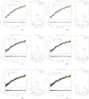 |
Fig. A.2 Same as Fig. A.1 but for apertures 05, 06, and 07 of the N-S slit. |
| In the text | |
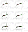 |
Fig. A.3 Same as Fig. A.1 but for apertures 08, 09, and 10 of the N-S slit. |
| In the text | |
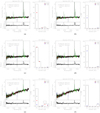 |
Fig. A.4 Same as Fig. A.1 but for apertures 11, 12, and 14 of the N-S slit. |
| In the text | |
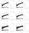 |
Fig. A.5 Same as Fig. A.1 but for apertures 15, 16, and 17 of the N-S slit. |
| In the text | |
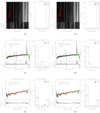 |
Fig. A.6 Same as Fig. A.1 but for apertures 18 and 19 of N-S slit and aperture 01 of E-W slit. |
| In the text | |
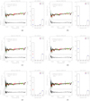 |
Fig. A.7 Same as Fig. A.1 but for apertures 02, 03, and 04 of E-W slit. |
| In the text | |
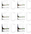 |
Fig. A.8 Same as Fig. A.1 but for apertures 05, 06, and 07 of the E-W slit. |
| In the text | |
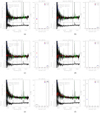 |
Fig. A.9 Same as Fig. A.1 but for apertures 08, 09, and 10 of the E-W slit. |
| In the text | |
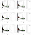 |
Fig. A.10 Same as Fig. A.1 but for apertures 11, 12, and 13 of the E-W slit. |
| In the text | |
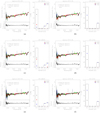 |
Fig. A.11 Same as Fig. A.1 but for apertures 14, 15, and 16 of the E-W slit. |
| In the text | |
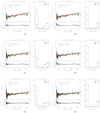 |
Fig. A.12 Same as Fig. A.1 but for apertures 17, 18, and 19 of the E-W slit. |
| In the text | |
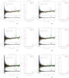 |
Fig. A.13 Same as Fig. A.1 but for apertures 20, 21, and 22 of the E-W slit. |
| In the text | |
Current usage metrics show cumulative count of Article Views (full-text article views including HTML views, PDF and ePub downloads, according to the available data) and Abstracts Views on Vision4Press platform.
Data correspond to usage on the plateform after 2015. The current usage metrics is available 48-96 hours after online publication and is updated daily on week days.
Initial download of the metrics may take a while.