| Issue |
A&A
Volume 642, October 2020
|
|
|---|---|---|
| Article Number | A152 | |
| Number of page(s) | 13 | |
| Section | Interstellar and circumstellar matter | |
| DOI | https://doi.org/10.1051/0004-6361/202037946 | |
| Published online | 13 October 2020 | |
VLTI/PIONIER reveals the close environment of the evolved system HD 101584★,★★
1
Instituut voor Sterrenkunde (IvS), KU Leuven, Celestijnenlaan 200D,
3001
Leuven,
Belgium
e-mail: This email address is being protected from spambots. You need JavaScript enabled to view it.
2
Department of Space, Earth and Environment, Chalmers University of Technology, Onsala Space Observatory,
43992
Onsala, Sweden
3
ESO,
Karl-Schwarzschild-Str. 2,
85748,
Garching bei München Germany
4
ESO,
Alonso de Cordova 3107,
Vitacura,
Santiago, Chile
5
Department of Physics and Astronomy, Uppsala University,
Box 516,
75120
Uppsala, Sweden
6
National Astronomical Observatory of Japan,
2-21-1 Osawa,
Mitaka,
Tokyo
181-8588, Japan
Received:
12
March
2020
Accepted:
25
August
2020
Abstract
Context. The observed orbital characteristics of post-asymptotic giant branch and post-red giant branch (post-RGB) binaries are not understood. We suspect that the missing ingredients needed to explain them probably lie in the continuous interaction of the central binary with its circumstellar environment.
Aims. We aim at studying the circumbinary material in these complex systems by investigating the connection between the innermost structures and large-scale structures.
Methods. We perform high-angular resolution observations of HD 101584 in the near-infrared continuum. HD 101584 has a complex structure as seen at millimeter wavelengths, with a disk-like morphology and a bipolar outflow due to an episode of a strong binary interaction. To account for the complexity of the target, we first perform an image reconstruction and use this result to fit a geometrical model to extract the morphological and thermal features of the environment.
Results. The image reveals an unexpected double ring structure. We interpret the inner ring as having been produced by emission from dust located in the plane of the disk, and the outer ring having been produced by emission from dust that is located 1.6 [D/1kpc] au above the disk plane. The inner ring diameter (3.94 [D/1kpc] au) and temperature (T = 1540 ± 10 K) are compatible with the dust sublimation front of the disk. The origin of the out-of-plane ring (with a diameter of 7.39 [D/1kpc] au and a temperature of 1014 ± 10 K) could be episodic ejection or a dust condensation front in the outflow.
Conclusions. The observed outer ring is possibly linked with the blue-shifted side of the large-scale outflow seen by the Atacama Large Millimeter/submillimeter Array and may trace its launching location to the central star. Such observations place morphological constraints on the ejection mechanism. Additional observations are needed to constrain the origin of the out-of-plane structure.
Key words: stars: AGB and post-AGB / binaries: general / circumstellar matter / stars: winds, outflows / techniques: high angular resolution / techniques: interferometric
The reconstructed images are only available at the CDS via anonymous ftp to cdsarc.u-strasbg.fr (130.79.128.5) or via http://cdsarc.u-strasbg.fr/viz-bin/cat/J/A+A/642/A152
Based on observations collected at the European Organisation for Astronomical Research in the Southern Hemisphere under ESO programme 099.D-0088.
© ESO 2020
1 Introduction
Binarity is frequent in stars and can strongly impact their evolution (Duchêne & Kraus 2013; Sana et al. 2014). When the separation on the main sequence is on the order of an astronomical unit, binary interaction will severely impact the stellar evolution when the radius of the star increases, giving rise to various types of objects and phenomena (such as barium stars, asymmetric planetary nebulae, and supernovae type Ia). In this paper, we focus on low- and intermediate-mass stars with main sequence masses between about 0.8 and 8 M⊙. The stellar radius increases dramatically during the red giant and asymptotic giant phases, and, depending on the binary separation, this will lead to strong interaction via tides, wind-Roche lobe overflow (e.g., Abate et al. 2013), or full Roche lobe overflow (e.g., Ivanova et al. 2013). Their stellar evolution is, hence, different than that for single stars. Single stars eject their envelope in an episode of strong winds at the end of the asymptotic giant branch (AGB) phase and become contracting white dwarfs, possibly giving rise to planetary nebulae. In the case of the presence of a close companion, the common-envelope evolution leads to envelope ejection, terminating the AGB phase or even the red giant branch (RGB) phase (Kamath et al. 2015, 2016; Kamath & Van Winckel 2019). Those objects are referred to as post-AGB or post-RGB binaries (Van Winckel 2003).
While the dust envelope surrounding the red giant star and its intrinsic variability limit our ability to detect a companion, once the envelope is ejected (in the post-AGB or post-RGB phase; Van Winckel 2003, 2018), binarity can be detected by radial velocity monitoring. We can therefore observe products of the strong binary interaction phase, such as the resulting orbits and the properties of the circumbinary environment. A disk-like infrared excess in the spectral energy distribution (SED) is strongly correlated with the presence of a binary system (Van Winckel 2018).
Spatially resolved observations of those circumbinary environments reveal their high degree of complexity (Hillen et al. 2014, 2015; Kluska et al. 2018, 2019). Only intensive observing campaigns dedicated to imaging can uncover it (Hillen et al. 2016). The picture that emerges of these systems, based mainly on infrared interferometric imaging of IRAS 08544-4431 (Hillen et al. 2016), consists of a post-AGB star, a secondary with a circumsecondary accretion disk and a jet, a circumbinary disk perturbed by the inner binary, and extended emission of unknown origin (disk, wind, or jet?). This picture needs to be confirmed with additional observations of other targets.
In this paper, we present near-infrared interferometric observations of the evolved object HD 101584. The main star’s effective temperature was estimated to be around 8500 K (Sivarani et al. 1999; Kipper 2005). The binarity of HD 101584 was inferred from photometric and spectroscopic variations (Balmer jump, He I, and C II) with a period of 218 ± 0.7days (Bakker et al. 1996). However, a period of 144 days was also claimed from spectroscopic observations (Díaz et al. 2007). Hence, there exists considerable uncertainty regarding the binary characteristics, even to the extent that the existence of a present companion can be discussed. However, the large-scale structure of the circumstellar environment seen in the Atacama Large Millimeter/submillimeter Array (ALMA) data (see below) strongly suggests that HD 101584 was a binary that went through a common-envelope process. Whether this ended before or by a merger plays no role in the interpretation in this paper, and we will therefore refer to the source as the HD 101584 system. In Sect. 5.4, we will discuss the implication of our observations on the possible present binary nature of HD 101584.
The Gaia parallax of HD 101584, 0.48 ± 0.04 mas, is on the order of the possible binary separation (as derived in Sect. 5.4). Therefore, the distance estimate may be biased by the orbital movement of the primary. Following Olofsson et al. (2019), we give the distance-dependent results as their values at 1 kpc, as well as their scaling with distance. Despite the lack of a reliable distance to HD 101584, the evolutionarystatus of this system was determined to be, most likely, a post-RGB binary (Olofsson et al. 2019). Its low 12CO/13CO ratio, ~13, indicates that it is on or beyond the RGB. The 17O/18O ratio of 0.2 ± 0.08 points toward a low initial mass of the star (≲1.3 M⊙, assuming aninitial solar abundance ratio of 0.18; Karakas & Lattanzio 2014; De Nutte et al. 2017). The higher luminosity of a post-AGB star would require a larger distance to the system (that would actually match the Gaia parallax) than in the case of a post-RGB star. This would make the estimated initial mass (the present stellar mass plus the mass of the ejected gas) less consistent with the initial stellar mass estimated from the oxygen isotope ratios. Hence, a post-RGB evolutionary status is preferred.
This system was extensively studied with ALMA (Olofsson et al. 2015, 2017, 2019). The morphology of the stellar environment as traced by submm gas and dust emission can be separated into four components: the central compact source (CCS), the equatorial density enhancement (EDE), the high-velocity outflow (HVO), and the hourglass structure (HGS). The CCS has a full width of half maximum size smaller than 100 [D/1kpc] au1 and emits in both continuum and numerous molecular lines. It coincides in size with the mid-infrared emission detected by interferometry (Hillen et al. 2017). The most likely interpretation is that the CCS corresponds to the circumstellar disk. The EDE is seen mainly in molecular lines, is in slow expansion, and has an almost circular structure (with a diameter of ~2”). It is interpreted as an almost face-on disk-like (or torus-like) structure with a possible connection to the CCS. The HVO is elongated in the direction of PA ~ 90°. It extends to a projected distance of 4” from the CCS in both directions, reaching velocities of 150 km s−1. The blue-shifted side points toward the west. The HVO ends at extreme-velocity spots (at ±150 km s−1 with respect to the systemic velocity) seen on both sides of the CCS in many molecular lines. The HVO and the extreme-velocity spots reveal a slightly S-shaped morphology, possibly indicating jet precession. Finally, the HGS traced in CO(2–1) has a roughly elliptical morphology and surrounds the HVO. It is likely produced by pressure from the HVO toward its sides. There is also evidence for a secondary HGS that has a slightly different orientation, possibly tracing a previous outflow event.
It is interesting to note that nebulae with such extreme circumstellar characteristics are also seen around objects that are claimed to be stellar mergers. For example, CK Vul, which was recently observed by ALMA, has a similar bipolar nebula and high outflow velocities (~100 km s−1; Eyres et al. 2018). The nebula is associated with a luminous red nova (LRN) event that took place in 1670 (Shara et al. 1985). It is advocated that the cause of an LRN may either be a giant eruption or, more likely, a stellar merger (Pastorello et al. 2019). The latter was argued in the case of CK Vul (Kato 2003; Eyres et al. 2018). The luminosity of the central star of CK Vul is low, however, around 1 L⊙, and its infrared excess does not show a continuous disk-like excess SED characteristic as in the cases of HD 101584 and post-AGB binaries. Nevertheless, another target, the Boomerang Nebula, with a more luminous central star (around 100 L⊙) and a disk-like SED, also has a similar large-scale morphology. It was argued to be a post-AGB or post-RGB merger based on energy balance computations (Sahai et al. 2017).
In this paper, we present high-angular resolution observations in the near-infrared to uncover the structure of the inner environmentof HD 101584 and probe the launching region of the bipolar jet. We also aim to put additional constraints on the evolutionarystatus by resolving the inner binary and obtaining the angular separation. Because the object has a complex structure, we performed image reconstruction to retrieve the emission morphology without using a model. We first present the infrared interferometric observations (Sect. 2) and describe the image reconstruction (Sect. 3). Then we apply a geometrical model to retrieve geometrical and thermal information on the differentobserved components of the system (Sect. 4). Finally, we discuss our findings and interpret the observed morphology (Sect. 5) before presenting our conclusions (Sect. 6).
2 Observations
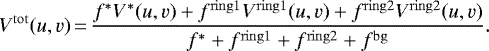
The observations were conducted using the Precision Integrated-Optics Near-infrared Imaging ExpeRiment (PIONIER) instrument (Le Bouquin et al. 2011) at the Very Large Telescope Interferometer (VLTI) between April 10, 2017, and May 20, 2017 (see Table A.1). PIONIER is a four-beam interferometric combiner in the near-infrared H-band (central wavelength of 1.65 μm). The H-band is covered with six wavelength channels (R ~ 40). This instrument provides two observables: the squared visibilities (V2), which are related to the size of the target, and closure phases (CPs), which are related to the degree of (non-)point symmetry. The data is plotted in Fig. 1 and is made of 297 V2 and 194 CP measurements. The (u, v)-plane is relatively well covered in every direction, covering scales from 1 to 21 mas (defined as λ∕2B, where λ is the observed wavelength and B is the baseline). From the V2 we can see that their level decreases sharply with spatial frequency (defined as the ratio between the baseline and the observational wavelength), meaning that the observed object is spatially resolved. At zero baseline, V2 reach unity. However, for the shortest baselines, V2 only reach the 0.8 level, suggesting the presence of over-resolved emission. The V2 do not reach zero at long baselines, meaning that part of the total flux is unresolved. The data is chromatic in such a way that V2 for short wavelengths are at higher levels than for long ones. It can be interpreted as the presence of a colder resolved component and an unresolved hot component, as seen in other targets with circumstellar material (e.g., protoplanetary disks around young stars; Kluska et al. 2014). Some CPs are significantly non-null, meaning that the source is not point symmetric.
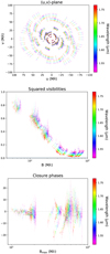 |
Fig. 1 VLTI/PIONIER dataset on HD 101584. Top: obtained (u, v)-coverage. Center: V2 against spatial frequency. Bottom: CP against the highest spatial frequency of a closure triangle. Spatial frequency is in log-scale. The color indicates the wavelength. |
3 Image reconstruction
To interpret the V2 and CP in a model-independent way, we used the technique of image reconstruction, as the (u, v)-coverage is good enough for an image to be reliably reconstructed. This technique enables determining the brightness distribution of the source model-independently to reveal any unpredicted morphologies. In this paper, we use the Multi-aperture Image Reconstruction Algorithm (MiRA) algorithm (Thiébaut 2008) together with the Semi-Parametric Approach to Reconstruct Chromatic Objects (SPARCO; Kluska et al. 2014). This approach allows one component of the target to be modeled and the other to be reconstructed by taking into account their temperature difference. For example, the star can be modeled as a point source, and its environment is reconstructed by taking into account the spectral index of each of the components. Given the angular scales probed by the (u, v)-coverage, our image is set to have 256 × 256 pixels with a pixel size of 0.15 mas. To reconstruct the image, the algorithm minimizes a cost function (f), defined from the Bayesian equation, that consists of two terms: f(x) = fdata(x) + μfrgl(x), where x is the image, fdata is the data likelihood term (here the χ2), frgl is the regularization term, and μ is the regularization weight. We used the quadratic smoothness regularization that is defined as: frgl = x − S.x, where S is a smoothing operator. This regularization was proven to be one of the best to be used in infrared interferometry (Renard et al. 2011) and is performing well in practice (e.g., Kluska et al. 2016; Hillen et al. 2016).
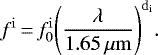
To reconstruct the image with the SPARCO approach, one needs to determine the regularization weight (μ) and the chromatic parameters, that is to say, the stellar-to-total flux ratio at 1.65 μm ( ) and the spectral index of the environment (denv). This process is described in detail in Kluska et al. (2016), but we recall the steps here: we chose μ and performed a grid on
  and denv to find the pair of these parameters that minimizes the cost function f (see Appendix B). For this object, the chromatic parameters are degenerate (see Fig. 2). We nevertheless chose the pair of chromatic parameters with the lower f to obtain the final image. However, in Sect. 4 we perform an image reconstruction with another pair of chromatic parameters constrained from our geometric model, showing the impact of different chromatic parameters on the image. Finally, to determine the significant structure in the image, we performed a bootstrap on the dataset. It consists in building a new dataset by drawing baselines for V2 and closure triangles for CPs until we reach the same number of data points. Each baseline or triangle can be drawn several or zero times. In order to find the optical regularization weight, we used the L-curve method as described in Kluska et al. (2016). For different regularization weights μ, we computed both the values of thelikelihood (fdata) and the regularization term (frgl) values. On a log–log plot, those values will trace two asymptotes for low and high values of the regularization weight, tracing the regimes where the likelihood and the regularization term dominate. Finally, we have chosen to use μ = 109, where the image is well regularized while still reproducing the data (we detail the impact of the regularization in Appendix C).
In Fig. 3, we can see the image reconstruction with the 5-σ significance contour. The image reconstruction reproduces the data well with a reduced  of 1.38 (see also Fig. D.1). The best pair of chromatic parameters are
  = 0.244 and denv = 2.45. This translates into a stellar-to-total flux ratio of 24.4% at 1.65 μm and an image spectral index of a black body having a temperature of ~1170 K, assuming a spectral index of d logFλ∕d logλ = −3.1 (as expected for a Teff ≃ 8500 K; Olofsson et al. 2019)for the central star. In the image (Fig. 3), there is a complex structure that appears to be two rings: the brightest one being close to the star and the fainter one being larger and probably slightly shifted with respect to the first one. The two rings are above 5-σ significance in the image. There are some small features that are marginally more significant than 5-σ, but, as theirexistence is not certain, we do not take them into account in this study.
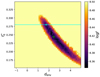 |
Fig. 2 Logarithm of the cost function f as a function of the chromatic parameters |


4 Geometrical modeling
Having established the morphological features present in the image (a hot point source and two colder rings), we want to obtain quantitative values describing the morphology and the relative emissions of the different components of the system. To achieve this, we performed geometrical model fitting. Inspired by the image reconstruction, we designed a geometrical model that is composed of a point sourceto model the central star, two rings, and a background for the over-resolved flux. The model is described in Appendix E and has 15 parameters. The central star is defined by three parameters: the stellar-to-total flux ratio ( ) and its coordinates relative to the centerof the inner ring (Δx and Δy). The rings are defined by: their diameters (rD1 and rD2 for the inner and outer rings, respectively); their full width at half maximum in units of the ring radius (rW1 and rW2, respectively); their ring-to-total flux ratios (
 and
and  ); and their black body temperatures (T1 and T2), constrained from the changing flux ratios between the components using all spectral channels. We assumed that one of the rings belongs to a disk called the midplane. The other ring could be in the same plane (and part of the same disk), or it could be located out of this plane and part of another structure, for example the HGS, as discussed below. We assumed their inclinations (i) and position angles (PAs) to be the same, but we allowed the outer ring to be shifted with respect to the inner ring in the direction of the minor-axis (ΔRring2). Finally, the background is defined by the background-to-total flux ratio (
 ) and its spectral index (dbg). Because the flux ratios are relative quantities, the ring1-to-total flux ratio is not fitted but deduced from the others as being
  = 1-
= 1- -
- -
- . In order to explore the parameters of such a complex model, we employed the two-step approach used and explained in Kluska et al. (2019). The geometrical model was transformed into V2 and CP values for each baseline of the original dataset. The fit was then performed in the Fourier domain. We started with a distribution of first guesses of the parameters based on the image reconstruction. We then explored the parameter space with a genetic algorithm (using Distributed Evolutionary Algorithms in Python framework; Fortin et al. 2012) that efficiently finds minima. Then, we used the best solutions from the previous step with the Markov chain Monte Carlo (MCMC) sampler emcee (Foreman-Mackey et al. 2013) to derive errors. The errors on several parameters are very small (Fig. E.1), very likely because the geometrical model, while having 15 parameters, is still too simple to reproduce the whole dataset. There is therefore a possible model bias that results in small errors.
The best-fit parameters are summarized in Table 1, and the associated image is shown in Fig. 4. The fit quality is decent as it reaches a reduced χ2 of 3.1 (with 15 degrees of freedom). The image is similar to the reconstructed image, the two rings having similar sizes as the features in the reconstructed image. However, in the geometric model, there is less flux close to the star than in the image reconstruction. This is due to the structure of the rings in the geometrical model being defined to have Gaussian profiles. As a result, the stellar-to-total flux ratio ( ) at 1.65 μm is higher in the geometrical model (28.0
 % compared to 24.4% in the image reconstruction). The whole system has an inclination (i) of 19.2
 degrees with a PA of 8.6
 degrees.
Hereafter, we will call ring1 the inner ring and ring2 the outer ring for the sake of clarity. The inner ring has a diameter (rD1) of 3.94 mas, a full width at half maximum of 1.48 mas, and a temperature (T1) of 1540
 K. The outer ring is almost two times larger than the inner one (rD2 = 7.39
 mas). The center of the outer ring appears to be shifted by 0.57
 mas compared to that of the inner ring (in the direction of the minor axis). It is also colder than the inner ring (T2 = 1014
 K). A non-negligible part of the circumstellar flux is modeled as a background with a size larger than 20 mas (
 =
=  %) with a spectral index (dbg) of
  (corresponding to a black body emission of ~1200 K).
Finally, because the chromatic parameters for the first image reconstruction were degenerate, we performed another image reconstruction using the stellar-to-total flux ratio ( ) found in the geometrical fit. We used the same parameters as in the first image reconstruction and made a grid on the spectral index of the environment (denv) only. We found denv = 1.75 ± 0.25 (corresponding to a black body temperature of ~1290 K) to be the most optimal value in accordance with the grid made for the first image reconstruction (see Fig. 2). We retrieved an image with very similar features, except that there is less emission close to the star, as expected (Fig. 3), confirming the double ring morphology. This image reconstruction has a similar
  as the previous one (1.39) and reproduces the data equally well (see Fig. D.1).
Best-fit parameters of the geometrical model.
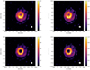 |
Fig. 3 Image reconstruction of HD 101584 without (left) and with (right) the significance contours at 5-σ
from bootstrapping. The top images are for |


5 Discussion
5.1 Rings are from thermal emission
First, we need to determine whether the origin of the rings’ emission is thermal or scattered light. Given the wavelength dependency of the visibilities in the H-band, we can estimate the black body temperature associated with each ring. We found low temperatures (1540 ± 10 K for the inner ring and 1014 ± 10 K for the outer one), making it unlikely that scattered light dominates the emission, as it would have a bluer spectrum similar to the stellar one. We note that 9.1 ± 0.1% of the flux is coming from an over-resolved component. However, its spectral index indicates a low temperature (T ~ 1290 K), which is also not compatible with scattered stellar light.
The orientation (inclination and PA) of the rings fits the results from the large-scale ALMA dataset well (HVO; 5° < i < 20°; PA ~ 90°; Olofsson et al. 2019). The PA, 9°, is essentially orthogonal to that of the HVO, suggesting an orientation of the rings in the equatorial plane of the outflow. We are, therefore, likely tracing the inner parts of the equatorial plane as seen with ALMA.
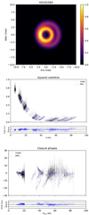 |
Fig. 4 Best-fit model of HD 101584. Top panel: image of the best-fit geometrical model. A comparison between the best-fit model and V2 and CP data are shown in the central and bottom panels, respectively. |
5.2 Rings in the same plane?
The structures of the circumstellar environment, as resolved in this object, are complex. Here, we review the underlying midplane structures that could give such an image in the near-infrared.
Both rings could be made by different mass loss episodes. Such a scenario was proposed to explain the double ring morphology in the equatorial plane of the Butterfly Nebula that was was detected in 12CO J = 2–1 and 12CO with the Institut de Radioastronomie Millimétrique (IRAM) Plateau de Bure interferometer, and in 13CO J = 3–2 with ALMA(Castro-Carrizo et al. 2012, 2017). Its large-scale hourglass-shaped outflow is similar to that of HD 101584 but is seen edge-on. However, the scale of the rings of HD 101584 (diameters of ~7 and ~13 au for a distance of 1.8 kpc) are very different from those of the Butterfly Nebula, whose rings have diameters of ~2600 and ~5200 au (for the adopted distance of 650 pc). It is interesting to note that the Butterfly Nebula rings are offset by ~130 au; these rings are possibly related to the hourglass-shaped structures seen in the scattered light images from the HST (Clyne et al. 2015). The Butterfly Nebula has a lower estimated mass (nebular mass of ~ 10−4 M⊙) than the environment of HD 101584 by at least an order of magnitude (the mass of the CCS alone is estimated to be about 10−3 M⊙). The different scales and the absence of dust thermal emission in the Butterfly Nebula make the link with the structure we observe weak. Furthermore, we lack kinematical information and cannot therefore conclude on a similar origin for the rings in the case of HD 101584. It is possible that at least one of the rings around HD 101584 is due to a mass loss event. This can be probed by re-imaging the target at an additional epoch in a search for dynamical changes.
Icke (2003) argued that multi-polar circumstellar nebulae, which seem to be seen around HD 101584 (Olofsson et al. 2019), can arise from the interaction of the wind with a warped circumstellar or circumbinary disk structure. Our data do not show strong evidence for such a warp as both rings are compatible with having the same orientation.
A binary system would likely induce a spiral wave in the circumbinary disk. From the images in Fig. 3, one could argue that the outer ring could in fact be a spiral originating from the eastern side that develops through the south to the west. This may, in principle, be possible if the disk is optically thin. Detailed radiative transfer modeling of this dataset is beyond of the scope of this paper. However, the radiative transfer model that was set to reproduce the SED, the ALMA continuum observations, and the rough size from near-infrared interferometry (the inner rim has a diameter of 4.3 mas in this model; Olofsson et al. 2019) show that the inner disk region is dense enough to be radially optically thick, meaning that the rest of the disk is shadowed from the star by the inner disk. It results in a sharp temperature drop behind the rim. Such a result is also recovered when modeling circumbinary disks around post-AGB objects from near-infrared interferometric data (Hillen et al. 2015; Kluska et al. 2018). Any structure behind the rim would not be detected in the H-band. A more refined model taking into account the more complex morphology revealed in this work would need to be constructed to further investigate this hypothesis.
5.3 A disk inner rim and an out-of-plane ring?
An alternative interpretation is that one of the rings is not in the midplane. Such a geometry may explain the shift between the two rings as observed in the image. The ring in the midplane would then trace the disk’s inner rim that is likely ruled by dust sublimation (Kluska et al. 2019). As we do not have unambiguous information on which of the rings is above the midplane, we will considertwo interpretations. Interpretation A treats the case where the inner disk is in the midplane; interpretation B treats the case of the outer ring being in the midplane (see Fig. 5). For each of the interpretations, we work out the three-dimensional configuration and the temperature of the dust located at different distances from the stars.
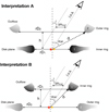 |
Fig. 5 Sketch of the two proposed interpretations. The evolved star is indicated by the red star and the unseen companion by the yellow disk. |
5.3.1 Interpretation A: inner ring in the midplane
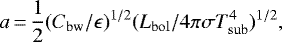
In this interpretation, we assume that the inner ring is the disk’s inner rim that would be at the dust sublimation radius, as in most of the similar post-AGB binary targets (Kluska et al. 2019). Knowing the stellar luminosity, one can use the following equation to determine the dust sublimation radius (Monnier & Millan-Gabet 2002; Lazareff et al. 2017):
 (1)
(1)
where Tsub is the sublimation temperature, Cbw is the back-warming coefficient (Kama et al. 2009), ɛ = Qabs(Tsub)∕Qabs(T*) is the dust grain cooling efficiency (which is the ratio of Planck-averaged absorption cross-sections at the dust sublimation and stellar temperatures), and σ is the Stefan-Boltzmann constant. The luminosity of the central star was determined to be 1600 L⊙ (assuming a distance of D = 1 kpc; Olofsson et al. 2019). Assuming Qabs(Tsub)∕Qabs(T*) = 1 and the back-warming coefficient being Cbw = 1, the theoretical dust sublimation radius would be 2.5 or 1.4 [D/1kpc] au for a dust sublimation temperature of 1000 and 1500 K, respectively; these are roughly the near-infrared emission temperatures found in post-AGB binaries (Kluska et al. 2019) and around young stars (Lazareff et al. 2017), respectively. The measured inner rim radius, 2.0 [D/1kpc] au, falls between the above estimates. While this is a standard size for inner rims of protoplanetary disks, the size is usually slightly larger for most post-AGB circumbinary disks (similar to the object of this study; see Fig. 6). Nevertheless, HD 101584 does not stand out, and we can assume that the inner disk rim is ruled by dust sublimation physics.
The outer ring has a temperature that is lower than that of the inner ring. We interpret the shift of the outer ring with respect to the inner ring as a geometrical effect due to the system inclination (see Fig. 5). One can therefore compute the height of the outer ring above the midplane (h) as being h = ΔRring2∕tani. This results in a height of 1.6 [D/1kpc] au. We can then verify the thermal emission origin of the outer ring by computing its distance to the central star, assuming it is located at the center of the inner ring. This distance is 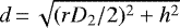 , which gives 4.1 [D/1kpc] au. If we assume that the emission of both rings comes from thermal emission of dust with similar characteristics (opacity, density), we can predict the distance to the outer ring knowing its temperature as
 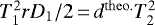 . In that case, dtheo. = 4.5 [D/1kpc] au, which is reasonably close to the estimated geometrical distance, albeit slightly larger. The slight difference (~10%) between d and dtheo. could be explained by a higher density at the location of the second ring, different dust properties, or uncertainties regarding the inclination and size estimations. In this case, we suggest that the outer ring is part of the outflow (see below).
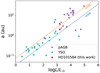 |
Fig. 6 Locating HD 101584 on the size-luminosity diagram from Kluska et al. (2019) for the two interpretations discussed in Sect. 5.3. |
5.3.2 Interpretation B: outer ring in the midplane
In this interpretation, we assume that the outer ring lies in the midplane. This would put the size of the disk’s inner rim at higher values, with a radius of 3.7 [D/1kpc] au, more compatible with most of the post-AGB circumbinary disks’ inner rims (Fig. 5). The height of the inner ring above the midplane is in this case 1.6 [D/1kpc] au. We then performed the same computations as for interpretation A but reversing the positions of the rings. Therefore, the distance of the inner rim to the central star would be  , which gives 2.5 [D/1kpc] au. As we did for interpretation A, we can estimate the distance of the second ring to the central star assuming similar dust characteristics for both rings as
  . For interpretation B,
  [D/1kpc] au; that is to say, we find a larger difference (~56%) compared to the geometrical distance (d = 2.5 [D/1kpc] au) than for interpretation A (see Table 2).
5.3.3 Interpretation A is more likely
From our dataset, we deduce that the inner ring represents 42% of the total H-band flux and ~58% of the circumstellar flux. Therefore, it dominates the H-band emission. Moreover, a model of a disk with an inner radius at 2.15 au successfully reproduces the SED at near-infrared wavelengths (Olofsson et al. 2019), which is very close to the inner ring radius we observe. Furthermore, the inner ring is more centered on the point source than the outer ring. These arguments strongly support interpretation A.
In both interpretations we can estimate the geometrical distance from the star to the ring that is out of the midplane. We also measure the temperatures of these rings. Assuming an optically thin inner cavity and thermal equilibrium, the energy received by a ring at a certain distance of the star can be translated to a ring temperature using Eq. (1). For interpretation A, the theoretical temperature is estimated to be 1068 K, which is remarkably close to the measured temperature (T2 = 1014 K). For interpretation B, the difference is larger since the theoretical temperature is 1743 K, which is 200 K above the measured one. This result also makes interpretation A more likely.
Finally, the blue-shifted part of the large-scale structure seen with ALMA is pointing in the western direction. If the large- and small-scale structures are linked, such an orientation agrees with interpretation A, where the out-of-plane structure is shifted in the western direction, and we do not detect its counterpart (in the red-shifted part), possibly because of the extinction caused by the disk.
5.4 Why do we not detect the companion?
Binarity is suggested by the periodicity seen in photometric and spectroscopic times series. Bakker et al. (1996) found a significant photometric period of 218d that is also tentatively found in radial velocities, but the low number of epochs and the line asymmetries could cause a bias in the obtained velocities. The fit was done for a circular orbit, but an eccentric one could have given better results. Pulsation and stellar rotation were ruled out by Bakker et al. (1996) because of the period and amplitude of the radial velocity variations. Bakker et al. (1996) argued that the photometric variability could be due to the periodic obscuration of the secondary continuum source (e.g., by a circumsecondary accretion disk). Given the orientation of the disk, it would imply that the binary is strongly misaligned with the disk. Another periodicity (144d) was estimated by Díaz et al. (2007) from spectroscopic data, but the data were never shown. This period is not compatible with the one from Bakker et al. (1996). It therefore remains possible that there is no secondary component in the system. In the following, we estimate the constrains we can bring from the non-detection of the companion assuming it is a binary system. A low-mass stellar companion would not be detected due to the high contrast with the evolved star. However, the near-infrared continuum emission at the position was detected in the case of the post-AGB binary system IRAS 08544-4431 (Hillen et al. 2016) and was interpreted as coming from a circumsecondary accretion disk. We therefore could also expect such a detection in HD 101584.
The evolutionary status of this object is unclear. Olofsson et al. (2019) claim that the object is most likely a post-RGB binary rather than a post-AGB binary. The different evolutionary scenarios lead to different distance and mass estimations, and the following two scenarios were considered. In the post-RGB case, the system would be 0.56 kpc away with a present day primary mass (M1) of 0.36 M⊙, whereas a post-AGB binary would be located at 1.8 kpc and the primary would have a present day mass of 0.55 M⊙.
The binary angular separation would be different in the two scenarios, and we want to investigate whether the non-detection of the secondary can place a constraint on its evolutionary status. From our observations, we find that the inclination of the disk is 20°, whereas the analysis of the HGS seen in the ALMA data points toward an inclination of 10°. Hereafter, we assume that the orbital plane of the putative companion is in the disk plane and that the orbit is circular. All these parameters influence the angular binary separation. We therefore computed the angular separations for each case.
We first estimated the mass function (f(M)) for each reported period using:
 (2)
(2)
where K1 = 3 km s−1 is the velocity semi-amplitude, P the orbital period, and G the gravitational constant. We then found the mass of the companion (M2) by solving:
 (3)
(3)
Then, we got the semimajor axis of the primary (a1) via:
![Mathematical equation: \begin{equation*} a_1\,{=}\,\sqrt[\leftroot{-1}\uproot{2}\scriptstyle 3]{\frac{f(M) G P^2}{4 \pi^2}} \frac{1}{\sin i} .\end{equation*}](/articles/aa/full_html/2020/10/aa37946-20/aa37946-20-eq35.png) (4)
(4)
We computed the semimajor axis of the secondary (a2) with:
 (5)
(5)
We obtained the physical separation by adding the two semimajor axes. Finally, we used the distance (D) to get the angular separation (ρ):
 (6)
(6)
The results for each case and each computation step are presented Table 3.
The maximum angular distance is given by the post-RGB scenario with a period of 218d and an inclination of 10°. This separation of 1.2 mas is of the same order as our maximum resolution power: λ∕2Bmax ~ 1.3 mas. Our observations therefore do not constrain the binary separation and cannot exclude either of the two evolutionary scenarios proposed in Olofsson et al. (2019), irrespective of its contribution to the H-band flux.
Parameters of the orbital separation taking into account the different scenarios.
6 Conclusions
The conclusions we have obtained from the HD 101584 VLTI/PIONIER data analysis are:
- 1.
The reconstructed image from VLTI/PIONIER observations of the environment of HD 101584 reveals an unexpected double ring morphology.
- 2.
Both rings are compatible with a dust sublimation rim but at different temperatures.
- 3.
The two rings are not concentric. We postulate that the shift between the two rings is compatible with a projection effect where one of the two rings is not in the midplane. The height (h) of the ring that is out of the midplane is 1.6[D/1kpc] au. The ring that is out of the plane may be linked with the hourglass-shaped outflow seen on a large scale with ALMA.
- 4.
The origin of the out-of-plane ring is unclear. It is shifted in the direction of the blue-shifted part of the outflow seen by ALMA (i.e., the part of the outflow moving toward us). We speculate that it is tracing either a density enhancement or the dust condensation front in the outflow. We propose additional infrared interferometric observations of this target to discriminate between these two hypotheses.
- 5.
The non-detection of the secondary is compatible with the post-RGB, post-AGB, and merger evolutionary scenarios of this object.
High-angular observations in the infrared are able to image the stellar environments at an astronomical-unit scale, allowing us to probe important processes in the evolution of binary stars or mergers. The imaging approach is crucial for revealing unexpected features andguiding the interpretation and modeling of a complex circumstellar and circumbinary environment. The secondary ring detected in HD 101584 is certainly unexpected. Thanks to observations at larger scales, one can now study these objects thoroughly and link morphological features observed at different scales (HST, ALMA) to constrain the complex physical processes at play in circumstellar environments. To confirm our out-of-plane scenario, we propose to re-observe this target at the same wavelengths as well as at longer infrared wavelengths (with GRAVITY or MATISSE at the VLTI) to probe its density structure and understand its launching mechanism and impact on the fate of the system.
Acknowledgements
We want to thank the referee for comments that improved the manuscript. J.K. and H.V.W. acknowledge support from the research council of the KU Leuven under grant number C14/17/082. H.O. and W.V. acknowledge financial support from the Swedish Research Council.
Appendix A Log of the observations
The log of the observations is indicated in Table A.1.
Log of observations.
Appendix B Chromatic parameters determination
To determine the optimal chromatic parameters, we made a grid of 50 × 50 pairs of  and denv. We reconstructed an image for each pair of parameters, and we selected the pair for which the cost f is the lowest. We varied
  between 0.15 and 0.35 and denv between −1 and 5.
The second image reconstruction presented in Sect. 4 was done by setting the stellar-to-total flux ratio ( ) to 0.28 andmaking a grid on the spectral index of the environment (denv). This linear grid was made of 200 values between −3.1 and 4.9 (corresponding to black body temperatures between the one of the star and 880 K). We find denv = 1.75 as the most likely value, which is compatible with the grid on both chromatic parameters made in the first step (Fig. 2).
Appendix C Effect of the regularization weight
The L-curve used in the image reconstruction of Sect. 3 is shown in Fig. C.1. We distinguish the two regimes of the L curve. In the low μ case, the L curve is not smooth, probably because of local minima due to the interferometric data (e.g., not convexity due to phases).
To illustrate our exploration of the regularization weight parameter, we show in Fig. C.2 how the image changes with the regularization weight for a constant  (
( = 0.28). As an illustration, we also indicated the reduced χ2 (even though it is not the value that is reduced when optimizing the image) that increases for higher regularization weights (μ > 109) as expected when switching from a regime that minimizes the likelihood to a regime dominated by the regularization cost.
We can see that the global characteristics of the image are retrieved, namely a bright inner ring and an extendedstructure that looks like an outer ring slightly shifted toward the west. For higher regularization weights, the outer ring becomes an arc in the western direction. Because of the smoothness regularization used, the emission from the eastern side of the ring became super-imposed with the inner rim. Images with higher μ do not change our interpretation, as we can still model the data with the double ring morphology.
We also tested the effect of a different regularization. We used the total variation regularization (Renard et al. 2010). This regularization reduces the number of gradients in the image. By doing this it will create plateaus in the image. This regularization is not quadratic and is more likely to fall in a local minimum than the quadratic smoothness regularization. The images obtained with this regularization show similar features (see Fig. C.3), namely the inner ring and the secondary ring that is closer to theinner ring on the eastern side.
 |
Fig. C.2 Image reconstructions using different regularization weights. The images are made using
|

 |
Fig. C.3 Image reconstructions using the total variation regularization with different regularization weights. The images are made using |

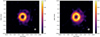 |
Fig. C.4 Image reconstructions using the quadratic smoothness regularization with the three shortest-wavelength channels (left) and the three longest-wavelength ones (right). The images are made using
|

Finally, Fig. C.4 shows image reconstructions when the dataset is split between the channels with shorter wavelengths (λ < 1.65 μm) and those with longer ones (λ >1.65 μm). More artifacts are expected because we divide the number of data points by a factor of two and the beam size is different in the two images (the image with shorter wavelengths will have a better angular resolution). We recover the ring in both images together with the west-side arc, although beam size effects are visible. The east-side part of the outer ring is seen for the shortest wavelengths only, where higher angular resolution is needed, although its structure is distorted.
Appendix D Fit of the images to the dataset
The comparison of the interferometric observables from the images to the dataset are shown in Figs. D.1 and D.2 for the image reconstruction. In Fig. D.1,  = 0.244 and denv = 2.45, and in Fig. D.2,
  = 0.28 and denv = 1.75.
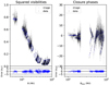 |
Fig. D.1 Comparison of the observables from the image reconstruction of HD 101584 done in Sect. 3 with chromatic parameters being |

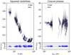 |
Fig. D.2 Comparison of the observables from the image reconstruction of HD 101584 done in Sect. 4 with chromatic parameters being |

Appendix E Geometrical model
The geometrical model is inspired by the reconstructed image. Because of the linearity of the Fourier transform, the model can be defined as the flux weighted sum of individual components. It is made of a point source to reproduce the star, two rings, and a background to take into account the over-resolved flux. The two rings’ orientation is defined with the same inclination and PA. Moreover, both the point source and the outer ring can be shifted with respect to the inner ring. Hereafter, we mathematically describe the geometrical model we used to reproduce the interferometric data.
To combine the different components of the model, one needs to define the fluxes of each component. Those fluxes are normalized and positive. They have to respect the following constraints:

where  is the flux ratio of the ith component (here it can be the star, one of the rings, or the background flux) at 1.65 μm. To extrapolate the flux ratios to other wavelengths (fi) probed by the data, spectral laws are assigned to each component.
For both rings, a black body at temperature (Ti) is assigned, as follows:
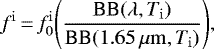 (E.4)
(E.4)
where BB is the Planck black body function and λ is the wavelength of an observation.
For the point source and the background, the spectrum is a power-law with a spectral index ( ) as follows:
 (E.5)
(E.5)
In the following, we describe the analytical Fourier transforms we used in the model. We describe each component separately.
-
The star:the visibility of a point source equals unity for every spatial frequency (V * = 1). The star can be shifted with respect to the inner ring center by Δx and Δy for right ascension and declination shift, respectively. Therefore, the complex visibility of the star is:
 (E.6)
(E.6)where u and v are the spatial frequencies in the west-east and south-north directions.
-
The ring: the ring is first defined as an infinitesimal ring distribution. Its visibility (V ring0(u, v)) equals:
 (E.7)
(E.7)where J0 is the Bessel function of the 0th order, rDi is the diameter of the ith ring, and ρ′ is the spatial frequency of a data point corrected for inclination (i) and PA of the ring as follows:

The ring is then convolved by a Gaussian such as:
 (E.11)
where rWi is the ratio of the ith ring full width at half maximum to its radius.
Additionally, for the second ring a phasor is added for its shift:
 (E.12)
with the ring shifts Δxring2 and Δyring2 defined as:

with ΔRring2 being the ring2 shift. Ring2 can therefore only be shifted in the direction of the minor axis.
-
The background: the extended flux is modeled by an over-resolved emission that has a null visibility.
-
The finalmodel: as the flux ratios of the three components are normalized to 1 at 1.65 μm (Eq. (E.1)),
 is defined as:
 (E.15)
The final visibility can therefore be written as a linear combination of the four components of the model as:
 (E.16)
 |
Fig. E.1 Corner plot from the MCMC fit. |
 |
Fig. E.2 Bessel functions of the rings and the star from the best-fit geometric model over data at 1.65 μm. Second-order variations due to the shift of the ring are not taken into account. The outer ring is plotted with a shift corresponding to the fluxes of the inner ring and the star flux ratios. The inner ring is plotted with a shift corresponding to the stellar flux ratio. There are no strong features in the visibilities at the location of the gaps in spatial frequencies. The spatial frequencies are in log scale. |
References
- Abate, C., Pols, O. R., Izzard, R. G., Mohamed, S. S., & de Mink, S. E. 2013, A&A, 552, A26 [NASA ADS] [CrossRef] [EDP Sciences] [Google Scholar]
- Bakker, E. J., Lamers, H. J. G. L. M., Waters, L. B. F. M., & Waelkens, C. 1996, A&A, 310, 861 [Google Scholar]
- Castro-Carrizo, A., Neri, R., Bujarrabal, V., et al. 2012, A&A, 545, A1 [NASA ADS] [CrossRef] [EDP Sciences] [Google Scholar]
- Castro-Carrizo, A., Bujarrabal, V., Neri, R., et al. 2017, A&A, 600, A4 [NASA ADS] [CrossRef] [EDP Sciences] [Google Scholar]
- Clyne, N., Akras, S., Steffen, W., et al. 2015, A&A, 582, A60 [NASA ADS] [CrossRef] [EDP Sciences] [Google Scholar]
- De Nutte, R., Decin, L., Olofsson, H., et al. 2017, A&A, 600, A71 [NASA ADS] [CrossRef] [EDP Sciences] [Google Scholar]
- Díaz, F., Hearnshaw, J., Rosenzweig, P., et al. 2007, IAU Symp., 240, 127 [NASA ADS] [Google Scholar]
- Duchêne, G., & Kraus, A. 2013, ARA&A, 51, 269 [Google Scholar]
- Eyres, S. P. S., Evans, A., Zijlstra, A., et al. 2018, MNRAS, 481, 4931 [NASA ADS] [Google Scholar]
- Foreman-Mackey, D., Hogg, D. W., Lang, D., & Goodman, J. 2013, PASP, 125, 306 [CrossRef] [Google Scholar]
- Fortin, F.-A., De Rainville, F.-M., Gardner, M.-A., Parizeau, M., & Gagné, C. 2012, J. Mach. Learn. Res., 13, 2171 [Google Scholar]
- Hillen, M., Menu, J., Van Winckel, H., et al. 2014, A&A, 568, A12 [NASA ADS] [CrossRef] [EDP Sciences] [Google Scholar]
- Hillen, M., de Vries, B. L., Menu, J., et al. 2015, A&A, 578, A40 [NASA ADS] [CrossRef] [EDP Sciences] [Google Scholar]
- Hillen, M., Kluska, J., Le Bouquin, J.-B., et al. 2016, A&A, 588, L1 [NASA ADS] [CrossRef] [EDP Sciences] [Google Scholar]
- Hillen, M., Van Winckel, H., Menu, J., et al. 2017, A&A, 599, A41 [NASA ADS] [CrossRef] [EDP Sciences] [Google Scholar]
- Icke, V. 2003, A&A, 405, L11 [NASA ADS] [CrossRef] [EDP Sciences] [Google Scholar]
- Ivanova, N., Justham, S., Chen, X., et al. 2013, A&ARv, 21, 59 [Google Scholar]
- Kama, M., Min, M., & Dominik, C. 2009, A&A, 506, 1199 [NASA ADS] [CrossRef] [EDP Sciences] [Google Scholar]
- Kamath, D., & Van Winckel, H. 2019, MNRAS, 486, 3524 [NASA ADS] [CrossRef] [Google Scholar]
- Kamath, D., Wood, P. R., & Van Winckel, H. 2015, MNRAS, 454, 1468 [NASA ADS] [CrossRef] [Google Scholar]
- Kamath, D., Wood, P. R., Van Winckel, H., & Nie, J. D. 2016, A&A, 586, L5 [NASA ADS] [CrossRef] [EDP Sciences] [Google Scholar]
- Karakas, A. I., & Lattanzio, J. C. 2014, PASA, 31, e030 [NASA ADS] [CrossRef] [Google Scholar]
- Kato, T. 2003, A&A, 399, 695 [NASA ADS] [CrossRef] [EDP Sciences] [Google Scholar]
- Kipper, T. 2005, Balt. Astron., 14, 223 [NASA ADS] [Google Scholar]
- Kluska, J., Malbet, F., Berger, J.-P., et al. 2014, A&A, 564, A80 [NASA ADS] [CrossRef] [EDP Sciences] [Google Scholar]
- Kluska, J., Benisty, M., Soulez, F., et al. 2016, A&A, 591, A82 [NASA ADS] [CrossRef] [EDP Sciences] [Google Scholar]
- Kluska, J., Hillen, M., Van Winckel, H., et al. 2018, A&A, 616, A153 [NASA ADS] [CrossRef] [EDP Sciences] [Google Scholar]
- Kluska, J., Van Winckel, H., Hillen, M., et al. 2019, A&A, 631, A108 [NASA ADS] [CrossRef] [EDP Sciences] [Google Scholar]
- Lazareff, B., Berger, J.-P., Kluska, J., et al. 2017, A&A, 599, A85 [NASA ADS] [CrossRef] [EDP Sciences] [Google Scholar]
- Le Bouquin, J.-B., Berger, J.-P., Lazareff, B., et al. 2011, A&A, 535, A67 [NASA ADS] [CrossRef] [EDP Sciences] [Google Scholar]
- Monnier, J. D., & Millan-Gabet, R. 2002, ApJ, 579, 694 [NASA ADS] [CrossRef] [Google Scholar]
- Olofsson, H., Vlemmings, W. H. T., Maercker, M., et al. 2015, A&A, 576, L15 [NASA ADS] [CrossRef] [EDP Sciences] [Google Scholar]
- Olofsson, H., Vlemmings, W. H. T., Bergman, P., et al. 2017, A&A, 603, L2 [NASA ADS] [CrossRef] [EDP Sciences] [Google Scholar]
- Olofsson, H., Khouri, T., Maercker, M., et al. 2019, A&A, 623, A153 [CrossRef] [EDP Sciences] [Google Scholar]
- Pastorello, A., Mason, E., Taubenberger, S., et al. 2019, A&A, 630, A75 [NASA ADS] [CrossRef] [EDP Sciences] [Google Scholar]
- Renard, S., Malbet, F., Benisty, M., Thiébaut, E., & Berger, J.-P. 2010, A&A, 519, A26 [NASA ADS] [CrossRef] [EDP Sciences] [Google Scholar]
- Renard, S., Thiébaut, E., & Malbet, F. 2011, A&A, 533, A64 [NASA ADS] [CrossRef] [EDP Sciences] [Google Scholar]
- Sahai, R., Vlemmings, W. H. T., & Nyman, L. Å. 2017, ApJ, 841, 110 [NASA ADS] [CrossRef] [Google Scholar]
- Sana, H., Le Bouquin, J. B., Lacour, S., et al. 2014, ApJS, 215, 15 [Google Scholar]
- Shara, M. M., Moffat, A. F. J., & Webbink, R. F. 1985, ApJ, 294, 271 [NASA ADS] [CrossRef] [Google Scholar]
- Sivarani, T., Parthasarathy, M., García-Lario, P., Manchado, A., & Pottasch, S. R. 1999, A&AS, 137, 505 [NASA ADS] [CrossRef] [EDP Sciences] [Google Scholar]
- Thiébaut, E. 2008, SPIE Conf. Ser., 7013, 1 [Google Scholar]
- Van Winckel, H. 2003, ARA&A, 41, 391 [NASA ADS] [CrossRef] [Google Scholar]
- Van Winckel, H. 2018, ArXiv e-prints, [arXiv:1809.00871] [Google Scholar]
As mentioned, throughout the paper we give quantities for a reference distance of 1 kpc followed by the scaling of these quantities with distance given in squared brackets.
All Tables
Parameters of the orbital separation taking into account the different scenarios.
All Figures
|
Fig. 1 VLTI/PIONIER dataset on HD 101584. Top: obtained (u, v)-coverage. Center: V2 against spatial frequency. Bottom: CP against the highest spatial frequency of a closure triangle. Spatial frequency is in log-scale. The color indicates the wavelength. |
| In the text | |
|
Fig. 2 Logarithm of the cost function f as a function of the chromatic parameters |
| In the text | |
|
Fig. 3 Image reconstruction of HD 101584 without (left) and with (right) the significance contours at 5-σ
from bootstrapping. The top images are for |
| In the text | |
|
Fig. 4 Best-fit model of HD 101584. Top panel: image of the best-fit geometrical model. A comparison between the best-fit model and V2 and CP data are shown in the central and bottom panels, respectively. |
| In the text | |
|
Fig. 5 Sketch of the two proposed interpretations. The evolved star is indicated by the red star and the unseen companion by the yellow disk. |
| In the text | |
|
Fig. 6 Locating HD 101584 on the size-luminosity diagram from Kluska et al. (2019) for the two interpretations discussed in Sect. 5.3. |
| In the text | |
 |
Fig. C.1 L-curve for the image reconstruction displayed in Fig. 3. |
| In the text | |
|
Fig. C.2 Image reconstructions using different regularization weights. The images are made using
|
| In the text | |
|
Fig. C.3 Image reconstructions using the total variation regularization with different regularization weights. The images are made using |
| In the text | |
|
Fig. C.4 Image reconstructions using the quadratic smoothness regularization with the three shortest-wavelength channels (left) and the three longest-wavelength ones (right). The images are made using
|
| In the text | |
|
Fig. D.1 Comparison of the observables from the image reconstruction of HD 101584 done in Sect. 3 with chromatic parameters being |
| In the text | |
|
Fig. D.2 Comparison of the observables from the image reconstruction of HD 101584 done in Sect. 4 with chromatic parameters being |
| In the text | |
|
Fig. E.1 Corner plot from the MCMC fit. |
| In the text | |
|
Fig. E.2 Bessel functions of the rings and the star from the best-fit geometric model over data at 1.65 μm. Second-order variations due to the shift of the ring are not taken into account. The outer ring is plotted with a shift corresponding to the fluxes of the inner ring and the star flux ratios. The inner ring is plotted with a shift corresponding to the stellar flux ratio. There are no strong features in the visibilities at the location of the gaps in spatial frequencies. The spatial frequencies are in log scale. |
| In the text | |
Current usage metrics show cumulative count of Article Views (full-text article views including HTML views, PDF and ePub downloads, according to the available data) and Abstracts Views on Vision4Press platform.
Data correspond to usage on the plateform after 2015. The current usage metrics is available 48-96 hours after online publication and is updated daily on week days.
Initial download of the metrics may take a while.