| Issue |
A&A
Volume 642, October 2020
|
|
|---|---|---|
| Article Number | A117 | |
| Number of page(s) | 6 | |
| Section | Stellar structure and evolution | |
| DOI | https://doi.org/10.1051/0004-6361/202037435 | |
| Published online | 12 October 2020 | |
Kilohertz quasi-periodic oscillations as probes of the X-ray color-color diagram and neutron star accretion-disk structure for Z sources
1
School of Physics and Electronic Science, Guizhou Normal University, Guiyang 550001, PR China
e-mail: This email address is being protected from spambots. You need JavaScript enabled to view it.
2
CAS key Laboratory of FAST, National Astronomical Observatories, Beijing 100101, PR China
e-mail: This email address is being protected from spambots. You need JavaScript enabled to view it.
3
School of Physical Sciences, University of Chinese Academy of Sciences, Beijing 100049, PR China
4
Key Laboratory of Radio Astronomy, Chinese Academy of Sciences, Beijing 100101, PR China
5
Institute of High Energy Physics, Chinese Academy of Sciences, Beijing 100049, PR China
Received:
1
January
2020
Accepted:
29
July
2020
Abstract
Based on the detected kilohertz quasi-periodic oscillations (kHz QPOs) in neutron star low-mass X-ray binaries (NS-LMXBs), we investigate the evolution of the NS magnetosphere-disk structure along the Z track in the X-ray color-color diagram (CCD) for luminous Z sources, such as Cyg X-2, GX 5-1, GX 17+2, and Sco X-1. We find that the magnetosphere-disk radius r inferred by kHz QPOs for all the sources shows a monotonically decreasing trend along the Z track from the horizontal branch (HB) to the normal branch (NB), implying that the dominated radiation components may dramatically change as the accretion disk moves toward the NS surface. In addition, the specific radius that corresponds to the HB/NB vertex is found to be around r ∼ 20 km, implying a potential characteristic position of transiting for the X-ray radiation mode. Furthermore, we find that the NBs that occur near the NS surface have a radius of r ∼ 16−20 km, which is systematically smaller than those of HBs that have radii of r ∼ 20−29 km. To interpret the relation between the CCD properties and the special magnetosphere-disk radii of Z sources, we suggest that the magnetic field lines corresponding to NB are “frozen-in” to the plasma, and move further inward with the shrinking of the NS magnetosphere-disk radius and pile up near the NS surface. They then form a strong magnetic field region around r ∼ 16−20 km, where the high magnetic energy density and high plasma mass density may dominate the radiation process in NB.
Key words: X-rays: binaries / stars: neutron / binaries: close / accretion, accretion disks
© ESO 2020
1. Introduction
Neutron star low-mass X-ray binaries (NS-LMXBs) can be classified into low luminosity atoll sources (LX ∼ 0.01−0.5 LEdd) and high luminosity Z sources (LX ∼ 0.5−1 LEdd) based on their patterns in the X-ray color-color diagrams (CCDs) or the hardness-intensity diagrams (HIDs; Hasinger & van der Klis 1989; van der Klis et al. 2006). The tracks of Z sources typically exhibit three branches called the horizontal branch (HB), normal branch (NB), and flaring branch (FB), while the tracks of atoll sources are called the extreme island, island, lower banana, and upper banana state. Unlike the above typical behaviors of atoll and Z sources, the transition between the atoll and Z tracks has been observed in XTE J1701-462 (Homan et al. 2007, 2010; Lin et al. 2009; Fridriksson et al. 2015). In both atoll and Z sources the evolution of temporal and spectral features along the tracks in the CCD have been observed, and the typical frequencies of most timing variability components of Z sources increase from the HB to NB (Homan et al. 2007). The NS millisecond spin signals have been detected in several atoll sources, however, no NS spin frequency has been detected in Z sources (van der Klis 2016; Wang et al. 2018a). Several physical effects, such as the mass accretion rate (Hasinger 1990; Hasinger et al. 1990) and the NS magnetic field (Hasinger & van der Klis 1989), have been proposed to explain the differences between the two subclasses of sources, however, there is no consensus as to their origins.
Twin kilohertz quasi-periodic oscillations (kHz QPOs) have been detected both in atoll and Z sources by the Rossi X-ray Timing Explorer (RXTE; van der Klis et al. 2006). These high frequency QPOs usually appear in pairs (lower ν1 and upper ν2) in the frequency range of ≃100−1300 Hz (Wang et al. 2014), and show a nonlinear relation between ν1 and ν2 (Belloni et al. 2005, 2007; Zhang et al. 2006). The frequencies of kHz QPOs often increase monotonically along both the atoll tracks (e.g., Méndez et al. 1999; Di Salvo et al. 2001; van Straaten et al. 2000, 2003; Altamirano et al. 2008) and Z tracks (e.g., van der Klis et al. 1996; Wijnands et al. 1997a, 1998a,b; Homan et al. 2002; Jonker et al. 2002; Lin et al. 2012), which also show an indirect correlation with the NS spin frequency, and with other temporal and spectral features (e.g., Ford & van der Klis 1998; Jonker et al. 1998; Kaaret et al. 1998; Psaltis et al. 1999; Belloni et al. 2002; Di Salvo et al. 2003; Méndez 2006; Ribeiro et al. 2017; Zhang et al. 2017; Troyer et al. 2018; van Doesburgh & van der Klis 2019). In particular, the same kHz QPO frequency could correspond to at least two different luminosities and colors, known as the phenomenon of “parallel tracks” (Méndez & van der Klis 1999; Ford et al. 2000; Méndez et al. 2001; van der Klis 2001). It is suggested that kHz QPOs may reflect the orbital motion of the accreting matter at the inner accretion disk (van der Klis 2000; Kluźniak et al. 2004; Kluźniak 2005; Zhang & Wang 2013), which can be exploited to explore the physical environments in the strong gravitational field and strong magnetic field regions (Miller et al. 1998; Stella & Vietri 1999; Stella et al. 1999; Lamb & Miller 2001; Abramowicz et al. 2003a,b; Zhang 2004), to probe the magnetosphere-disk structure of NS-LMXBs (Wang et al. 2018b), and to constrain the NS Mass − Radius relation (Miller & Miller 2015; Török et al. 2016, 2019; van Doesburgh et al. 2018).
Based on the kHz QPO data and NS spin frequencies of atoll sources, Wang et al. (2017) analyzed the relation between the kHz QPO emission radius and the co-rotation radius of NS-LMXBs, and found that the twin kHz QPOs may originate from the NS spin-up state, while the magnetosphere-disk is trapped within the NS co-rotation radius. Furthermore, Wang et al. (2018b) probed the magnetosphere-disk structure evolution of the atoll source 4U 1728-34 using kHz QPOs, and found that the accretion disk moves toward the NS surface as the atoll track evolves from the island state to the banana state, where the magnetic field strength at the inner accretion disk increases by one order of magnitude. The Z sources have also been detected by kHz QPOs in the different positions of the HB and NB based on a measurement of the position parameter. Motivated by the work of Wang et al. (2018b) on atoll sources, we try to analyze the evolution of the magnetosphere-disk structure of the Z sources along the X-ray CCD tracks using kHz QPOs, and further investigate the effects of the accretion and magnetic field environment on the formation of the Z track.
The paper is organized as follows. In Sect. 2, we introduce the samples of Z sources and their Z-track parameters with kHz QPOs for Cyg X-2, GX 5-1, GX 17+2, and Sco X-1. In Sect. 3, we infer the kHz QPO emission radii of these Z sources and probe their evolution paths along the Z tracks. In Sect. 4, we present the discussions and conclusions.
2. Samples of Z sources and their Z-track parameters with kHz QPOs
2.1. Description of Sz parameter
The Z source usually traces the “Z” track in the CCD or HID, and its position along the track can be parameterized by the Sz value (see, e.g., Hasinger et al. 1990; Wijnands et al. 1997b). In this method, all the points in the CCD are projected onto a bicubic spline, where the HB/NB and NB/FB vertices are given the value of Sz ∼ 1 and Sz ∼ 2, respectively. The remaining points of the Z track are scaled according to the length of the NB. This method defines the measure of the curve length, so Sz < 1 and Sz > 2 are not the special points or vertices.
2.2. Published samples of Sz and kHz QPOs
We searched the published literature for the Z sources that have detected kHz QPOs at the different positions of the Z track based on the Sz parameterization, and constrained the samples to those with detected kHz QPOs on the NB. There are four Z sources that satisfy the conditions: Cyg X-2, GX 5-1, GX 17+2, and Sco X-1. We collected the upper kHz QPO frequency ν2 and the corresponding Sz values of these sources from the literature (a total of 97 pairs of data, as shown in Table 1), and the details of the observations are as follows:
Frequencies and inferred emission radii of the kHz QPOs.
– Cyg X-2: Wijnands et al. (1998a) analyzed the RXTE data of Cyg X-2 from 1997 June 30 to July 3, with a total observation time of ∼108 ks. The authors detected kHz QPOs at the different positions of the HB and NB using the Sz parameterization. We obtained the Sz and ν2 values from Fig. 3 of Wijnands et al. (1998a) in the range of Sz ∼ −0.09−1.13 and ν2 ∼ 735−1015 Hz, respectively (see Table 1).
– GX 5-1: (I). Wijnands et al. (1998b) analyzed the RXTE data of GX 5-1 on 1996 November 2, 6, and 16, and on 1997 May 30, June 5, and July 25, with a total observation time of ∼102 ks. The authors detected kHz QPOs at the different positions of the HB and NB using the Sz parameterization. We obtained the Sz and ν2 values from Fig. 3 of Wijnands et al. (1998b) in the range of Sz ∼ 0.67−1.25 and ν2 ∼ 507−888 Hz, respectively (see Table 1). (II). Jonker et al. (2002) analyzed the 76 pieces of RXTE data relating to GX 5-1 that span 1996 July 27 to 2000 March 3, with a total observation time of ∼564 ks. The authors detected kHz QPOs at the different positions of the HB and NB using the Sz parameterization. We obtained the Sz and ν2 values from Table 4 of Jonker et al. (2002) in the range of Sz ∼ 0.12−1.10 and ν2 ∼ 478−866 Hz, respectively (see Table 1). Most of the RXTE data analyzed by Wijnands et al. (1998b) on GX 5-1 is included in Jonker et al. (2002).
– GX 17+2: (I). Wijnands et al. (1997a) analyzed the RXTE data of GX 17+2 on 1997 February 6–8, April 1–4, and July 26–27, with a total observation time of ∼120.5 ks. The authors detected kHz QPOs at the different positions of the HB and NB using the Sz parameterization. We obtained the Sz and ν2 values from Fig. 3 of Wijnands et al. (1997a) in the range of Sz ∼ 0.08−1.45 and ν2 ∼ 647−1087 Hz, respectively (see Table 1). (II). Homan et al. (2002) analyzed the RXTE data of GX 17+2 between 1997 February 2 and 2000 March 31, with a total observation time of ∼600 ks. The authors detected kHz QPOs at the different positions of the HB and NB using the Sz parameterization. We obtained the Sz and ν2 values from Table 8 of Homan et al. (2002) in the range of Sz ∼ −0.32−1.76 and ν2 ∼ 618−1087 Hz, respectively (see Table 1). (III). Lin et al. (2012) analyzed the 68 RXTE observations of GX 17+2 between 1999 October 3 and 12, with a total observation time of ∼270 ks. The authors detected kHz QPOs at the different positions of the HB and NB using the Sz parameterization. We obtained the Sz and ν2 values from Table 3 of Lin et al. (2012) in the range of Sz ∼ 0.16−1.16 and ν2 ∼ 623−963 Hz, respectively (see Table 1). Most of the RXTE data analyzed by Wijnands et al. (1997a) and Lin et al. (2012) on GX 17+2 is included in Homan et al. (2002).
– Sco X-1: van der Klis et al. (1996) analyzed the RXTE observations of Sco X-1 on 1996 February 14 from 0914 to 1325 UT, February 18 0446−0840 UT, and February 19 1009−1456 UT. The authors detected kHz QPOs at the different positions of the NB using the Sz parameterization. We obtained the Sz and ν2 values from Table 1 of van der Klis et al. (1996) in the range of Sz ∼ 1.25−2.09 and ν2 ∼ 1050−1135 Hz, respectively (see Table 1).
We tried to illustrate the Z tracks of the above sources in HIDs, and collected the same RXTE data as that in Wijnands et al. (1998a) for Cyg X-2 (in gain epoch 3), Jonker et al. (2002) for GX 5-1 (in gain epochs 3 and 4), Homan et al. (2002) for GX 17+2 (in gain epochs 3 and 4), and van der Klis et al. (1996) for Sco X-1 (in gain epoch 1). Then, we extracted the light curves of these data with Standard 2 mode from Proportional Counter Unit (PCU) 2, where the background is subtracted by the bright source model. We define the hard color as the ratio of the count rate in the bands 9.8−15.9 keV/6.5−9.8 keV for Cyg X-2, GX 5-1, and GX 17+2, and 9.8−15.9 keV/6.4−9.8 keV for Sco X-1, while the corresponding X-ray intensities are defined as the count rate in 1.9−15.9 keV for Cyg X-2, GX 5-1, and GX 17+2, and 2.0−15.9 keV for Sco X-1. The data of both GX 5-1 and GX 17+2 are in the two gain epochs of 3 and 4. Then, in order to correct the colors and intensities for the instrumental response changes in the different gain epochs, we calculated the colors and intensities of the Crab Nebula with PCU2 in the same energy bands of gain epochs 3 and 4, which can be supposed to be constant, and inferred the corresponding correction factors between epochs 3 and 4 (van Straaten et al. 2000). Finally, we applied these Crab correction factors to convert the hard colors and X-ray intensities of GX 5-1 and GX 17+2 in epoch 4 to match those in epoch 3. Furthermore, considering that dead-time has a significant effect on the count rate for Z sources (see, e.g., van der Klis et al. 1996; Wijnands et al. 1997a, 1998a; Jonker et al. 1998; Méndez & van der Klis 2000), we calculated the dead-time fractions (DTFs) of PCU2 for the observed data, which share the range of ∼2−4%, ∼3−6%, ∼3−6%, and ∼22−30% for Cyg X-2, GX 5-1, GX 17+2, and Sco X-1, respectively. Then, we corrected the dead-time for the count rates in light curves of each source with the corresponding averaged DTFs. The schematic diagrams of the Z tracks in the HIDs of these sources are shown in Fig. 1, where the approximate positions that correspond to the HB/NB vertex (Sz ∼ 1) and NB/FB vertex (Sz ∼ 2) are also indicated.
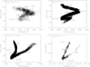 |
Fig. 1. Schematic diagrams of the Z tracks in the hardness-intensity diagrams, for (a) Cyg X-2, (b) GX 5-1, (c) GX 17+2, and (d) Sco X-1, where the approximate positions of the HB/NB vertex (Sz ∼ 1) and NB/FB vertex (Sz ∼ 2) are indicated by the parameter Sz as defined by Hasinger et al. (1990) and Wijnands et al. (1997b) (see the text). On the axis quantities of the diagrams, the hard colors are defined as the ratio of the count rate in the bands of 9.8−15.9 keV/6.5−9.8 keV for Cyg X-2, GX 5-1, and GX 17+2, and 9.8−15.9 keV/6.4−9.8 keV for Sco X-1, while the X-ray intensities are defined as the count rate in 1.9−15.9 keV for Cyg X-2, GX 5-1, GX 17, and 2.0−15.9 keV for Sco X-1. The diagrams are produced with the same RXTE data as that in Wijnands et al. (1998a) for Cyg X-2, Jonker et al. (2002) for GX 5-1, Homan et al. (2002) for GX 17+2, and van der Klis et al. (1996) for Sco X-1. The hard colors are not dead-time corrected because of the small correction factors (< 0.2%). |
3. Evolution of the magnetosphere-disk structure along the Z track
3.1. Emission radius of the kHz QPO
In this paper, the upper kHz QPO frequency ν2 is assumed as the Keplerian orbital frequency νK,
 (1)
(1)
where G is the gravitational constant, M is the NS mass, and r is the emission radius of the kHz QPO referring to the NS center, which is the magnetosphere-disk radius. By solving Eq. (1), r can be derived as
 (2)
(2)
We infer the emission radii of the kHz QPOs in Table 1 using Eq. (2) with the detected ν2 values and the assumed NS mass of M ∼ 1.6 M⊙ (i.e., the average mass of the millisecond pulsars, see Zhang et al. 2011 and Özel & Freire 2016). The results are shown in Table 1, where it can be seen that Cyg X-2, GX 5-1, GX 17+2, and Sco X-1 share the r range of ∼17.4−21.5 km, ∼19.0−28.7 km, ∼16.6−24.1 km, and ∼16.1−17.0 km, respectively.
3.2. Relation between the magnetosphere-disk radius and Z track parameter
The cumulative distribution function (CDF) curves of the kHz QPO emission radius r of the Z sources in Table 1 are shown in Figs. 2a–g respectively, where the corresponding Z track parameter Sz values are also indicated. All the sources show a monotonically decreasing trend of the r values along the Z track from the HB to NB with increasing Sz values. Furthermore, in order to analyze the magnetosphere-disk structures of the different branches in the Z track, Figs. 2a–g mark the shaded areas to indicate the r ranges that correspond to the NB with Sz ∼ 1−2. In addition, we combine the kHz QPO emission radii that corresponds to the HB/NB (Sz ∼ −0.32−0.97/Sz ∼ 1.01−2.09) of Cyg X-2 (Wijnands et al. 1998a), GX 5-1 (Jonker et al. 2002), GX 17+2 (Homan et al. 2002), and Sco X-1 (van der Klis et al. 1996) in Table 1, and show the corresponding CDF curves in Fig. 2(h). It should be noticed that the HB shares the r values in the range of ∼17.4−28.7 km with ∼83% of the data (30/36) concentrating on ∼20−29 km, while the NB shares the r values in the range of ∼16.1−19.9 km. For clarity, Fig. 3 shows the schematic diagram of the magnetosphere-disk structure of the Z source, where it can be seen that the radius that corresponds to the HB/NB vertex is around ∼20 km and the radius range for NB is close to the NS surface (NS radius R is set at R = 15 km).
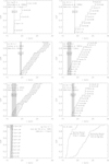 |
Fig. 2. Cumulative distribution function curves of the kHz QPO emission radius r, as well as the corresponding Sz values, for (a) Cyg X-2 (Sz ∼ − 0.09−1.13, r ∼ 17.4−21.5 km), (b) GX 5-1 (Sz ∼ 0.67−1.25, r ∼19.0−27.6 km), (c) GX 5-1 (Sz ∼ 0.12−1.10, r ∼ 19.3− 28.7 km), (d) GX 17+2 (Sz ∼ 0.08−1.45, r ∼ 16.6− 23.4 km), (e) GX 17+2 (Sz ∼ − 0.32−1.76, r ∼ 16.6−24.1 km), (f) GX 17+2 (Sz ∼ 0.16−1.16, r ∼ 18.0−24.0 km), and (g) Sco X-1 (Sz ∼ 1.25−2.09, r ∼ 16.1−17.0 km). The ranges of r that correspond to NB (Sz ∼ 1−2) are indicated in the shaded areas. (h) The CDF curves of all the kHz QPO emission radii that correspond to the HB (Sz ∼ − 0.32−0.97, r ∼ 17.4−28.7 km) and corresponds to the NB (Sz ∼ 1.01−2.09, r ∼ 16.1−19.9 km) by combining the r values in diagram (a) (Cyg X-2), (c) (GX 5-1), (e) (GX 17+2), and (g) (Sco X-1). |
4. Discussions and conclusions
Based on the Keplerian orbital motion assumption of the accretion plasma for the upper kHz QPOs, we investigated the evolution of the magnetosphere-disk radius r along the Z tracks of the luminous X-ray sources, Cyg X-2, GX 5-1, GX 17+2, and Sco X-1, and found that a radius range of r ∼ 16−29 km corresponds to the HB and NB branches. The details of the main results, together with the discussions and conclusions, are summarized as below:
– The magnetosphere-disk radius r inferred from the kHz QPOs of all the sources in Table 1 shows a monotonically decreasing trend (from r ∼ 28.7 km to r ∼ 16.1 km) from the HB to NB with increasing Sz values (from Sz ∼ −0.32 to Sz ∼ 2.09, see Figs. 2a–g, implying that the accretion disk moves toward the NS surface as the Z track evolves. It should be noticed that the evolution between these branches reflects the redistribution of the photons in the different energy bands. Take Cyg X-2 in Fig. 1a as an example. From the top to the bottom of the HB, the hard color (the ratio of the count rate in the bands of 9.8−15.9 keV/6.5−9.8 keV) decreases by ∼20% from ∼0.5 to ∼0.4, while the X-ray intensity (the 1.9−15.9 keV count rate) increases by a factor of ∼1.3 from ∼900 c s−1 to ∼1200 c s−1. Moreover, from the top to the bottom of the NB, the hard color decreases by ∼25% from ∼0.4 to ∼0.3 while the X-ray intensity decreases by ∼17% from ∼1200 c s−1 to ∼1000 c s−1. Therefore, we propose that as the accretion disk moves toward the NS surface, the dominated radiation components (e.g., thermal or nonthermal) may gradually change and cause the decrease of the hard color, then form the different branches.
– The magnetosphere-disk radii that correspond to the NBs of all the sources in Table 1 cluster around r ∼ 16−20 km, and are systematically smaller than those of the HBs with r ∼ 20−29 km (see Fig. 2h and Fig. 3). In addition, we note that the magnetosphere-disk radius that corresponds to the HB/NB vertex is found to be around r ∼ 20 km (see Figs. 2h and 3), implying a boundary that distinguishes the HB and NB. We suggest that the physical environment may dramatically change around this position, which causes the variation in the dominated radiation mechanism, where some kind of radiation phase transition may happen and result in the redistribution of the photons into the different energy bands. In addition, as this potential characteristic boundary around r ∼ 20 km is near the NS surface (the NS radius is R ∼ 15 km, see Miller & Miller 2015), so this radiation phase transition may relate to the physical environment around the NS surface, such as the hard NS surface and strong magnetic field.
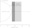 |
Fig. 3. Schematic diagram of the magnetosphere-disk structure of the Z source, where the shaded areas indicate the radius ranges that correspond to the HB (r ∼ 20−29 km) and the NB (r ∼ 16−20 km). |
– The inferred kHz QPO emission radii of Z sources share the range of r ∼ 16−30 km (see Table 1 and Fig. 2), which is similar to that of atoll sources based on the same Keplerian motion assumption (r ∼ 15−30 km, see Wang et al. 2017). The luminosity of Z sources is higher than that of atoll sources by about one to two orders of magnitude (van der Klis et al. 2006), and we prefer to consider that the Z sources share a higher accretion rate than the atoll sources. Generally, the disk accretion rate Ṁd can be expressed as (Shapiro & Teukolsky 1983)
 (3)
(3)
where 2h is the disk thickness, ρ is the mass density of the accretion plasma, and  is the fall velocity at the disk radius r. The atoll and Z sources share similar magnetosphere-disk radius ranges inferred from kHz QPOs, which can also suggest similar vr ranges. Then, we can infer from Eq. (3) that
  , where the Z sources with high Ṁd may share a thicker accretion disk than the atoll sources with low Ṁd. The disk thickness may affect the radiation process in NS-LMXBs. Firstly, the X-ray optical depth τ of the accretion disk is proportional to its geometric thickness, τ ∝ 2h (Shapiro & Teukolsky 1983), which implies that the thin and thick disks may share different optical depths. In addition, the motion of the charged particles in the strong magnetic field environment around the accretion disk can cause nonthermal radiation, however, these high energy photons may experience a Comptonization process due to the high optical depth when they transmit through the thick accretion disk. Secondly, the thicken of the accretion disk may also arise the radial accretion flow when the disk thickness is larger than the co-rotation radius of NS-LMXBs (i.e., h ≥ Rco), which will change the X-ray radiation components. Furthermore, the thin and thick accretion disks may share the different effects on the local magnetic field structure of NS. For instance, in the presence of the accretion disk, the NS magnetic field lines are “frozen-in” to the orbiting plasma, which are then sheared in the ϕ direction of the mid-plane disk (Shapiro & Teukolsky 1983; Bhattacharya & van den Heuvel 1991; Frank et al. 2002). These “frozen-in” magnetic field lines move inward with the accretion disk and pile up around the NS surface, which can induce the nondipole component and result in a local strong magnetic field region with
  and α ≥ 3 (Bs is the NS surface magnetic field strength). The more luminous Z sources with the thicker accretion disk may share more nondipole field components than the less luminous atoll sources, leading to a stronger interaction with the accretion plasma. Therefore, we propose that the atoll and Z behaviors may relate to the structures of both the accretion disk and the NS local magnetic field: the low luminosity atoll sources and high luminosity Z sources share the thin and thick accretion disks respectively, which cause the weak and strong effects on the NS local magnetic field, and these differences may induce the disparate X-ray radiation processes. In summary, the atoll and Z sources may exhibit a similar magnetosphere-disk radius range, but they share different accretions and local magnetic field environments that dominate the distinct X-ray radiation properties. This idea can also be applied to explain the transition between the atoll and Z behaviors of XTE J1701-462. This source shares the large scale magnetic field structure of a NS. When the source is in the low luminosity state, its exhibits a thin accretion disk and weak interaction with the NS local magnetic field, then it shows atoll-like behavior. While, when the source is in the high luminosity state, it exhibits a thick accretion disk and strong interaction with the NS local magnetic field, thus showing Z-like behavior. Moreover, as the magnetosphere-disk radii that correspond to the NBs of Z sources cluster around r ∼ 16−20 km, we suggest that the high magnetic energy density and high plasma mass density there may affect the radiation process and produce many soft photons.
As stressed, the conclusions obtained in this paper are based on certain theoretical assumptions. In fact, kHz QPO frequencies are directly detected in the observations, however, we are more interested in the physical process behind them. For one thing, most of the theoretical models propose that kHz QPOs originate from the matter motion in the inner accretion disk (van der Klis et al. 2006). For another, it is found that all the upper kHz QPOs detected in NS-LMXBs share frequencies larger than their corresponding NS spin frequencies, implying that ν2 should be involved in the Keplerian orbital frequency (Wang et al. 2018a). Thus, the upper kHz QPOs can be applied to explore the magnetosphere-disk radius with the Keplerian motion assumption. In addition, the magnetosphere-disk structure of NS-LMXBs inferred by kHz QPOs can trace out the physical environment around the accretion NS, such as the NS hard surface, the strong magnetic field, and their interaction with the accretion plasma, which can further be used to probe the X-ray radiation properties and the formation of the tracks in CCDs. Last but not least, it should also be said that our results on the evolution of the magnetosphere-disk structure along the Z track are based on different sources from various observations, so they should be common phenomena of Z sources that represent similar physical origins.
Acknowledgments
This work is supported by the National Natural Science Foundation of China (Grant No. 11703003, No. U1938117 and No. U1731238), the Guizhou Provincial Science and Technology Foundation (Grant No. [2020]1Y016).
References
- Abramowicz, M. A., Bulik, T., Bursa, M., & Kluźniak, W. 2003a, A&A, 404, L21 [NASA ADS] [CrossRef] [EDP Sciences] [Google Scholar]
- Abramowicz, M. A., Karas, V., Kluźniak, W., Lee, W. H., & Rebusco, P. 2003b, PASJ, 55, 467 [NASA ADS] [CrossRef] [Google Scholar]
- Altamirano, D., van der Klis, M., Meńdez, M., et al. 2008, ApJ, 685, 436 [NASA ADS] [CrossRef] [Google Scholar]
- Belloni, T., Psaltis, D., & van der Klis, M. 2002, ApJ, 572, 392 [NASA ADS] [CrossRef] [Google Scholar]
- Belloni, T., Méndez, M., & Homan, J. 2005, A&A, 437, 209 [NASA ADS] [CrossRef] [EDP Sciences] [Google Scholar]
- Belloni, T., Méndez, M., & Homan, J. 2007, MNRAS, 376, 1133 [NASA ADS] [CrossRef] [Google Scholar]
- Bhattacharya, D., & van den Heuvel, E. P. J. 1991, Phys. Rep., 203, 1 [NASA ADS] [CrossRef] [Google Scholar]
- Di Salvo, T., Méndez, M., van der Klis, M., Ford, E., & Robba, N. R. 2001, ApJ, 546, 1107 [NASA ADS] [CrossRef] [Google Scholar]
- Di Salvo, T., Méndez, M., & van der Klis, M. 2003, A&A, 406, 177 [NASA ADS] [CrossRef] [EDP Sciences] [Google Scholar]
- Ford, E. C., & van der Klis, M. 1998, ApJ, 506, L39 [NASA ADS] [CrossRef] [Google Scholar]
- Ford, E. C., van der Klis, M., Méndez, M., et al. 2000, ApJ, 537, 368 [NASA ADS] [CrossRef] [Google Scholar]
- Frank, J., King, A., & Raine, D. J. 2002, Accretion Power in Astrophysics, Third Ed. (Cambridge University Press) [Google Scholar]
- Fridriksson, J. K., Homan, J., & Remillard, R. A. 2015, ApJ, 809, 52 [NASA ADS] [CrossRef] [Google Scholar]
- Hasinger, G., & van der Klis, M. 1989, A&A, 225, 79 [NASA ADS] [Google Scholar]
- Hasinger, G., van der Klis, M., Ebisawa, K., Dotani, T., & Mitsuda, K. 1990, A&A, 235, 131 [NASA ADS] [Google Scholar]
- Hasinger, G. 1990, Rev. Mod. Astron., 3, 60 [NASA ADS] [CrossRef] [Google Scholar]
- Homan, J., van der Klis, M., Jonker, P. G., et al. 2002, ApJ, 568, 878 [NASA ADS] [CrossRef] [Google Scholar]
- Homan, J., van der Klis, M., Wijnands, R., et al. 2007, ApJ, 656, 420 [NASA ADS] [CrossRef] [Google Scholar]
- Homan, J., van der Klis, M., Fridriksson, J. K., et al. 2010, ApJ, 719, 201 [NASA ADS] [CrossRef] [Google Scholar]
- Jonker, P. G., Wijnands, R., van der Klis, M., et al. 1998, ApJ, 499, L191 [NASA ADS] [CrossRef] [Google Scholar]
- Jonker, P. G., van der Klis, M., Homan, J., et al. 2002, MNRAS, 333, 665 [NASA ADS] [CrossRef] [Google Scholar]
- Kaaret, P., Yu, W., Ford, E. C., & Zhang, S. N. 1998, ApJ, 497, L93 [NASA ADS] [CrossRef] [Google Scholar]
- Kluźniak, W. 2005, Astron. Nachr., 326, 820 [CrossRef] [Google Scholar]
- Kluźniak, W., Abramowicz, M. A., Kato, S., Lee, W. H., & Stergioulas, N. 2004, ApJ, 603, L89 [Google Scholar]
- Lamb, F. K., & Miller, M. C. 2001, ApJ, 554, 1210 [NASA ADS] [CrossRef] [Google Scholar]
- Lin, D. C., Remillard, R. A., & Homan, J. 2009, ApJ, 696, 1257 [NASA ADS] [CrossRef] [Google Scholar]
- Lin, D. C., Remillard, R. A., Homan, J., & Barret, D. 2012, ApJ, 756, 34 [NASA ADS] [CrossRef] [Google Scholar]
- Méndez, M. 2006, MNRAS, 371, 1925 [NASA ADS] [CrossRef] [Google Scholar]
- Méndez, M., & van der Klis, M. 1999, ApJ, 517, L51 [NASA ADS] [CrossRef] [Google Scholar]
- Méndez, M., & van der Klis, M. 2000, MNRAS, 318, 938 [NASA ADS] [CrossRef] [Google Scholar]
- Méndez, M., van der Klis, M., Ford, E. C., Wijnands, R., & van Paradijs, J. 1999, ApJ, 511, L49 [NASA ADS] [CrossRef] [Google Scholar]
- Méndez, M., van der Klis, M., & Ford, E. C. 2001, ApJ, 561, 1016 [NASA ADS] [CrossRef] [Google Scholar]
- Miller, M. C., & Miller, J. M. 2015, Phys. Rep., 548, 1 [NASA ADS] [CrossRef] [MathSciNet] [Google Scholar]
- Miller, M. C., Lamb, F. K., & Psaltis, D. 1998, ApJ, 508, 791 [NASA ADS] [CrossRef] [Google Scholar]
- Özel, F., & Freire, P. 2016, ARA&A, 54, 401 [Google Scholar]
- Psaltis, D., Belloni, T., & van der Klis, M. 1999, ApJ, 520, 262 [NASA ADS] [CrossRef] [Google Scholar]
- Ribeiro, E. M., Méndez, M., Zhang, G., & Sanna, A. 2017, MNRAS, 471, 1208 [CrossRef] [Google Scholar]
- Shapiro, S. L., & Teukolsky, S. A. 1983, Black Holes, White Dwarfs, and Neutron Stars: The Physics of Compact Objects (New York: Wiley Interscience) [Google Scholar]
- Stella, L., & Vietri, M. 1999, Phys. Rev. Lett., 82, 17 [NASA ADS] [CrossRef] [Google Scholar]
- Stella, L., Vietri, M., & Morsink, S. M. 1999, ApJ, 524, L63 [NASA ADS] [CrossRef] [Google Scholar]
- Török, G., Goluchová, K., Urbanec, M., et al. 2016, ApJ, 833, 273 [CrossRef] [Google Scholar]
- Török, G., Goluchová, K., Šrámková, E., Urbanec, M., & Straub, O. 2019, MNRAS, 488, 3896 [CrossRef] [Google Scholar]
- Troyer, J. S., Cackett, E. M., Peille, P., & Barret, D. 2018, ApJ, 860, 167 [CrossRef] [Google Scholar]
- van der Klis, M. 2000, ARA&A, 38, 717 [NASA ADS] [CrossRef] [Google Scholar]
- van der Klis, M. 2001, ApJ, 561, 943 [NASA ADS] [CrossRef] [Google Scholar]
- van der Klis, M. 2006, in Compact Stellar X-Ray Sources, eds. W. H. G. Lewin, & M. van der Klis (Cambridge: Cambridge Univ. Press), 39 [Google Scholar]
- van der Klis, M. 2016, Invited talk in European Week of Astronomy and Space Science, Timing Low-Mass X-Ray Binaries and Accreting Millisecond Pulsars, 4–8 July 2016, Athens, Greece [Google Scholar]
- van der Klis, M., Swank, J. H., Zhang, W., et al. 1996, ApJ, 469, L1 [NASA ADS] [CrossRef] [Google Scholar]
- van Doesburgh, M., & van der Klis, M. 2019, MNRAS, 490, 5270 [CrossRef] [Google Scholar]
- van Doesburgh, M., van der Klis, M., & Morsink, S. M. 2018, MNRAS, 479, 426 [CrossRef] [Google Scholar]
- van Straaten, S., Ford, E. C., van der Klis, M., Méndez, M., & Kaaret, P. 2000, ApJ, 540, 1049 [NASA ADS] [CrossRef] [Google Scholar]
- van Straaten, S., van der Klis, M., & Méndez, M. 2003, ApJ, 596, 1155 [NASA ADS] [CrossRef] [Google Scholar]
- Wang, D. H., Chen, L., Zhang, C. M., & Qu, J. L. 2014, Astron. Nachr., 335, 168 [NASA ADS] [CrossRef] [Google Scholar]
- Wang, D. H., Zhang, C. M., Lei, Y. J., et al. 2017, MNRAS, 1111, 1117 [Google Scholar]
- Wang, D. H., Zhang, C. M., Qu, J. L., & Yang, Y. Y. 2018a, MNRAS, 473, 4862 [NASA ADS] [CrossRef] [Google Scholar]
- Wang, D. H., Zhang, C. M., & Qu, J. L. 2018b, A&A, 618, A181 [CrossRef] [EDP Sciences] [Google Scholar]
- Wijnands, R., Homan, J., van der Klis, M., et al. 1997a, ApJ, 490, L157 [NASA ADS] [CrossRef] [Google Scholar]
- Wijnands, R. A. D., van der Klis, M., Kuulkers, E., Asai, K., & Hasinger, G. 1997b, A&A, 323, 399 [Google Scholar]
- Wijnands, R., Homan, J., van der Klis, M., et al. 1998a, ApJ, 493, L87 [NASA ADS] [CrossRef] [Google Scholar]
- Wijnands, R., Meńdez, M., van der Klis, M., et al. 1998b, ApJ, 504, L35 [NASA ADS] [CrossRef] [Google Scholar]
- Zhang, C. M. 2004, A&A, 423, 401 [NASA ADS] [CrossRef] [EDP Sciences] [Google Scholar]
- Zhang, C. M., & Wang, D. H. 2013, in Feeding Compact Objects: Accretion on All Scales, eds. C. M. Zhang, T. Belloni, M. Mendez, et al. (Cambridge: Cambridge University Press), Proc. IAU Symp., 290, 381 [Google Scholar]
- Zhang, C. M., Yin, H. X., Zhao, Y. H., Zhang, F., & Song, L. M. 2006, MNRAS, 366, 1373 [NASA ADS] [CrossRef] [Google Scholar]
- Zhang, C. M., Wang, J., Zhao, Y. H., et al. 2011, A&A, 527, A83 [NASA ADS] [CrossRef] [EDP Sciences] [Google Scholar]
- Zhang, G., Méndez, M., Sanna, A., Ribeiro, E. M., & Gelfand, J. D. 2017, MNRAS, 465, 5003 [CrossRef] [Google Scholar]
All Tables
All Figures
|
Fig. 1. Schematic diagrams of the Z tracks in the hardness-intensity diagrams, for (a) Cyg X-2, (b) GX 5-1, (c) GX 17+2, and (d) Sco X-1, where the approximate positions of the HB/NB vertex (Sz ∼ 1) and NB/FB vertex (Sz ∼ 2) are indicated by the parameter Sz as defined by Hasinger et al. (1990) and Wijnands et al. (1997b) (see the text). On the axis quantities of the diagrams, the hard colors are defined as the ratio of the count rate in the bands of 9.8−15.9 keV/6.5−9.8 keV for Cyg X-2, GX 5-1, and GX 17+2, and 9.8−15.9 keV/6.4−9.8 keV for Sco X-1, while the X-ray intensities are defined as the count rate in 1.9−15.9 keV for Cyg X-2, GX 5-1, GX 17, and 2.0−15.9 keV for Sco X-1. The diagrams are produced with the same RXTE data as that in Wijnands et al. (1998a) for Cyg X-2, Jonker et al. (2002) for GX 5-1, Homan et al. (2002) for GX 17+2, and van der Klis et al. (1996) for Sco X-1. The hard colors are not dead-time corrected because of the small correction factors (< 0.2%). |
| In the text | |
|
Fig. 2. Cumulative distribution function curves of the kHz QPO emission radius r, as well as the corresponding Sz values, for (a) Cyg X-2 (Sz ∼ − 0.09−1.13, r ∼ 17.4−21.5 km), (b) GX 5-1 (Sz ∼ 0.67−1.25, r ∼19.0−27.6 km), (c) GX 5-1 (Sz ∼ 0.12−1.10, r ∼ 19.3− 28.7 km), (d) GX 17+2 (Sz ∼ 0.08−1.45, r ∼ 16.6− 23.4 km), (e) GX 17+2 (Sz ∼ − 0.32−1.76, r ∼ 16.6−24.1 km), (f) GX 17+2 (Sz ∼ 0.16−1.16, r ∼ 18.0−24.0 km), and (g) Sco X-1 (Sz ∼ 1.25−2.09, r ∼ 16.1−17.0 km). The ranges of r that correspond to NB (Sz ∼ 1−2) are indicated in the shaded areas. (h) The CDF curves of all the kHz QPO emission radii that correspond to the HB (Sz ∼ − 0.32−0.97, r ∼ 17.4−28.7 km) and corresponds to the NB (Sz ∼ 1.01−2.09, r ∼ 16.1−19.9 km) by combining the r values in diagram (a) (Cyg X-2), (c) (GX 5-1), (e) (GX 17+2), and (g) (Sco X-1). |
| In the text | |
|
Fig. 3. Schematic diagram of the magnetosphere-disk structure of the Z source, where the shaded areas indicate the radius ranges that correspond to the HB (r ∼ 20−29 km) and the NB (r ∼ 16−20 km). |
| In the text | |
Current usage metrics show cumulative count of Article Views (full-text article views including HTML views, PDF and ePub downloads, according to the available data) and Abstracts Views on Vision4Press platform.
Data correspond to usage on the plateform after 2015. The current usage metrics is available 48-96 hours after online publication and is updated daily on week days.
Initial download of the metrics may take a while.