| Issue |
A&A
Volume 641, September 2020
|
|
|---|---|---|
| Article Number | A21 | |
| Number of page(s) | 5 | |
| Section | The Sun and the Heliosphere | |
| DOI | https://doi.org/10.1051/0004-6361/202038182 | |
| Published online | 01 September 2020 | |
A new method for estimating global coronal wave properties based on their interaction with solar coronal holes
1
Departament de Física, Universitat de les Illes Balears (UIB), 07122 Palma, Spain
e-mail: isabell.piantschitsch@uib.es
2
Institute of Applied Computing & Community Code (IAC 3), UIB, Palma, Spain
3
Institute of Physics, University of Graz, Universitätsplatz 5, 8010 Graz, Austria
Received:
16
April
2020
Accepted:
15
June
2020
Among the effects of interactions between global coronal waves (CWs) and coronal holes (CHs) is the formation of reflected and transmitted waves. Observations of such events provide us with measurements of different CW parameters, such as phase speed and intensity amplitudes. However, several of these parameters are provided with only intermediate observational quality, whereas other parameters, such as the phase speed of transmitted waves, can hardly be observed in general. We present a new method to estimate crucial CW parameters, such as density and phase speed of reflected as well as transmitted waves, Mach numbers and density values of the CH’s interior, by using analytical expressions in combination with the most basic and most accessible observational measurements available. The transmission and reflection coefficients were derived from linear theory and used to calculate estimations for phase speeds of incoming, reflected, and transmitted waves. The obtained analytical expressions were validated by performing numerical simulations of CWs interacting with CHs. This new method enables us to determine in a fast and straightforward way reliable CW and CH parameters from basic observational measurements which provides a powerful tool to better understand the observed interaction effects between CWs and CHs.
Key words: magnetohydrodynamics (MHD) / waves / Sun: magnetic fields
© ESO 2020
1. Introduction
Coronal waves (CWs) are large-scale propagating disturbances in the corona which are considered to be fast mode magnetohydrodynamic (MHD) waves (see e.g. Vršnak & Lulić 2000). Evidence for their wave characteristics is given from observations of secondary waves interacting with coronal holes (CHs), representing regions of sudden changes in density, Alfvén, and magnetosonic speed. Secondary waves are caused by reflection and refraction at the boundary of a CH (e.g. Kienreich et al. 2013; Long et al. 2008; Gopalswamy et al. 2009) or transmission through a CH (Olmedo et al. 2012; Liu et al. 2019). Case studies of chromospheric Moreton waves also show a partial penetration into a CH (e.g. Veronig et al. 2006). Numerical simulations confirm the wave interpretation in accordance with the observations by finding effects such as deflection, reflection, and refraction when the wave interacts with such a structure as a CH (Afanasyev & Zhukov 2018; Piantschitsch et al. 2018a,b).
Typical wave parameters of primary and secondary wave fronts that can be measured using observations are phase speed, intensity amplitude, and width (e.g. Muhr et al. 2011; Kienreich et al. 2011). However, secondary and, in particular, transmitted waves are rather weak in their signal, hence, quality, and accuracy of measurements are rather low which might lead to a misinterpretation of the results. This is based on the fact that other coronal parameters that provide information, for example, about the CH itself are difficult to derive. In particular, information about the dynamics and density distribution inside of a CH is mostly unavailable due to the CH’s low density compared to the surrounding area. Numerical simulations are capable of providing additional information about CW parameters and the interaction effects between CWs and CHs, but are still limited considering their necessary idealisation and dependence on initial conditions.
The aim of this paper is, therefore, to establish a method for determining estimations for important CW parameters, such as the density amplitudes of reflected and transmitted waves by using simple analytical terms in combination with basic observational measurements. These estimations will be obtained by first analytically deriving reflection and transmission coefficients from linear theory and, second, complementing these terms with simple expressions of nonlinear MHD waves. We aim to validate the theoretical expressions by performing numerical simulations of CW propagation and its interaction with CHs. For the comparison of the theoretical results with the observations, we chose two different events detailing a CW-CH-interaction, which differ in their phase speed of the secondary waves. The first case represents a purely acoustic case where the phase speed is close to the typical sound speed (Kienreich et al. 2013). The other case will be used to validate the theoretical expressions determined for the purely magnetic case due to the fact that the observed phase speed of the incoming wave is close to 700 km s−1 (Olmedo et al. 2012). Overall, we will show that this newly developed method is a useful and fast tool for providing important information about CW parameters and dynamics inside a CH, as well as the interaction effects between CWs and CHs.
2. Theoretical results
In this section, we first analytically derive the reflection and transmission coefficients from linear theory and validate these terms by performing numerical simulations of CW-CH-interaction. Secondly, we use these coefficients to obtain analytical expressions for the phase speeds of incoming, reflected, and transmitted waves.
2.1. Linear case
We start with a simple equilibrium based on uniform density, ρ0, gas pressure, p0, and a magnetic field, B0, pointing in the z-direction. We focus on perturbations propagating in the x-direction perpendicularly to the magnetic field and representing CWs. Since the equilibrium is homogeneous, sound ( ) and Alfvén speeds (
 ) are constant, and fluctuations in the system propagate as plane waves. For the velocity, we have
By using this expression in the standard linearised MHD equations and performing the temporal and spatial derivatives, a dispersion relation is readily obtained
which corresponds to fast MHD waves propagating purely perpendicular to the magnetic field at the fast speed (cf0). The density changes due to these waves in the linear regime are given by the simple expression
for right (+) and left (−) propagating waves.
In the low-β situation, we neglect the sound speed since it is negligibly small compared to the Alfvén speed and the dispersion relation reduces to ω = kx vA0. In the high-β limit, the magnetic field is very weak and we obtain the dispersion relation of purely acoustic waves, ω = kx cs0.
We then extend the situation for a homogeneous medium to the interface problem which is based on two different homogeneous media connected through a discontinuity at x = 0 (with densities ρ01 in region 1 and ρ02 in region 2; see top panel in Fig. 1). This is an idealised representation of a CH (corresponding to region 2 with ρ02 < ρ01) but allows us to consider the basic properties of the reflection and transmission of a fast MHD wave at a density step.
 |
Fig. 1. Density (top panel) and velocity (bottom panel) at five different times during the evolution of a linear (solid line) and weakly nonlinear (dashed line) perturbation representing an idealised CW. The incoming wave (red) steepens into a shock in the nonlinear regime. The reflected wave at the interface between region 1 and region 2, which represents the CH boundary (located at x = 0) is a rarefaction wave (black) while the transmitted (blue) is a shock wave. |
We assume again a plane wave propagating in region 1, which interacts with the interface and generates a reflected wave at the CH boundary (x = 0). The incoming and reflected waves at the interface are of the form

In region 2, there is a transmitted wave traveling through the CH,
In this problem, the frequency, ω, is constant but the wave number changes according to the dispersion relation in the corresponding medium. For this reason we have now two wavenumbers, kx1 and kx2. Again, if the sound speed is negligible compared to the Alfvén speed we obtain kx1 = ω/vA01 and kx2 = ω/vA02. The amplitudes of the velocities in the two regions are not independent from each other since the variables have to satisfy certain conditions at the interface (see, for example, Walker 2004). In particular, the velocity and the total pressure have to be continuous at x = 0 (the location of the interface). When these conditions are fulfilled it is straight forward to obtain the following amplitudes
which correspond to the reflection coefficient as a function of the incoming wave amplitude, v0, and
for the transmission coefficient, where the density contrast is defined as  (0 < ξ < 1 for CHs). We note that the coefficients satisfy the equation v0 + vR = vT and always carry the sign of v0.
We can assume that the velocity amplitude of the incoming wave, v0, is positive. This means that, according to Eq. (3), the incoming wave has a density enhancement associated to it (ρ > ρ0). On the contrary, the reflected wave, with a negative sign in Eq. (3) but being vR > 0 (because v0 > 0, see Eq. (6)) corresponds to a density dimming (ρ < ρ0). This is in agreement with the reported reflections of CWs at CHs by most of the observations (e.g. Kienreich et al. 2013; Gopalswamy et al. 2009).
Finally, it turns out that for pure sound waves, the reflection and transmission coefficients are exactly the same as for the purely magnetic case, therefore Eqs. (6) and (7) are used in the acoustic case as well. In this last situation, the linear density fluctuations are given by Eq. (3) but with cf0 replaced by cs0.
2.2. Numerical experiments in the linear regime
Now the MHD wave propagation and its interaction with a region of lower density such as a CH is solved numerically by using the standard ideal MHD equations (see Piantschitsch et al. 2017, 2018a,b, for details). An initial Gaussian linear perturbation is introduced into the system and the evolution of this fluctuation is followed in time, see Fig. 1. This Gaussian pulse can be interpreted as a superposition and combination of different plane harmonic waves, therefore, the linear analysis performed in Sect. 2.1 can be applied to these simulations. The incident wave, corresponding to a density enhancement (solid red lines in the top panel) travels toward the right and eventually interacts with the density discontinuity at x = 0. A reflected density dimming, with a low amplitude, then travels to the left (solid black line), while a density enhancement is moving at a faster speed towards the right inside the CH (solid blue line). Similar results are found for the velocities, see solid lines in the lower panel of Fig. 1. These are the expected results from linear theory. From the simulations we are able to derive the reflected and transmitted velocity amplitudes, see the circles in Fig. 2, and compare them to the analytical expressions for the reflection and transmission coefficents which we derived in Sect. 2.1 The values obtained from the simulations show good agreement with the theoretical calculations in the linear regime (v0 ≪ vA01).
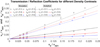 |
Fig. 2. Transmitted (circles) and reflected velocity amplitudes (diamonds) as a function of the incident velocity amplitude (v0) inferred from the linear and nonlinear MHD simulations for different density contrasts. The dashed and solid lines correspond to the predicted analytical results using the transmission and reflection coefficients given by Eqs. (7) and (6). |
2.3. Nonlinear case
There is evidence that CWs which are propagating in the corona and interacting with CHs are of nonlinear nature (Vršnak & Lulić 2000; Warmuth et al. 2004). For pure sound waves (vA0 = 0), the nonlinear results are well known and can be found, for example, in Mihalas & Mihalas (1984), Landau & Lifshitz (1987). The nonlinear wave with a velocity amplitude, v, modifies the local sound speed, cs, which is now different from the unperturbed reference sound velocity, cs0. For the phase speed of the nonlinear wave, we obtain vp(v) = v ± cs and it can be shown that it is reduced to the simple expression
where we have again the distinction between right and left propagating waves. The dependence of the phase velocity of the wave on v leads to the steepening of the wave. Then density variations in the nonlinear wave are related to velocity through the following equation under adiabatic conditions,
For the purely magnetic fast wave (cs0 = 0), it is a straightforward exercise to derive equivalent equations by exchanging the adiabatic condition with the magnetic induction equation. It can be shown that in this case and for perpendicular propagation (see some details in Mann 1995) the phase speed is vp(v) = v ± vA. Again, it is not difficult to show that this expression is reduced to
This equation is rather simple since we have eliminated the Alfvén speed modified by the presence of the wave (vA), and it involves only the unperturbed Alfvén speed (vA0) and the velocity amplitude of the wave (v). It can be shown that at this point, density variations in the wave are related to velocity through the following equation
In the limit v/vA0 ≪ 1, this expression leads to the linear result of Eq. (3). As noted by Mann (1995) the expressions for the magnetic case are simply obtained by setting γ = 2 and replacing cs0 by vA0 in the equations for the nonlinear acoustic case. When acoustic and magnetic effects are combined, the problem is more difficult and it requires a numerical treatment which is beyond the scope of this paper.
2.4. Numerical experiments in the nonlinear regime
Here we extend the results of Sect. 2.2 to the nonlinear situation. The amplitude of the initial Gaussian perturbation is increased, meaning that the velocity of the wave just before it interacts with the CH (v0 in our notation) is larger than in the linear case. Now the wave shows some steepening as it is approaching the CH (see Fig. 1, red dashed line in region 1 of the lower panel) and also once it is transmitted through the CH (blue dashed line). The velocity amplitude of the wave is larger inside the CH and the width of the pulse has increased. The behaviour of the signal in each region follows the behaviour predicted in Sect. 2.3 and the equations for the density as a function of velocity are exact. But more importantly, even beyond the linear regime, there is still a good agreement with the reflection and transmission amplitudes based on the linear calculations; see circles in Fig. 2 for v0/vA01 > 0.1. In this figure, we can see that for a density contrast of  the transmitted amplitude agrees quite well with the predicted linear value (see dashed blue line). The differences become more prominent the smaller the density contrast, however, in the worst case the error is only around 12%. This has important consequences for the method developed in this work, meaning that the simple linear expressions for reflection and transmission coefficients can be used to estimate vital CW parameters which are originally nonlinear in nature.
2.5. Implications
The measured phase speed of the incoming front in the observations is denoted by uI, while the measured reflected phase velocity is uR. According to the previous equations for the purely magnetic case, we have (see Eq. (10)) for the incoming wave
while for the reflected wave (we implicitly assume that it is propagating to the left and the global minus sign is not taken into account)
By combining Eqs. (12) and (13) we obtain
We note that vR and vT are simply the reflected and transmitted amplitudes given by Eqs. (6) and (7). Although we are dealing with nonlinear waves, the linear results about the reflection and transmission problem are still applicable (this is a key point of the method presented here; see Sect. 2.4). We do not need to apply the Rankine-Hugoniot jump conditions.
3. Application to observations
In this section, we apply the analytical expressions we obtained in Sect. 2 to the observations and compare the results to two different case studies which differ in the phase speed measurements of the propagating CW.
It is a straightforward task to use the transmitted amplitude in Eq. (14) to obtain the velocity amplitude of the incoming wave in terms of the density contrast,  , and the phase velocities of incident and reflected waves,
Therefore, we are able to calculate the velocity amplitude of the front close to the CH boundary, a magnitude that the observations are unlikely to provide. With this information and by using Eq. (12), the local Alfvén speed is simply
Repeating the same derivation but for the purely acoustic case we now find that
while the background sound speed is given by
which is completely equivalent to Eq. (16) for fast purely magnetic waves. We note that since the density contrast satisfies 0 < ξ < 1, we always have that uR < cs01 < uI and the same applies to vA01.
Another important variable that is computed, once we know v0, is the density enhancement and dimming associated to the incoming, reflected, and transmitted wave. From Eq. (9), we have for the incoming wave:

while for the dimming due to the reflection
where we have again used the expression for the reflection coefficient. The enhancement of the transmitted wave is
The expressions for the density fluctuations in the case of the magnetic case are given by Eqs. (19)–(21) but making the substitution γ = 2 (instead of using 5/3).
Finally, we derive an expression for the phase velocity of the transmitted wave into the CH in terms of the phase velocities of the incoming and reflected waves,
This expression is the same for the purely magnetic case and for the purely acoustic case and we have used the fact that in our model, vA02 = vA01/ξ and cs02 = cs01/ξ. If measurements of incoming, reflected, and transmitted phase speeds can be provided, we are able to calculate the density contrast by using Eq. (22). If, in addition, density measurements of the quiet Sun can be obtained from observations, we may even be capable of estimating the density inside of the CH.
In the following, we apply actually measured values of incoming and reflected phase speeds (uI, uR), as well as measured density contrasts inside and outside the CH (ρ02/ρ01) in order to calculate the CW parameters, v0, vA01 or cs01, ρI, ρR, ρT, and uT, by using the previous equations.
3.1. Event 1
Kienreich et al. (2013) analysed three homologous wave events referred to as W1, W2, and W3 in Tables 1 and 2, with clear reflection effects due to interaction with the same CH. The incident angle of the wave with respect to the CH normal is ≈10°, meaning that the wave propagates almost perpendicularly to the CH boundary which is in agreement with the theoretical assumption made in Sect. 2. Incoming phase speeds and errors for the three primary waves are derived with uI = [155 ± 17, 180 ± 18, 219 ± 15] km s−1, while for the corresponding reflected waves, the phase speeds are found to be uR = [119 ± 28, 164 ± 33, 198 ± 34] km s−1 (Kienreich et al. 2013). Since the phase speeds are close to the typical sound speed for a 1 MK corona, we test the interpretation in terms of purely acoustic waves.
Calculated values for velocity amplitude of the incoming wave, sound speed, Alfvén speed, Mach number (M) and phase speed of the transmitted wave for Events 1 and 2.
Calculated values for density enhancement/dimming associated to incoming, reflected and transmitted wave for Events 1 and 2.
For the calculations, we use a density contrast of  and an error of ±0.02, which has been derived from the density ratios using 193 and 195 Å EUV image data in Event 1 and Event 2 (considering
  ; see Zhukov 2011). The corresponding errors are calculated using the standard error-propagation formula. For the phase velocities, we use the values given by the observations in Event 1 and Event 2. The calculated values for the velocities using Eqs. (15)–(18), the corresponding Mach numbers and the transmitted phase speeds are found in Table 1. The acoustic and Alfvénic Mach numbers (M) are defined as the ratio of the velocity amplitude of the incoming wave to the sound speed and the Alfvén speed, respectively. The values for the densities calculated using Eqs. (19)–(21) are shown in Table 2. The estimated errors are also included in the tables.
3.2. Event 2
Olmedo et al. (2012) also reported coronal waves reflected at a CH, which were not, however, caused by a strictly perpendicular incoming wave as the shape of the CH is rather complex. However, we chose this event since it is one of the most well-known cases for CW-CH-interaction, additionally providing measurements for the transmitted wave, which are generally lacking in the literature. The phase speed of the incident wave in this event is around 720 ± 20 km s−1, while the reflected wave propagates at 280 ± 10 km s−1. In this case, the phase speed is closer to typical Alfvén speed values rather than to the sound speed; it is for this reason that we give the estimation based on the magnetic interpretation only. Olmedo et al. (2012) also found variations in the speed of the reflected wave, which shows that there might be projection effects and variations of the local speed. Secondary waves are reported to be deflected into the higher corona, which could also lead to a smaller projected speed (see Kienreich et al. 2013). The obtained values for the CW parameters are found in Tables 1 and 2 (see Event 2).
From statistical studies, we know that the density ratio lies between 0.1 and 0.6 (e.g. Saqri et al. 2020; Heinemann et al. 2019). If we assume  , then we are able to calculate upper and lower limits for the different parameters by using Eqs. (15)–(22) and the limits for the density contrast. For example, for Wave 1 in Event 1, we obtain 18 ≤ v0 ≤ 23, 123 ≤ vA0 ≤ 131, 0.14 ≤ M ≤ 0.19, 212 ≤ uT ≤ 451, 1.14 ≤ ρI/ρ01 ≤ 1.20, 0.93 ≤ ρR/ρ01 ≤ 0.97, and 1.22 ≤ ρT/ρ02 ≤ 1.23. Analogously, parameter limits, and therefore the dependence on the density contrast ξ, can be obtained for the other waves in both events.
4. Discussion and conclusions
We present a new and reliable method for calculating coronal wave parameters by using analytical expressions derived from linear wave theory and augmented by simple nonlinear terms of fast-mode MHD waves. The results were validated by performing numerical simulations of CW-CH-interaction and applied to two different observational cases. With this, we clearly emphasise the powerful combination between theory, simulations, and observations.
The main results are summarised as follows:
-
We applied the theoretical estimations to observations by calculating coronal wave parameters (e.g. density amplitudes, transmitted phase speed) by using incoming and reflected phase speeds and density contrast from the observations (see Eqs. (19)–(22)).
-
We performed numerical simulations of CW-CH-interactions and compared the results to the analytically and linear theory-derived reflection and transmission coefficients (see Eqs. (6) and (7)). The obtained values show good agreement for the linear as well as the weakly nonlinear case, validating the method proposed in this paper (see Fig. 2).
-
Moreover, if measurements of incoming, reflected, and transmitted phase speeds are provided, the analytical expressions derived in this work can be used to obtain information about the CH itself, such as the density inside the CH and the density contrast to the surrounding area (see Eq. (22)).
-
Using the derived expressions for the local sound and Alfvén speeds (see Eqs. (16) and (18)), we are able to calculate the Mach numbers associated with the waves (see Table 1). The large errors for these values can be explained by the uncertainties in the observed phase velocities.
-
Assuming we know the density contrast of the CH and its surroundings, we are also able to calculate the Alfvén speed and the Mach number inside the CH.
-
If we know the density of the region of the incoming wave, we are able to calculate the value of the magnetic field using the inferred Alfvén speed.
We have to keep in mind that what we are considering is a simplified model of the actual situation in the observations. Specifically, we studied a front that is perpendicular to the interface, which is not necessarily true in a real situation. The effect of the incident angle of the front needs to be taken into account in future studies. However, we have shown that theoretical estimations that were mainly derived from linear theory are a useful tool for calculating important coronal wave parameters in a quick and straightforward way, allowing us to proceed to performing coronal seismology studies.
Acknowledgments
We thank the anonymous referee for careful consideration of this manuscript and helpful comments. I.P. and J.T. acknowledge the support from grant AYA2017-85465-P (MINECO/AEI/FEDER, UE), to the Conselleria d’Innovació, Recerca i Turisme del Govern Balear, and also to IAC3. This work was supported by the Austrian Science Fund (FWF): I 3955-N27.
References
- Afanasyev, A. N., & Zhukov, A. N. 2018, A&A, 614, A139 [NASA ADS] [CrossRef] [EDP Sciences] [Google Scholar]
- Gopalswamy, N., Yashiro, S., Temmer, M., et al. 2009, ApJ, 691, L123 [NASA ADS] [CrossRef] [Google Scholar]
- Heinemann, S. G., Temmer, M., Heinemann, N., et al. 2019, Sol. Phys., 294, 144 [CrossRef] [Google Scholar]
- Kienreich, I. W., Veronig, A. M., Muhr, N., et al. 2011, ApJ, 727, L43 [Google Scholar]
- Kienreich, I. W., Muhr, N., Veronig, A. M., et al. 2013, Sol. Phys., 286, 201 [NASA ADS] [CrossRef] [Google Scholar]
- Landau, L. D., & Lifshitz, E. M. 1987, Fluid Mechanics (Oxford: Pergamon Press) [Google Scholar]
- Liu, R., Wang, Y., Lee, J., & Shen, C. 2019, ApJ, 870, 15 [Google Scholar]
- Long, D. M., Gallagher, P. T., McAteer, R. T. J., & Bloomfield, D. S. 2008, ApJ, 680, L81 [Google Scholar]
- Mann, G. 1995, J. Plasma Phys., 53, 109 [NASA ADS] [CrossRef] [Google Scholar]
- Mihalas, D., & Mihalas, B. W. 1984, Foundations of Radiation Hydrodynamics (New York: Oxford University Press) [Google Scholar]
- Muhr, N., Veronig, A. M., Kienreich, I. W., Temmer, M., & Vršnak, B. 2011, ApJ, 739, 89 [Google Scholar]
- Olmedo, O., Vourlidas, A., Zhang, J., & Cheng, X. 2012, ApJ, 756, 143 [NASA ADS] [CrossRef] [Google Scholar]
- Piantschitsch, I., Vršnak, B., Hanslmeier, A., et al. 2017, ApJ, 850, 88 [Google Scholar]
- Piantschitsch, I., Vršnak, B., Hanslmeier, A., et al. 2018a, ApJ, 857, 130 [Google Scholar]
- Piantschitsch, I., Vršnak, B., Hanslmeier, A., et al. 2018b, ApJ, 860, 24 [Google Scholar]
- Saqri, J., Veronig, A. M., Heinemann, S. G., et al. 2020, Sol. Phys., 295, 6 [Google Scholar]
- Veronig, A. M., Temmer, M., Vršnak, B., & Thalmann, J. K. 2006, ApJ, 647, 1466 [NASA ADS] [CrossRef] [EDP Sciences] [Google Scholar]
- Vršnak, B., & Lulić, S. 2000, Sol. Phys., 196, 157 [Google Scholar]
- Walker, A. 2004, in Magnetohydrodynamic Waves in Geospace, Ser. Plasma Phys., 16 [Google Scholar]
- Warmuth, A., Vršnak, B., Magdalenić, J., Hanslmeier, A., & Otruba, W. 2004, A&A, 418, 1101 [NASA ADS] [CrossRef] [EDP Sciences] [Google Scholar]
- Zhukov, A. N. 2011, J. Atmos. Solar-Terr. Phys., 73, 1096 [Google Scholar]
All Tables
Calculated values for velocity amplitude of the incoming wave, sound speed, Alfvén speed, Mach number (M) and phase speed of the transmitted wave for Events 1 and 2.
Calculated values for density enhancement/dimming associated to incoming, reflected and transmitted wave for Events 1 and 2.
All Figures
|
Fig. 1. Density (top panel) and velocity (bottom panel) at five different times during the evolution of a linear (solid line) and weakly nonlinear (dashed line) perturbation representing an idealised CW. The incoming wave (red) steepens into a shock in the nonlinear regime. The reflected wave at the interface between region 1 and region 2, which represents the CH boundary (located at x = 0) is a rarefaction wave (black) while the transmitted (blue) is a shock wave. |
| In the text | |
|
Fig. 2. Transmitted (circles) and reflected velocity amplitudes (diamonds) as a function of the incident velocity amplitude (v0) inferred from the linear and nonlinear MHD simulations for different density contrasts. The dashed and solid lines correspond to the predicted analytical results using the transmission and reflection coefficients given by Eqs. (7) and (6). |
| In the text | |
Current usage metrics show cumulative count of Article Views (full-text article views including HTML views, PDF and ePub downloads, according to the available data) and Abstracts Views on Vision4Press platform.
Data correspond to usage on the plateform after 2015. The current usage metrics is available 48-96 hours after online publication and is updated daily on week days.
Initial download of the metrics may take a while.