| Issue |
A&A
Volume 640, August 2020
|
|
|---|---|---|
| Article Number | A121 | |
| Number of page(s) | 16 | |
| Section | Planets and planetary systems | |
| DOI | https://doi.org/10.1051/0004-6361/202037569 | |
| Published online | 26 August 2020 | |
Colors of an Earth-like exoplanet
Temporal flux and polarization signals of the Earth
1
Faculty of Aerospace Engineering, Delft University of Technology,
Delft, The Netherlands
e-mail: This email address is being protected from spambots. You need JavaScript enabled to view it.
2
LATMOS/IPSL, UVSQ Université Paris-Saclay, Sorbonne Université, CNRS,
Guyancourt,
France
Received:
24
January
2020
Accepted:
12
June
2020
Abstract
Context. Understanding the total flux and polarization signals of Earth-like planets and their spectral and temporal variability is essential for the future characterization of such exoplanets.
Aims. We provide computed total (F) and linearly (Q and U) and circularly (V) polarized fluxes, and the degree of polarization P of sunlight that is reflected by a model Earth, to be used for instrument designs, optimizing observational strategies, and/or developing retrieval algorithms.
Methods. We modeled a realistic Earth-like planet using one year of daily Earth-observation data: cloud parameters (distribution, optical thickness, top pressure, and particle effective radius), and surface parameters (distribution, surface type, and albedo). The Stokes vector of the disk-averaged reflected sunlight was computed for phase angles α from 0° to 180°, and for wavelengths λ from 350 to 865 nm.
Results. The total flux F is one order of magnitude higher than the polarized flux Q, and Q is two and four orders of magnitude higher than U and V, respectively. Without clouds, the peak-to-peak daily variations due to the planetary rotation increase with increasing λ for F, Q, and P, while they decrease for U and V. Clouds modify but do not completely suppress the variations that are due to rotating surface features. With clouds, the variation in F increases with increasing λ, while in Q, it decreases with increasing λ, except at the largest phase angles. In earlier work, it was shown that with oceans, Q changes color from blue through white to red. The α where the color changes increases with increasing cloud coverage. Here, we show that this unique color change in Q also occurs when the oceans are partly replaced by continents, with or without clouds. The degree of polarization P shows a similar color change. Our computed fluxes and degree of polarization will be made publicly available.
Key words: radiative transfer / polarization / techniques: polarimetric / planets and satellites: terrestrial planets / planets and satellites: atmospheres / planets and satellites: surfaces
Now at Royal Netherlands Meteorological Institute (KNMI), De Bilt, The Netherlands.
© ESO 2020
1 Introduction
Since the discovery of 51 Pegasi b (Mayor & Queloz 1995), several thousand exoplanets have been discovered and confirmed1, including various Earth-sized planets in the habitable zones around their parent stars (Chou et al. 2017). A recent addition to the latter selection is TOI-700b, an Earth-sized planet in the habitable zone of red dwarf star TOI-700, as discovered by Gilbert et al. (2020) and confirmed with Spitzer observations by Rodriguez et al. (2020).
The planetary physical properties that can be derived from measurements with the two most successful exoplanet detection techniques, that is, with the radial velocity method and the transit method, are the planet radius (if the planet transits its star), mass (a lower limit if the planet does not transit its star), and the orbital period and distance, eccentricity, and inclination (if the planet transits its star) (see Perryman 2018, and references therein). The upper atmospheres (above optically thick clouds) of giant exoplanets and those of smaller planets around M stars can be probed using spectroscopy during primary and/or secondary transits (Bean et al. 2010; Swain et al. 2009, 2008; Tinetti et al. 2007; Nakajima 1983). It appears to be virtually impossible to characterize the (lower) atmospheresand surfaces of small, Earth-like planets in the habitable zones of solar-type stars (Bétrémieux & Kaltenegger 2014; Misra et al. 2014; Kaltenegger & Traub 2009), in particular because the light of the parent star is refracted while traveling through the lower atmosphere of its planet and emerges forever out of reach of terrestrial telescopes (García Muñoz et al. 2012). The (lower) atmosphere and surface of a planet are crucial for determining the habitability of a planet, as they hold information about cloud composition, trace gases in disequilibrium and probably most importantly, liquid surface water (see, e.g., Schwieterman et al. 2018; Kiang et al. 2007a,b, and references therein). For such a characterization of terrestrial-type planets, direct observations of the thermal radiation that they emit or of the light of their parent star that they reflect are required. The numerical results that we present in this paper concern the reflected starlight. Because of the huge distances involved, any measured reflected starlight pertains to the (illuminated and visible part of the) planetary disk. It therefore is a disk-integrated signal.
Ford et al. (2001) showed with numerical simulations that the daily rotation of the Earth induces repetitive patterns in the disk-integrated flux that is reflected by the Earth observed from afar because of the continents and oceans and the clouds. Stam (2008) showed how not only the total flux of reflected sunlight, but also the polarized fluxes and the degree of polarization of this light vary as an Earth-like planet rotates and orbits its star. Recently, Trees & Stam (2019) showed the change in the color of the polarized fluxes and degree of polarization throughout the orbit when an ocean is present. Polarimetry indeed appears to be a powerful tool for the detection and characterization of exoplanets. In particular, when it is integrated over the stellar disk, direct starlight is virtually unpolarized (Kemp et al. 1987), while starlight that has been scattered in a planetary atmosphere and/or has been reflected by a planetary surface is usually polarized. Polarimetry thus enhances the contrast between a star and an orbiting exoplanet (by three to five orders of magnitude, according to Keller et al. 2010), allows the direct confirmation of the nature of the substellar companion, and the state of polarization of the reflected light holds information about the composition and structure of the planetary atmosphere and surface (if present) (see Wiktorowicz & Stam 2015, for details and references).
A recent polarimetric detection in reflected light of a substellar companion that is possibly surrounded by a disk was announced by Ginski et al. (2018). The recent tentative polarimetric detection of banded, that is, Jupiter-like, cloud structures on Luhman 16A by Millar-Blanchaer et al. (2020) supports the application of polarimetry for exoplanet characterization (in this case in the thermally emitted signal of this binary brown dwarf system component).
In this paper, we present the computed phase curves of the total and polarized fluxes and the degree of polarization of starlight that is reflected by an Earth-like exoplanet with a spatially and temporally changing cloud and surface cover, all based on daily data from Earth-observation satellite instruments. The temporal resolution of our computations is 15 min, and it covers 2011 completely. The phase angle ranges from 0° to 180°. We did not include gaseous absorption, and instead concentrated on the broadband continuum fluxes at 350, 443, 550, 670, and 865 nm.
Our computed phase curves are publicly available and can be used for the design of future instruments for the detection and characterization of terrestrial-type exoplanets. The polarization state of reflected starlight also needs to be included for the design of instruments that aim at measuring only total fluxes, because the response of optical elements such as mirrors and gratings usually depends on the polarization state of the incident light. The curves can also be used for the development and testing of retrieval algorithms (see, e.g., Aizawa et al. 2020; Fan et al. 2019; Berdyugina & Kuhn 2019; Kawahara & Fujii 2011), and for the optimization of observational strategies. A number of references describing the use of terrestrial remote-sensing satellite measurements of the total flux of sunlight reflected by Earth for the testing of retrieval algorithms are provided by Jiang et al. (2018). Fluxes that have been measured in this way, however, usually do not cover the phase angle range and/or do not have the temporal resolution and/or do not cover the spectral range to fully assess (future) measurements of exoplanet fluxes. Earth-shine measurements (see Turnbull et al. 2006; Woolf et al. 2002, and references to these papers), where the sunlight that is reflected by the Earth is detected on the nightside of the moon, are also limited by the phase angle range and the lack of knowledge of the reflection properties of the lunar surface. Computed reflected fluxes do not suffer from these limitations, and the user has the ability to add specific noise and/or instrumental effects.
As far as we know, the polarized fluxes of the (distant) Earth have never been measured directly. Linearly polarized fluxes of local regions on Earth have been measured by the POLDER-3/ PARASOL Low-Earth-Orbit satellite instrument (Fougnie et al. 2007) and its predecessors POLDER-1 and POLDER-2 (Deschamps et al. 1994). Dubovik et al. (2019) presented an excellent review of the characterization of aerosol and surface properties from such local data. Attempts have been made to translate local POLDER-3/PARASOL data into a polarized signal that simulates the disk-integrated signal of the Earth (Wang et al. 2019), but especially because polarization signals depend strongly on the illumination and viewing geometries (see, e.g., Hansen & Travis 1974), the results of these attempts remain very limited. First spectropolarimetric measurements of Earth-shine have been presented by Miles-Páez et al. (2014), Bazzon et al. (2013), and Sterzik et al. (2012), and a more in-depth analysis of the latter data can be found in Sterzik et al. (2019) and Emde et al. (2017). In these measurements, the reflection properties of the lunar surface, in particular, the reflection of polarized incident Earth-shine by the lunar surface, indeed remains a source of uncertainty.
A few instrument developments have aimed at measuring total and polarized fluxes of sunlight that is reflected by the Earth from afar, such as the Lunar Observatory of Unresolved Polarimetry of Earth (LOUPE; Hoeijmakers et al. 2016; Karalidi et al. 2012a) that is scheduled to observe the Earth from the surface of the moon (or, e.g., a geostationary satellite, which would mean that we would not be able to monitor the daily rotation of the Earth, but which would ensure continuous access to power). Examples of future telescope instruments that are designed to measure polarization of exoplanets are EPOL, the imaging polarimeter of the Exoplanet Imaging Camera and Spectrograph (EPICS) for the European Extremely Large Telescope (E-ELT; Kasper et al. 2010; Keller et al. 2010), and POLLUX, a UV polarimeter, that is envisioned for the NASA Large UV Optical Infrared Surveyor (LUVOIR) space telescope concept (Bouret et al. 2018).
A number of publications has focused on the simulation of reflected-light signals of Earth-like exoplanets (see the various references inthis article), but did not have the temporal resolution of our results. Two other important factors in our model are the reflection by the wind-ruffled ocean surface (as described by Trees & Stam 2019) and the realistic cloud properties. Simulations of light reflected by exo-oceans have been presented by Zugger et al. (2010) and Williams & Gaidos (2008). They used models without full polarization, with simplified cloud models, and without cloud and surface variability.
The outline of this paper is as follows. In Sect. 2 we describe the numerical algorithm that we used to compute the fluxes and polarization signals of our model planets, where we start with our definitions and end with a concise description of the radiative transfer algorithm. In Sect. 3, we describe the parameters of the model planet and the databases from which we have obtained these parameters. In Sect. 4, we present the computed total and polarized fluxes and degree of polarization for cloud-free and cloudy model planets. Finally, in Sect. 5, we summarize and discuss our results and describe possible improvements of the numerical simulations and the relation with (future) observations.
2 Numerical algorithms
2.1 Definitions of light and polarization
We describe the starlight that is incident on a planet and the starlight that is reflected by the planet by the Stokes vector F (see, e.g., Hovenier et al. 2004; Hansen & Travis 1974),
![Mathematical equation: \begin{equation*} \vec{F} = \left[ \begin{array}{c} F \\ Q \\ U \\ V \end{array} \right],\end{equation*}](/articles/aa/full_html/2020/08/aa37569-20/aa37569-20-eq1.png) (1)
(1)
where F is the total flux, Q and U are the linearly polarized fluxes, and V is the circularly polarized flux (all in W m−2, or W m−3 when defined per wavelength). Fluxes Q and U are defined withrespect to the planetary scattering plane, which is the plane through the centers of the star, planet, and the observer. They represent the following flux differences:

where  is the flux measured through a linear polarization filter with its optical axis making an angle of x° with the reference plane, measured by rotating in the clockwise direction when looking toward the planet (Hovenier et al. 2004; Hansen & Travis 1974). Fluxes Q and U can be redefined with respect to another reference plane, such as the optical plane of an instrument, using a rotation matrix (see Hovenier & van der Mee 1983, for the definition). The circularly polarized flux V is positive when the observer sees the electric vector of starlight that is reflected by a planet rotating in the anticlockwise direction, and V is negative when the observer sees a rotation in the clockwise direction.
Light of a solar-type star can be assumed to be unpolarized when integrated over the stellar disk. This assumption is based on observations of the Sun itself by Kemp et al. (1987) and on observations of solar-type stars (active and inactive FGK stars) by Cotton et al. (2017). Anomalies in the symmetry of the stellar disk, such as flares and/or spots, are expected to produce degrees of linear polarization of about 10−6 (Kostogryz et al. 2015; Berdyugina et al. 2011). We represent the stellar flux vector that is incident on the planet by the (column) vector F0 = F0[1, 0, 0, 0] = F01, where πF0 is the total flux as measured in a plane perpendicular to the incident direction.
Starlight that has been reflected by a planet is usually polarized because it has been scattered by gases and aerosols or cloud particles in the planetary atmosphere and/or has been reflected by the surface below the atmosphere. The degree of polarization of this light is defined as
 (4)
(4)
The Stokes parameter V of sunlight that is reflected by an Earth-like planet is expected to be very small (see Rossi & Stam 2018; Kawata 1978; Hansen & Travis 1974, and results in this article), and Ptot is therefore usually virtually equal to the degree of linear polarization,
 (5)
(5)
Because our Earth-like model planets are horizontally inhomogeneous because they have continents and clouds and are usually asymmetric with respect to the reference plane, the Stokes parameter U (see Eq. (3)) is usually not zero. It appears to be very small, as we show in Sect. 4. When U ≈ 0, the sign of Q indicates the direction of P: if Q > 0 (Q < 0), the direction is parallel (perpendicular) to the planetary scattering plane.
2.2 Radiative transfer algorithm
We computed the total and polarized fluxes F, Q, U, and V, and the degree of polarization of starlight that is reflected by a model planet using the Python-Fortran tool PyMieDAP2. A detailed description of PyMieDAP is given by Rossi et al. (2018). We summarize the parts that are relevant for the interpretation of our numerical results. We computed reflected flux vectors for spatially resolved model planets. These results apply, for example, to Solar System planets. By integrating the spatially resolved fluxes across the planetary disk, we obtain the spatially unresolved reflected flux vectors, which apply in particular to (future) observations of exoplanets.
For our spatially resolved computations, the 2D planetary disk facing the observer is divided into equal–sized, square pixels. We used 100 pixels along the light equator of the planet (except for the images shown in Figs. 1–2). The actual planetary surface area that is covered by a pixel increases strongly toward the planetary limb. For the center of each pixel, we computed the illumination and viewing angles on the 3D spherical planet (for detailed definitions, see Rossi et al. 2018; de Haan et al. 1987):
Illumination angle θ0
The angle between the local vertical and the direction toward the star.
Viewing angle θ
The angle between the local vertical and the direction toward the observer.
Azimuthal angle ϕ − ϕ0
The difference angle between the plane containing the local vertical and the direction of the incident light, and the plane containing the local vertical and the direction toward the observer.
Angles θ0 and ϕ0 depend on the planetary phase angle α, that is, the angle between the center of the star and the observer as measured from the center of the planet. For a planetary orbit with an orbital inclination angle i, 90° − i ≤ α ≤ 90° + i. In this paper, we present results for an edge-on orbit, that is, for i = 90°, and 0° ≤ α ≤ 180°. For other inclination angles, the appropriate phase angle range can be chosen from our results.
Given the illumination and viewing geometries, and the atmosphere-surface properties for each pixel, we computed F (Eq. (1)) of the reflected starlight for a given pixel i, using (Hansen & Travis 1974)
 (6)
(6)
where Ri1 is the first column of the local reflection matrix on the planet (only the first column is relevant, because the incoming starlight is assumed to be unpolarized). We computed Ri1 using an adding-doubling radiative transfer algorithm in Fortran (de Haan et al. 1987), that fully includes polarization for all orders of scattering. We computed the reflection by horizontally inhomogeneous planets by choosing different atmosphere-surface models for different pixels (see Sect. 3). The reflection of each pixel was computed independently from that of its neighbours. Given the physical surface areas covered by the pixels, the contribution of light that scatters from one pixel to another and then toward the observer is negligible.
Rather than embarking on a separate radiative transfer computation for every pixel, we first computed and stored the coefficients  (0 ≤ m < M, where M is the total number of coefficients) of the expansion of Ri1(θ, θ0, ϕ − ϕ0) into a Fourier series (see de Haan et al. 1987, for details on this expansion) for the various atmosphere–surface combinations on the model planet. We computed and stored the Fourier coefficients at values of cos θ0 and cos θ that coincide with Gaussian abscissae, and additionally at cosθ0 = 1 and cosθ = 1. Given local angles θ0, θ, and ϕ − ϕ0, we can efficiently compute thelocal Ri1 by summing(see de Haan et al. 1987) the Fourier coefficients obtained by interpolating between the relevant stored coefficients.
The Stokes parameters Qi and Ui of a locally reflected vector Fi are defined with respect to the local meridian plane. To compute the disk-integrated flux vector, we redefined them to the planetary scattering plane before we summed the vectors for all pixels using the rotation matrix Li (βi), where βi is the rotation angle between the two reference planes for a given pixel i, see Hovenier & van der Mee (1983) for the precise definitions of Li and βi. We computed the disk-integrated flux vector πF, as seen from anobserver at distance d, using
 (7)
(7)
where N is the number of pixels, dOi is the 3D surface area covered by pixel i, and μi = cosθi and μ0i = cosθ0i are the cosines of the local angles θi and θ0i, respectively. The surface area dOi is related to the local viewing angle θi, where dOiμi equals the pixel size, which we chose to be the same for all pixels.
We show results at five wavelengths: 350, 443, 550, 670, and 865 nm. To make our results independent of distances, radii, etc., we normalized the reflected flux vectors such that the disk-integrated reflected total flux presented in this paper at α = 0° equals the planetary geometric albedo (see, e.g., Rossi et al. 2018; Stam 2008), which we denote by “F” in what follows. When Eq. (7) is used, our results can straightforwardly be scaled to a given planetary system and stellar type. Depending on the stellar spectrum, the planetary color in total and polarized flux would change. Because the degree of polarization P is a relative measure (see Eq. (5)), it would not require normalization or scaling.
Furthermore, our results pertain to planets that are spatially resolved from their parent star and background light of the parent star is not included. To translate our results for planets that are spatially unresolved from their star (for examples for close-in giant planets, see Seager et al. 2000), the flux vector of the star needs to be added to the planetary flux vector (the starlight is usually unpolarized, Kemp et al. 1987). Spatially resolving a planet in the habitable zone of a solar-type star from its star requiresextreme adaptive optics systems and advanced techniques to block the direct starlight. Even with these techniques, background starlight remains at the position of the planet on the detector. However, as it is a differential method, adding polarimetry as a technique enhances the achieved contrast by three to five orders of magnitude (Keller et al. 2010).
We also ignored contributions of starlight scattered by (exo)zodiacal dust, interstellar dust, and instrumental effects to avoid making our results too specific and expanding the parameter space too much. These contributions might be added, similarly to the background starlight. Our model planet has a circular orbit around its star, with an inclination angle of 90°. The obliquity of the planetary rotation axisequals that of Earth, 23.45°, and the rotation period is equal to one sidereal Earth day. The orientation of the planetary rotation axis with respect to the parent star and the observer depends on the day of the year at full phase. The results of our simulations can be adapted for a differently inclined orbit by choosing the appropriate phase angle range, except that the distribution of continents and clouds on the model planet remains the same (e.g. our results do not include a full view of a polar cap of the model planet). By adapting the temporal scale of the results, the rotation period can be adapted, except for the effect that adifferent rotation period would have on the atmospheric parameters, in particular, on those of the clouds.
 |
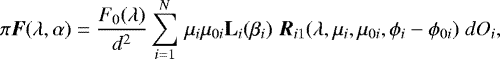
Fig. 1 Our model planet without clouds in F (top) and |Q| (bottom), using MODIS data of the following days (from left to right): July 1, July 28, August 24, September 20, October 17,November 13, and December 10, 2011, at various sub-observer longitudes and the following phase angles α: 0°, 20.41°, 40.82°, 60.25°, 90.49°, 109.92°, and 135.25°. The images are not a temporal sequence, they only illustrate various appearances of the planet. The RGB colors were computed using weighted additive color mixing of the fluxes at λ = 443 nm (blue), 550 nm (green), and 670 nm (red), such that when these fluxes are equal, the resulting color is white. The grayscale of each pixel is computed from the sum of the fluxes at the three wavelengths. These images have 220 pixels along the light equator of the planet. |
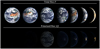 |
Fig. 2 Similar to Fig. 1, but with cloud properties and patterns from the MODIS data of the respective days. |
2.3 Computational costs
The computational costs of our numerical simulations depend on a large number of numerical parameter settings (Rossi et al. 2018; de Haan et al. 1987). For the results presented in this paper, and thus for the data files made publicly available, we chose the most accurate settings without considering the computational costs. In particular, with 100 pixels across the equator of the model planet, about 7850 pixels covered the planetary disk when we modeled the local variations in atmosphere and surface properties (see Sect. 3.1). For every local atmosphere-surface model, we computed the reflected Stokes vector (as coefficients of its expansion in a Fourier series, see Rossi et al. 2018) for up to 151 different local solar zenith angles θ0 and up to 151 different local viewing zenith angles θ. These Fourier-coefficient files were stored in a database for use in the computation of the disk-integrated Stokes vectors. For the latter, we used a temporal resolution for the rotation of the model planet of 15 min, covering 184 Earth days, thus 17 664 disk-integrations (with increasing α, the number of illuminated pixels on the planetary disk decreases, and the computational costs decrease in turn). With these settings, the computation of a disk-integrated Stokes vector across all phase angles takes about 18 h on a 2.7 GHz Intel Core i5 processor for a single wavelength.
3 Atmosphere – surface models
Here, we describe the local atmosphere and surface properties of the pixels on our model planet. We assign these properties using Earth-observation satellite data.
3.1 Model atmospheres
Our model planets have locally plane-parallel layered atmospheres that consist of gaseous molecules and (optionally) cloud particles. We assumed an Earth-like gas mixture in hydrostatic equilibrium (using an Earth-like gravitational acceleration g of 9.81 m s−2), with a mean molecular mass mg of 29 g mol−1. We only considered continuum wavelengths and thus ignored gaseous absorption. Our shortest wavelength of 350 nm is just outside the ultraviolet absorption band (the Huggins band) of ozone. For an Earth-like amount and vertical distribution of ozone, the broadband absorption between about 400 and 650 nm (the Chappuis band) decreases the total reflected flux at 550 nm wavelength, but it does not significantly affect the degree of polarization at this wavelength, because although in principle, absorption decreases the amount of multiple scattering of light, and thus usually increases the degree of polarization of the reflected light, most of the absorption by ozone takes place at high altitudes in the atmosphere,where the gas density and thus the amount of multiple scattering is small. The strength of absorption bands in reflected light signals depends on the (wavelength-dependent) absorption cross-section of the gas and also strongly depends on the amount and vertical distribution of the ozone molecules, and cloud particles. To avoid introducing too many Earth-specific parameters, we decided to ignore it (for spectra that include absorption by O3 in both the Huggins and the Chappuis bands, see Stam 2008).
The gas molecules are anisotropic Rayleigh scatterers with a wavelength-independent molecular depolarization factor δ of 0.03 (Hansen & Travis 1974) and a wavelength-dependent refractive index (Ciddor 1996). The surface pressure ps is 1.0 bar. Sample values of the atmospheric gaseous (scattering) optical thickness bg are 0.62 at λ = 350 nm and 0.043 at 670 nm. The atmospheric parameters and their values are given in Table 1.
We divided the atmosphere into three homogeneous layers. The gaseous scattering optical thickness of each layer was computed assuming an exponentially decaying pressure within each layer (for the radiative transfer algorithm, only the optical thickness of the layer is relevant, not the vertical distribution of the gas within the layer). If they were present, the cloud particles were in the middle layer. The cloud layer always had a vertical extent of 100 mb, and the pressurelevels of the three layers were adapted to accommodate different cloud top altitudes. Topographical variations were not considered, that is, the bottom of the atmosphere was at 1 bar everywhere, and the top was bounded by space. To limit the computational time and to avoid overcomplicating the models, our model atmospheres do not contain particles other than cloud particles, in other words, we ignored small, suspended, so-called aerosol particles such as dust and/or sea-salt particles, and/or smoke due to biomass burning. Most of these aerosol particles show significant horizontal variability while having relatively small optical thicknesses compared to clouds (for dust, see, e.g., Ginoux et al. 2001). The influence of various types and optical thicknesses of aerosol could be part of a subsequent study.
The spatial and temporal variability in the cloud cover is derived from observations by MODIS, the Moderate Resolution Imaging Spectroradiometer (for a detailed description of the MODIS data sets, including retrieval algorithms, see King et al. 2004; Parkinson & Greenstone 2000). We describe a cloud by the pressure of its top, pc, its optical thickness, bc, and the cloud particle size distribution and composition.
Each cloudy model pixel has a cloud fraction. This is zero for a cloud-free pixel. Even with as many as 100 pixels along the light equator of the model planet, the pixels are much larger than typical horizontal variations in clouds, and they are much larger than MODIS ground pixels. For a mixture of cloud-free and partly and fully cloudy MODIS ground pixels within a model pixel, we computed the locally reflected Stokes vector for a cloud-free and a cloudy model pixel, and took their weighted sum to compute the reflected Stokes vector for the pixel as a whole. In this way, we accounted for the cloud fraction as reported for all cloudy MODIS ground pixels. The mean cloud fraction of our model planet is about 66%.
The MODIS database provides a cloud top pressure for all of its pixels, and we computed pc of a cloudy model pixel by taking the average of the cloud top pressures of the MODIS pixels within our model pixel, weighted by their cloud fractions. To limit the number of different atmosphere-surface models, we divided pc for the model pixels into three categories: 500 mbar for 0 ≤ pc < 600 mbar, 700 mbar for 600 ≤ pc < 800 mbar, and 850 mbar for pc ≥ 800 mbar (see Table 1).
We computed bc for a cloudymodel pixel by taking the mean of the cloud optical thickness values of the MODIS ground pixels within the model pixel. In particular, we take the mean of the MODIS logarithmic daily mean data set (see Table 2). This data set provides the cloud optical thickness for a given MODIS pixel i as log bci, where bc i is the cloud optical thickness. When we computed the mean bc, we weighted logbci of each MODIS pixel with its cloudiness fraction. This logarithmic mean as a good approximation for the cloud optical thickness has been proposed by Hubanks et al. (2015) and Oreopoulos et al. (2007).
The wavelength at which a cloud optical thickness is provided in the MODIS data set depends on the surface: bc pertains to 645 nm above a dry surface, to 858 nm above an ocean, and to 1240 nm above snow or ice. We obtain bc at another wavelength by multiplying the value from the data set with the ratio of the cloud particle extinction cross-section at that other wavelength and at the given wavelength. The cloud optical thickness depends somewhat on the wavelength: for a cloud with bc = 10, composed of particles with reff = 12.5 μm and veff = 0.1, the cloud optical thickness, for example, ranges from 9.775 to 10.002, from 350 to 865 nm. The extinction cross-sections of the cloud particles were computed using a Mie-algorithm based on De Rooij & van der Stap (1984). To limit the number of different atmosphere-surface models, we divided bc for the model pixels into four categories: 0.0 when bc < 0.01, 5.0 when 0.01 ≤ bc < 7.5, 10.0 when 7.5 ≤ bc < 15.0, and 20 when bc > 15, at 645, 858, or 1240 nm, depending on the surface (see above).
The cloud particles were assumed to be homogeneous, liquid-water spheres, with a refractive index of n = 1.33 + 10−8i (Hale & Querry 1973). Their sizes are described by a two-parameter gamma distribution (Hansen & Travis 1974), with an effective particle radius reff and an effective variance veff. We used veff = 0.1 (Han et al. 1994; Nakajima & King 1990). The cloud particle effective radius was provided by the MODIS database, and we computed reff for a model pixel by taking the average of the effective radii of the MODIS pixels within our model pixel, weighted with the cloud fractions. We computed the single-scattering properties (i.e. single-scattering matrix, albedo, and extinction cross-section) of the cloud particles using a Mie algorithm based on De Rooij & van der Stap (1984).
To limit the number of different atmosphere-surface models, we divided reff for the model pixels into four categories (see Nakajima & King 1990): 10 μm for 0.0 ≤ reff ≤ 11.25 μm, 12.4 μm for 11.25 < reff ≤ 13.75 μm 15.0 μm for 13.75 < reff ≤ 16.25 μm, and 17.5 μm for reff > 16.25 μm.
Parameters of the model atmosphere.
3.2 Model surfaces
The surface of our model Earth was covered by four surface types: ocean, vegetation, soil, and snow or ice. Vegetation was subdivided into deciduous forest, grass, and steppe. Soil was subdivided into sand desert and shrubland. For the spatial and temporal variability in surface type we again used MODIS data. When the MODIS data showed various surface types within a model pixel,we assigned the most abundant surface type to the pixel. The different surface types and their reflection properties are described in more detail below.
3.2.1 Ocean
The ocean consisted of a Fresnel-reflecting and transmitting air-water interface with water below. The interface was rough due to wind-driven waves that were described by randomly oriented flat facets. The standard deviation of the wave-facet inclinations increased with the wind speed, widening the sun-glint pattern on the surface (Mishchenko & Travis 1997; Cox & Munk 1954). We includedscattering of light within the water body by describing it as a stack of horizontally homogeneous layers of pure seawater and by computing its reflection using an adding-doubling algorithm (de Haan et al. 1987). The sub-ocean surface was black.
The single scattering in pure seawater is described by anisotropic Rayleigh scattering (Hansen & Travis 1974) with a depolarization factor of 0.09 (Chowdhary et al. 2006; Morel 1974), combined with realistic absorption and scattering coefficients for pure seawater (Sogandares & Fry 1997; Pope & Fry 1997; Smith & Baker 1981). This results in a natural blue (for low chlorophyll concentrations) water body. The real part of the refractive index of the water was assumed to be 1.33 (Hale & Querry 1973) and wavelength independent, which does not significantly influence the ocean reflection. Furthermore, we took the reflection by wind-generated surface foam into account (see Koepke 1984) and corrected for the energy surplus across the rough air-water interface at grazing angles that was caused by neglecting wave shadowing (see also Zhai et al. 2010; Tsang et al. 1985).
To limit the number of different atmosphere-surface models, we divided the ocean surface wind speed v for the model pixels into two categories: 5 m s−1 for v < 6 m s−1, and 7 m s−1 for v ≥ 6 m s−1. This division is based on the global variation of mean wind speed measurements between January 1, 2011, and December 31, 2011, at an altitude of 10 meters (see Atlas et al. 2011)3. The parameters of the ocean properties are listed in Table 3. For a detailed description of our ocean reflection algorithm, see Trees & Stam (2019).
References of the parameter databases (upper part of the table) and of the surface models (lower part of the table) used for the Earth-like model planet.
Parameters of the ocean.
3.2.2 Vegetation
A vegetated surface on our model planet can be covered by deciduous forest, grass, or steppe. We used a combination of surface reflection models to describe the bidirectionally reflected total and linearly polarized fluxes. We also accounted for the reflection of incident linearly polarized light, as the diffuse skylight is usually linearly polarized. We ignored the reflection of incident circularly polarized light, however, as this signal is very weak (Rossi & Stam 2018). We also ignored the circular polarization of light that is reflected by vegetation. This light is expected to be slightly circularly polarized (Patty et al. 2019; Sparks et al. 2009), but to our knowledge, there is no numerical bidirectional reflection model for vegetation that includes circular polarization (the measurements by Patty et al. 2019 cover a range of incidence and reflection angles that is, as yet too limited to convert the data into a fully bidirectional reflection model).
To describe the bidirectionally reflected total flux, we used the numerical model developed by Roujean et al. (1992),
 (8)
(8)
where ρ is the bidirectional reflectance. The function f1 is the so-called geometric component of the reflection, which includes the influence of shadows (mutual shadows, such as one tree casting a shadow on another tree, are ignored), and f2 is the volume component, which includes the amount of local reflection (e.g. the density of leaves in a tree canopy) (for details, see Roujean et al. 1992). Functions f1 and f2 vanish at θ = θ0 = 0°. Using remote-sensing data, Roujean et al. (1992) derived parameters k0, k1, and k2 for various types of vegetation and two wavelength bands: 580 to 680 nm and 730 to 1100 nm.
To account for the spectral variability of the reflection within these bands, in particular the green bump and red-edge features, the k-parameters were scaled to the appropriate hemispherical albedo of the vegetation type considered. The hemispherical albedo of deciduous forest and grasslands was taken from the ECOSTRESS spectral library (Meerdink et al. 2019; Baldridge et al. 2009), and that of steppe from the Atmospheric Radiation Measurement research facility (ARM-facility 1998) (see Table 2).
To account for the reflected linearly polarized fluxes, we used a modified version of the numerical model developed by Maignan et al. (2009), following Schaepman-Strub et al. (2006), to obtain a bidirectional polarization distribution function (BPDF). This BPDF is a linear one-parameter-model, a simplification of the nonlinear, two-parameter model by Nadal & Breon (1999). To account for different types of vegetation, the BPDF uses the normalized difference vegetation index (NDVI) and a so-called α-parameter. A table with these parameters for several types of vegetation is provided in Maignan et al. (2009). With the NDVI parameter, the model of Maignan et al. (2009) accounts for the spectral variation in total flux, and with the α-parameter, a best fit with observations of the vegetation type considered is achieved (see Maignan et al. 2009, for a detailed description).
3.2.3 Arid regions
We used two types of arid regions: sandy deserts, and shrublands. For these surface types, we assumed the same reflection functions, but differentspectral albedos. We approximated the slightly polarized bidirectional reflection using the reflection matrix of an optically thick (i.e. bext = 100) layer of irregularly shaped mineral particles. This matrix was computed using our adding-doubling algorithm. For the single-scattering matrix of the mineral particles, we used that of the olivine S particles (Muñoz et al. 2012; Moreno et al. 2006), while we scaled the single-scattering albedo of the mineral particles to fit the hemispherical albedo of pale soil for the sandy desert, and dark brown entisol for the shrubland. The spectral albedos and databases we used are provided in Table 2.
3.2.4 Ice or snow cover
We described fields of snow and ice on land and inland waters as Lambertian reflectors. Their reflection is thus isotropic and unpolarized.A flat, smooth ice sheet free of rocks, snow or other rough materials might also be approximated as a Fresnel reflector. However, given the physical dimensions of our model pixels, and thus their spatial extent on the surface, a Lambertian approximation appears to be fitting well (Coakley 2003). To account for temporal changes in snow-covered land and inland water, we applied the daily global snow cover mask of MODIS on the yearly surface cover type data set. We did not account for sea ice. The names of the spectral albedo and surface type databases are provided in Table 2.
4 Results
4.1 RGB-images
Figures 1 and 2 show RGB images of our model Earth without and with clouds at various orientations and phase angles. These figures illustrate the variation in RGB colors of the total and polarized fluxes F and |Q| across the model planet. The model parameters are as described in Sect. 3. The RGB images clearly show that the disk-integrated fluxes are expected to vary spectrally and temporally as the planet rotates and orbits its star. A particularly striking feature on the cloud-free disks is the glint, that is, the sunlight that is reflected by the ocean, the contribution of which to the signal of the disk increases with increasing phase angle α. The glint can also be seen on the cloudy disks, but it is more diffuse, as clouds hide the ocean and its reflection from view. The reddening of the glint in F and |Q| with increasing α has been described by Trees & Stam (2019). These authors also argued that the reddening in |Q| is indicative of the presence of a cloud-free or cloudy ocean, while F also reddens when the planet has no ocean, but only clouds. The slight increase in |Q| of the cloudy model planet at α = 40° is due to the primary rainbow, that is, light that has been reflected inside the cloud droplets once (see, e.g., Karalidi et al. 2012b; Stam 2008; Bailey 2007).
4.2 Phase curves
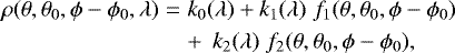
Figure 3 shows F, Q, U, V, and the degree of polarization P of light reflected by the rotating cloud-free model planet as functions of α, and for λ ranging from 350 to 865 nm. The simulations start at α = 0° on July 1, 12:00 GMT, 2011 (the geographic longitude centered at the illuminated and visible disk is 0°, like in Figs. 1–2), and stop at α = 180° on December 31, 11:45 GMT, 2011. The figure also includes curves for a cloud-free model planet whose surface is completely covered by ocean (the “ocean planet” phase curves of Fig. 1 of Trees & Stam 2019) with a surface wind speed v of 7 m s−1, instead of by a mixture of oceans and continents. Figure 4 is similar to Fig. 3, but has clouds. In Figs. 3 and 4, the thin lines were computed with a temporal resolution of 15 min, while the thicker, smoother lines are the averages over 24 h (α increases by about 1° in this period).
The two figures show that |U| is about a factor 100 smaller than |Q| across most of the phase angle range because our reference plane coincides with the light equator of the planet, and therefore any polarized flux |U| is due to secondary and higher-order scattered light, which has a low degree of polarization when integrated across the disk, even in the presence of horizontal inhomogeneities. The polarized flux |U| is highest at the shortest wavelengths because because there, the atmospheric gaseous optical thickness is highest there and thus more multiple scattering takes place. This is especially apparent for the cloudy model planet, where multiple scattering in the gaseous atmosphere above the clouds produces much more |U| at 350 nm than at 443 nm, where the gas optical thickness above the clouds is far lower.
The circularly polarized flux |V | is a factor ofabout 104 lower than Q. This flux only arises for light that has been scattered at least twice, including at least once by the cloud particles, as Rayleigh scattering alone does not produce circular polarized fluxes (see Rossi & Stam 2018, and references therein). When a model planet is mirror-symmetric with respect to the planetary scattering plane, the circularly polarized flux of the hemisphere above the scattering plane (the northern hemisphere) will be equal to that of the hemisphere below the scattering plane (the southern hemisphere), except for the sign: because of the mirror symmetry in the scattering geometries, V of the northern hemisphere equals − V of the southern hemisphere (see García Muñoz 2015, for comparable phase curves of V∕I as computed for the two hemispheres of the Earth, except with a black surface to model the ocean, while our ocean is modelled as a rough, Fresnel reflecting surface with scattering in the water body below). Integrated over the planetary disk, V of a mirror-symmetric planet will thus equal zero. For a horizontally inhomogeneous planet, such as our model planets, the disk-integrated |V | is usually not zero, but it is still very small, and it decreases with λ as the atmosphere’s Rayleigh scattering optical thickness decreases with the wavelength. The circular polarization signature of light scattered by chiral molecules, such as those found e.g. in the cells making up Earth-like vegetation, on the northern hemisphere will have the same sign as that on the southern hemisphere, and will thus not be cancelled when integrated across the planetary disk, even though the total signal will still be small because the fraction of circularly polarized flux that is reflected by chiral molecules is very small (see Patty et al. 2019).
Figures 3 and 4 show that except at α > 120°, the average (24 h) total and polarized fluxes decrease with increasing λ below 670 nm. The reason is that the Rayleigh scattering optical thickness in the atmosphere decreases with λ (our model atmospheres contain no ozone, otherwise the fluxes at 350 nm would have been much lower than shown here), and because the dark ocean suppresses the terrestrial average surface albedo. The total flux F at 865 nm is an exception: it is higher than at 670 nm (for α < 120°). The reason is that at 865 nm, the albedo of vegetation is higher than at 670 nm. The increase in this albedo with increasing λ above about 670 nm is usually referred to as the red edge (Montañés-Rodríguez et al. 2006; Seager et al. 2005). Because of the low-polarization signature of the vegetation, |Q| at 865 nm is lower than at 670 nm.
For α > 120°, the average (24 h) cloud-free model planet changes color from blue through white to red because of the presence of the Fresnel-reflecting ocean (see Fig. 1 in Trees & Stam 2019). The contribution of the ocean glint (which itself is spectrally neutral) increases with increasing λ as the Rayleigh scattering optical thickness in the atmosphere decreases. Trees & Stam (2019) showed that in F, this color change may also result from Rayleigh-scattering gas above the clouds, that is, also in the absence of an ocean. The diurnal average of P changes color at α ~ 144° and the diurnal average of Q changes color at α ~ 138°. Trees & Stam (2019) postulated that the color change of P from blue through white to red with increasing α identifies a partly cloudy exo-ocean, while the color change in Q uniquely identifies an exo-ocean, independent of the surface pressure or cloud fraction.
Compared with the results in Trees & Stam (2019), where all model planets were ocean planets, Figs. 3 and 4 show that when the model planet has oceans and continents, P and Q still change color, and their color change is thus still indicative of the presence of an ocean. On Earth, 71% of the surface is covered by ocean, and in the equatorial regions where the glint occurs, the coverage is even higher.
The average (24 h) F, Q, and P phase curves of the cloudy planet (Fig. 4) show the familiar features that are due to the scattering of light by the cloud particles, in particular the primary rainbow near α = 40° that is due to light that has been reflected once within the spherical liquid-water droplets (Karalidi et al. 2011; Stam 2008; Bailey 2007), an enhancement that was also identified in Fig. 2. Fluxes U and V also appear to have a feature at the primary rainbow angle, although not very obvious. At phase angles below 5°, the curves show a small enhancement that is due to the glory formed by light that is back-scattered by the spherical cloud droplets (see, e.g., Hansen & Travis 1974; Bryant & Jarmie 1974). At such small phase angles, an exoplanet would be extremely close to its star.
The close-ups of the diurnal variations (the 15 min curves) in Fig. 3 show patterns that repeat about every 1° in α and are caused by continents and oceans that rotate in and out of view. In Fig. 4 the clouds add variation to the modulation through the surface features and thus suppress the repeated patterns. The temporal variation in F, Q, and P increases with increasing α because with decreasing illuminated area on the planetary disk, local variations in surface and cloud coverage contribute more prominently to the reflected signal, as also described by Stam (2008), for example. With increasing α, the contribution of the ocean glint to F and Q also increases (cf. Fig. 2). At short wavelengths, the peak-to-peak variability in F and Q of the cloud-free planet (Fig. 3) is small because the Rayleigh scattering optical thickness of the atmosphere is high and suppresses the surface signals. With increasing λ, the Rayleigh scattering decreases and the peak-to-peak variations due to surface albedo variations are increasingly visible.
In the presence of clouds (Fig. 4), Q and the very low fluxes U and V show the strongest peak-to-peak variability at the shortest wavelength (350 nm). The temporal variations in U and V appear to be inversely correlated at small α and correlated at larger α, which can probably be explained by the fact that both U and V are due to multiple scattered light. The precise relation requires further investigations, however. This strong variability is correlated with the variability of the clouds: without clouds, the polarized fluxes are due to incident sunlight that is scattered upward by the atmospheric gases. Clouds strongly increase the total flux that is reflected by a pixel, and while P of the flux reflected by the cloud is usually low, part of this reflected light is scattered in the gas above the cloud before it escapes into space. Because this last scattering is in the gas, it significantly adds in particular to the planetary linearly polarized flux Q. With increasing λ, the amount of light that is scattered in the gas above the cloud decreases, and with this, the contribution to the polarized fluxes and the sensitivity to the cloud variability decrease.
Robinson et al. (2011) and Fujii et al. (2011) studied the diurnal variability in Earth’s reflected total flux F and compared results from their numerical models to reflected total-flux observations of the Earth taken by the EPOXI mission (on three separate days in 2008, at α = 57.7°, 75.1°, and 76.6°, respectively, although Fujii et al. 2011 did not use the 75.1° data because the moon was partially in view), while Jiang et al. (2018) analyzed reflected total-flux data of the DSCOVR mission (taken only at α = 0°). García Muñoz (2015) used his radiative transfer code to simulate 2005 MESSENGER data (reflected total fluxes) between α =98° to 107°. While quantitative comparisons between our computed reflected total fluxes and the measured data and computed fluxes presented in these papers is difficult because of differences in cloud coverage and orientation of the model planet (when limited phase angles are covered in the observations), and because different definitions were used, for instance (e.g., fluxes are shown as normalized to a 24 h time average). We can, however, perform a qualitative comparison (only for the total fluxes because polarized fluxes of the Earth as a whole, have not been measured from space).
In general, Robinson et al. (2011) and Fujii et al. (2011) reported a similar increase in the peak-to-peak variability of the reflected F data with increasing λ as we, and the wavelength dependence of F is similar (across the phase-angle range of the EPOXI data); the Earth is darkest around 650 nm (Fujii et al. 2011)or 670 nm (our simulations). Jiang et al. (2018) showed a stronger peak-to-peak variability in F at 780 nm than at 380 nm at the 0° phase angle of the DSCOVR data (the spectral solar flux was included in the reflected flux data in their paper). Our diurnal curves as shown in Fig. 4 (diurnal curves near full-phase) agree (qualitatively) well with DSCOVR observations, with strong enhancements in F when large convective clouds near the maritime continents and the Atlantic side of the American continent are in view (see Jiang et al. 2018). The reflected MESSENGER fluxes reported by García Muñoz (2015) show the same dependence of F on λ, but a less obvious stronger peak-to-peak variability with increasing wavelength. This might be explained by the smaller wavelength range that is covered by the MESSENGER data, as only 480, 560„ and 630 nm are shown by García Muñoz (2015).
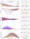 |
Fig. 3 Numerical results for the cloud-free model Earth. Left: total flux F, linearly polarized fluxes Q and U, circularly polarized flux V, and degree of polarization P as functions of α at λ = 350 nm (pink lines), 443 nm (blue), 550 nm (green), 670 nm (red), and 865 nm (brown). The temporal resolution of the thin lines is 15 min. The thick solid lines are the diurnal (24 h) averages. At α = 0°, the time is July 1, 12:00 GMT, 2011. At α = 180°, the time is December 31, 11:45 GMT, 2011. The thick dashed lines are the diurnal averages of a cloud-free “ocean planet” (cf. Fig. 1 of Trees & Stam 2019), thus of a planet without clouds and continents. Right: close-ups of the 15-min time-resolution phase curves for two phase-angle regions as functions of the longitude in the middle of the longitude range that is visible to the observer. The background of each close-up shows the corresponding geographic map of Earth. Note the different vertical scales. |
4.3 Color changes
In Fig. 5 we show the colors of our cloudy model planet (with an average cloud fraction of about 66%) in F, Q, and P as functions of the geographic longitude in the middle of the longitude range on the illuminated and visible part of the planetary disk, and phase angle α (these are functions of time themselves, i.e., with increasing longitude, α also slightly increases), computed using the curves at 443, 550, and 670 nm in Fig. 4. With increasing α, the effect of the local patterns on the planet starts to appear, as the illuminated and visible part of the planetary disk decreases.
Figure 5 shows how the planet changes color in F from blue through white to red with increasing α. The planet appears white when the phase curves of F at λ= 443, 550 and 670 nm intersect (cf. Fig. 4), which is near α =120°, in Fig. 5. The faint white vertical stripe near α = 40° is due to the primary rainbow. This rainbow feature is much stronger in Q and P. Flux F shows a few whitish, horizontal streaks that are related to the presence of continents around those longitudes, in particular, Africa (around 30°) and the Americas (around 300°). At smaller phase angles, the brown and green color of the arid and vegetated regions comprising the largest regions of the continents (see Fig. 2) compensate for the blueness of the atmosphere, while at the larger phase angles, the continents limit the reflection by the ocean that tends to color a planet red at these phase angles (Trees & Stam 2019).
The color changes in polarized flux Q and degree of polarization P appear to be related to the visibility of an ocean surface depending on which part of the planet is visible to the observer. Trees & Stam (2019) have derived that for ocean planets, that is, planets without continents, the color change phase angle for F decreases with increasing cloud coverage fraction fc, while it increases with increasing fc for Q and P. In Fig. 5, F changes color in a 5–10° wide phase-angle range around 120°, which on an ocean planet would be indicative for fc ranging from 0.25 to 0.75 (Trees & Stam 2019). However, on these model planets, the continental surface coverage and the surface albedo of the continents also affects the color of F. According to Trees & Stam (2019), for Q and P of ocean planets, the phase angle where the color changes increases with increasing fc, and Fig. 5 shows that adding continents (partly) below the clouds appears to have a similar effect: for longitudes with more continental coverage, the color-changing phase angle is larger than for longitudes with less continental coverage (assuming that the clouds are more or less evenly distributed across the planet).
A tentative color crossing in polarized Earth-shine observations has recently been presented by Sterzik et al. (2019). These measurements were obtained with ESO’s Very Large Telescope (VLT). Given the telescope location in Chile, either the Pacific Ocean or South America and the Atlantic Ocean would have been oriented toward the Moon, depending on the time of the observations. The Pacific Ocean observations cover the widest phase-angle range (from about 50° to 135°) and show a tentative color crossing near 135°. This phase angle is similar to what is shown in Fig. 5. The Atlantic Ocean observations cover phase angles from about 65° to 116°, which is not far enough to actually show a color-crossing phase angle, but extrapolation by eye suggests a crossing phase-angle between 125° and 130°, which would be smaller than shown in Fig. 5. This might be due to a different orientation of the Earth than used in our simulations or to different cloud properties. The precise relation between the color-changing phase angle, the surface coverage, and the (variable) cloud coverage and its applicability in characterizing the distribution of continents and ocean on exoplanets will be subject of a later study.
 |
Fig. 5 RGB colors of F (top), Q (middle), and P (bottom) of the cloudy model planet as functions of phase angle α and thelongitude in the middle of the longitude range that is visible to the observer (0° longitude corresponds with the Greenwich meridian). These color plots were constructed from the F, Q, and P phase curves at 443, 550 and 670 nm as presented in Fig. 4. The horizontal black lines indicate the respective longitudes on the geographical map on the right. |
5 Summary and discussion
We have presented numerically computed total and polarized fluxes of starlight that is reflected by an Earth-like model planet as functions of time, the planetary phase angle, and for five different wavelengths in the continuum: 350, 443, 550, 670, and 865 nm. These fluxesand the derived degree of polarization can play a crucial role as test data to help the design and development of astronomical instrumentation and observational strategies for the direct detection of small Earth-like exoplanets, especially because such data (across time, phase angles, and wavelength) are unavailable from Earth-observation missions.
Estimates show that with a dedicated technology maturation path, strategic exo-Earth characterization missions might be possible around 2030-2035 (Crill & Siegler 2017). This estimate is based on an extensive study of current technology areas that must be advanced to image exo-Earths, albeit including only brightness (total flux) measurement techniques. Similarly, Feng et al. (2018) estimated the science return of space observatories such as HabEx and LUVOIR for different instrument designs with an inverse-modeling framework. They also considered only total fluxes.
With our results, the advantages of including spectropolarimetry can be studied on the instrument and mission level. In particular, our results can be used to investigate the effect of the polarimetric accuracy that can be achieved by different polarimetrictechniques in an instrument and by different telescope designs, especially the effects of various advanced adaptive optics techniques, and different types of coronagraphs to reduce the background stellar flux and to optimize the inner working angle. By integrating our results over time, effects of observational integration times can be investigated.
Specific phase-angle-dependent features that would be worth detecting appear to be the primary rainbow as a tool for detecting liquid water clouds (as earlier identified, e.g., by Karalidi et al. 2012b; Bailey 2007), which is a stronger signal in Q and P than in F, the color-crossing phase angle in Q or P as a tool fordetecting liquid surfaces (for details, see Trees & Stam 2019), and the regular variations due to the daily rotation of the planet and the variability on those variations due to the changing cloud cover. When the orientation of the planetary light equator with respect to the instrumental optical plane is not known, because the orientation of the planetary orbit is not known, the distribution of linearly polarized flux over Q and U is generally different than in our results. The very low values of |U| as compared to |Q| when the instrumental reference plane is parallel to the light equator, even for a horizontally inhomogeneous planet like the Earth, could be used to determine the orientation of the light equator, and with this, of the orbit.
Because the diurnal variability of the signals appears to be little dependent on the wavelength, except for |Q| at short wavelengths, broadband observations would help increase the signal-to-noise ratio (S/N) of observations (see Bailey 2007, for a similar discussion on the observability of the rainbow feature). At short wavelengths (λ = 350 nm in our results), the variability of |Q| strongly depends on the cloud properties and very little on the surface properties. Measuring in a short and a long wavelength band would therefore allow for uncoupling cloud and surface reflection. The color-crossing α for liquid surface detection is at a relatively large phase angle, that is, near 145° for an Earth-like cloud coverage fraction (the larger the coverage fraction, the larger the color-crossing phase angle, see Trees & Stam 2019), and F, |Q| and P are relatively small at these phase angles. In addition, the color of the planet should be determined, and observations through more than one spectral band should therefore be performed. However, the color-crossing can be detected across a range of phase angles of 10°–20° wide, which would allow for long integration times, see Fig. 5.
Our polarized flux results are valuable test data not only for spectropolarimeters, instruments designed to measure polarization, but also for spectrometers, instruments that might not have been designed to measure polarization, but that are often polarization sensitive due to the use of optical elements such as mirrors and gratings. Without a proper validation of the design of a spectrometer for incident light that is polarized, such as starlight that is reflected by an exoplanet, measurement errors arise that are hard to account for. When test data are used in combination with instrument simulators, the errors for a given design can be estimated and the design can be adapted to minimize them.
Because the physical parameters of our model Earth are known, our computed fluxes and the degree of polarization across time, phase angle, and wavelength can also be used to develop and/or test data analysis algorithms to be used on (future) measurements of light reflected by exoplanets, such as autocorrelation methods of the Fourier analysis to derive the planetary rotational period and/or the presence of continents (see Visser & van de Bult 2015; Oakley & Cash 2009; Pallé et al. 2008). To simulate actual measurements, our total and polarized fluxes would have to be scaled tothose of the target exoplanet and its star, according to Eq. (7), noise sources (photon noise and background stellar light) and instrumental effects (e.g. derived from a preliminary design) could be added, by scaling the computed fluxes and/or integrating across instrument response functions, effects of different integration times and/or spectral resolutions can be studied. Our computed total and polarized fluxes could also be combined with total and polarized fluxes of light of the parent star that is scattered by exo-zodiacal dust (see, e.g., Renard et al. 1995) to investigate the effect of such local background sources on the detectability of the planetary signals.
For our model planet, we used Earth-observation data covering the period from January 1, 2011, to December 31, 2011, to describe the surface coverage and local albedos, the cloud coverage fraction, optical thickness, top pressure, and the effective radius of the cloud particles. The surface types that we took into account are oceans (with waves), vegetation (deciduous forest, grass, and steppe), arid regions (desert and shrublands), and ice or snow. The reflection by the ocean and arid regions fully includes linear (and circular) polarization, while that by the vegetation only includes linear polarization. Ice and snow are described by a Lambertian, that is, isotropic and unpolarized.
For the numerical results presented here, we did not include scattering and absorption by aerosol particles (small, suspended particles in the atmosphere): although numerically they are straightforward to include, their variations in space and time would require the addition of many atmosphere-surface models and hence severely increase the computing times. Zugger et al. (2011, 2010) investigated the effects of spherical maritime (sea-salt) aerosol particles (which are likely nonspherical, see Mishchenko et al. 2000) on the polarized reflection of ocean planets and concluded that depending on the visibility, these aerosols could significantly depolarize the reflected fluxes, although a comparison between the Earth-shine observations and model computations without aerosol presented by Sterzik et al. (2019) strongly suggests that aerosols in general have a minor effect on the polarized appearance of Earth, especially when compared to the effects of clouds (which Zugger et al. 2011, 2010 did not combine with the maritime aerosol). Our model atmospheres do not include (nonspherical) ice cloud particles either; all cloud particles are liquid water droplets. Scattering by nonspherical ice cloud particles was included by Karalidi et al. (2012b), who used both liquid water clouds and ice clouds in their model atmospheres. The ice- and liquid-cloud optical thicknesses were derived from MODIS data. They adopted imperfectly shaped hexagonal ice-cloud particles (Hess 1998), and concluded among others, that the presence of ice clouds does not limit the visibility of the rainbow (which is due to spherical particles alone) in the polarization. Emde et al. (2017) used both types of cloud particles and relatively high ice-cloud optical thicknesses in their analysis of the polarized Earth-shine data published by Sterzik et al. (2012).
Our numerical computations do not include the absorption of light by atmospheric gases either, such as water and oxygen. This absorption can be included and will lead to features with high spectral resolution polarization across the absorption bands (see, e.g., Fauchez et al. 2017; Stam 2008), so that our fluxes should be considered to be representative of the continuum. Absorption by ozone is also neglected. This would be important to be included when wavelengths below 350 nm are of interest. The wavelength of 550 nm falls within a broad diffuse ozone absorption band (the Chappuis band) that would lower the reflected total and polarized fluxes, especially in the presence of clouds, but it would hardly change the degree of polarization (see, e.g., Stam 2008). We also ignored rotational Raman scattering, which is an inelastic scattering process by gaseous molecules, which would leave imprints of the stellar Fraunhofer lines in the total and polarized fluxes and in the degree of polarization as functions of the wavelength. In Earth observations, this phenomenon is usually referred to as the Ring effect after one of the discoverers (Grainger & Ring 1962). Numerical simulations of rotational Raman scattering in atmospheres of gas giants (in total fluxes only) has been presented by Oklopčić et al. (2016). Rotational Raman scattering could be added to our numerical algorithm, but would require significant amounts of computing time.
Some improvements of our descriptions of the surface reflection are the reflection by the surface below shallow waters, altitude variations on the surface, such as mountains, regions of the ocean covered by sea ice, and seasonal variations in the surface reflection. Regarding the latter, in particular, seasonal albedo changes due to the migration of sea ice over the ocean, for instance, changes in the colors of vegetation, in the bloom of algae, etc. could be implemented. Polarization measurements of locally scattered and/or reflected light, for example, by instruments on board satellites in low Earth orbits, would be very useful for the extension and/or improvement of the currently missing or insufficient numerical descriptions of scattered or reflected light, as described above.
While validation of computed disk-integrated total and/or polarized fluxes reflected by a model Earth can be made somewhat using (polarized) Earth-shine measurements (see Sterzik et al. 2012), this method has several limitations, in particular, the unknown influence of the reflection of Earth-light by the lunar surface. While we can in principle measure how the surface (at different locations on the Moon) reflects incident (unpolarized) sunlight for various local solar zenith angles and various local viewing angles, we do not know how the surface reflects polarized light, especially not as a function of wavelength and covering a range of illumination and viewing geometries. Sterzik et al. (2019) presented a method to correct their polarized Earth-shine measurements for the lunar depolarization effect, but the uncertainty in this method appears to be too large to validate parameter choices for the model planets. The ideal validation data would be spectropolarimetric measurements of the Earth taken from a distance. A compact instrument that would provide such data is the LOUPE (Hoeijmakers et al. 2016; Karalidi et al. 2012a), which aims to measure the total flux and the degree and direction of linear polarization from about 400 to 800 nm as the payload of a lunar lander or a geostationary satellite, for example (the latter would, however, not allow monitoring signal variations because the planet rotates daily). The spectropolarimeter LSDpol also aims to measure circular polarization across a similar spectral range 350–900 nm (Snik et al. 2019).
The computed total and polarized fluxes are available through the database researchdata.4tu.nl. They are archived under “Colors of an Earth-like exoplanet” with DOI 10.4121/uuid:caa03e1a-0f6a-43e5-b67a-fa6f21829b8a
Acknowledgements
The MODIS Land Cover Type Data set (2011) is maintained by the NASA EOSDIS Land Processes Distributed Active Archive Center (LP DAAC) at the USGS/Earth Resources Observation and Science (EROS) Center. The Aqua/MODIS and Terra/MODIS Cloud Top Pressure, Cloud Particle Effective Radius, Cloud Optical Thickness and Cloud Fraction Daily L3 Global 1 Deg. CMG datasets were acquired from the Level-1 and Atmosphere Archive & Distribution System (LAADS) Distributed Active Archive Center (DAAC), from the Goddard Space Flight Center in Greenbelt, Maryland, USA (https://ladsweb.nascom.nasa.gov/). The CCMP Version-2.0 vector wind analyses are produced by Remote Sensing Systems, with data available at www.remss.com. We acknowledge the use of the SCIAMACHY surface LER database provided by the Royal Netherlands Meteorological Institute (KNMI). L.R. acknowledges funding through the Planetary and Exoplanetary Science (PEPSci) Programme of the Netherlands Organisation for Scientific Research (NWO).
References
- Aizawa, M., Kawahara, H., & Fan, S. 2020, ApJ, 896, 22 [CrossRef] [Google Scholar]
- ARM-facility 1998, Surface Spectral Albedo (SURFSPECALB1MLAWER). 2011/06/20 to 2011/06/20, Southern Great Plains (SGP) Central Facility, Lamont, OK (C1). Compiled by K. Gaustad and L. Riihimaki. Atmospheric Radiation Measurement (ARM) Data Center, http://dx.doi.org/10.5439/1095394 [Google Scholar]
- Atlas, R., Hoffman, R. N., Ardizzone, J., et al. 2011, Bull. Am. Meteorol. Soc., 92, 157 [CrossRef] [Google Scholar]
- Bailey, J. 2007, Astrobiology, 7, 320 [NASA ADS] [CrossRef] [PubMed] [Google Scholar]
- Baldridge, A. M., Hook, S. J., Grove, C. I., & Rivera, G. 2009, Remote Sens. Environ., 113, 711 [CrossRef] [Google Scholar]
- Bazzon, A., Schmid, H. M., & Gisler, D. 2013, A&A, 556, A117 [NASA ADS] [CrossRef] [EDP Sciences] [Google Scholar]
- Bean, J. L., Miller-Ricci Kempton, E., & Homeier, D. 2010, Nature, 468, 669 [NASA ADS] [CrossRef] [PubMed] [Google Scholar]
- Berdyugina, S. V., & Kuhn, J. R. 2019, AJ, 158, 246 [CrossRef] [Google Scholar]
- Berdyugina, S. V., Berdyugin, A. V., Fluri, D. M., & Piirola, V. 2011, ApJ, 728, L6 [NASA ADS] [CrossRef] [Google Scholar]
- Bétrémieux, Y., & Kaltenegger, L. 2014, ApJ, 791, 7 [NASA ADS] [CrossRef] [Google Scholar]
- Bouret, J.-C., Neiner, C., Gómez de Castro, A. I., et al. 2018, SPIE Conf. Ser., 10699, 106993B [Google Scholar]
- Bryant, H. C., & Jarmie, N. 1974, Sci. Am., 231, 60 [CrossRef] [Google Scholar]
- Chou, F., Johnson, M., & Landau, E. 2017, NASA Releases Kepler Survey Catalog with Hundreds of New Planet Candidates, https://www.nasa.gov/ [Google Scholar]
- Chowdhary, J., Cairns, B., & Travis, L. D. 2006, Appl. Opt., 45, 5542 [NASA ADS] [CrossRef] [Google Scholar]
- Ciddor, P. E. 1996, Appl. Opt., 35, 1566 [NASA ADS] [CrossRef] [PubMed] [Google Scholar]
- Coakley, J. 2003, Reflectance and Albedo Surface (New York: Academic Press), 1914 [Google Scholar]
- Cotton, D. V., Marshall, J. P., Bailey, J., et al. 2017, MNRAS, 467, 873 [NASA ADS] [Google Scholar]
- Cox, C., & Munk, W. 1954, J. Opt. Soc. Am. 1917–1983, 44, 838 [NASA ADS] [CrossRef] [Google Scholar]
- Crill, B. P., & Siegler, N. 2017, SPIE Conf. Ser., 10398, 103980H [Google Scholar]
- de Haan, J. F., Bosma, P. B., & Hovenier, J. W. 1987, A&A, 183, 371 [Google Scholar]
- De Rooij, W. A., & van der Stap, C. C. A. H. 1984, A&A, 131, 237 [NASA ADS] [Google Scholar]
- Deschamps, P. Y., Breon, F. M., Leroy, M., et al. 1994, IEEE Trans. Geosci. Remote Sens., 32, 598 [NASA ADS] [CrossRef] [Google Scholar]
- Dubovik, O., Li, Z., Mishchenko, M. I., et al. 2019, J. Quant. Spectr. Rad. Transf., 224, 474 [CrossRef] [Google Scholar]
- Emde, C., Buras-Schnell, R., Sterzik, M., & Bagnulo, S. 2017, A&A, 605, A2 [NASA ADS] [CrossRef] [EDP Sciences] [Google Scholar]
- Fan, S., Li, C., Li, J.-Z., et al. 2019, ApJ, 882, L1 [NASA ADS] [CrossRef] [Google Scholar]
- Fauchez, T., Rossi, L., & Stam, D. M. 2017, ApJ, 842, 41 [NASA ADS] [CrossRef] [Google Scholar]
- Feng, Y. K., Robinson, T. D., Fortney, J. J., et al. 2018, AJ, 155, 200 [NASA ADS] [CrossRef] [Google Scholar]
- Ford, E. B., Seager, S., & Turner, E. L. 2001, Nature, 412, 885 [NASA ADS] [CrossRef] [PubMed] [Google Scholar]
- Fougnie, B., Bracco, G., Lafrance, B., et al. 2007, Appl. Opt., 46, 5435 [CrossRef] [Google Scholar]
- Friedl, M., & Sulla-Menashe, D. 2019, MCD12Q1 MODIS/Terra+Aqua Land Cover Type Yearly L3 Global 500m GEO Grid V006. NASA EOSDIS Land Processes DAAC, https://doi.org/10.5067/MODIS/MCD12C1.006 [Google Scholar]
- Fujii, Y., Kawahara, H., Suto, Y., et al. 2011, ApJ, 738, 184 [CrossRef] [Google Scholar]
- García Muñoz, A. 2015, Int. J. Astrobiol., 14, 379 [CrossRef] [Google Scholar]
- García Muñoz, A., Zapatero Osorio, M. R., Barrena, R., et al. 2012, ApJ, 755, 103 [NASA ADS] [CrossRef] [Google Scholar]
- Gilbert, E. A., Barclay, T., Schlieder, J. E., et al. 2020, AJ, submitted, [arXiv:2001.00952] [Google Scholar]
- Ginoux, P., Chin, M., Tegen, I., et al. 2001, J. Geophys. Res., 106, 255 [CrossRef] [Google Scholar]
- Ginski, C., Benisty, M., van Holstein, R. G., et al. 2018, A&A, 616, A79 [NASA ADS] [CrossRef] [EDP Sciences] [Google Scholar]
- Grainger, J. F., & Ring, J. 1962, Nature, 193, 762 [NASA ADS] [CrossRef] [Google Scholar]
- Hale, G. M., & Querry, M. R. 1973, Appl. Opt., 12, 555 [NASA ADS] [CrossRef] [PubMed] [Google Scholar]
- Hall, D. K., & Riggs, G. A. 2016, MODIS/Aqua Snow Cover Daily L3 Global 500m SIN Grid, Version 6. MYD10C1. Boulder Colorado USA. NASA National Snow and Ice Data Center Distributed Active Archive Center, https://doi.org/10.5067/MODIS/MOD10A1.006 [Google Scholar]
- Han, Q., Rossow, W. B., & Lacis, A. A. 1994, J. Clim., 7, 465 [NASA ADS] [CrossRef] [Google Scholar]
- Hansen, J. E., & Travis, L. D. 1974, Space Sci. Rev., 16, 527 [NASA ADS] [CrossRef] [Google Scholar]
- Hess, M. 1998, J. Quant. Spectr. Rad. Transf., 60, 301 [NASA ADS] [CrossRef] [Google Scholar]
- Hoeijmakers, H. J., Arts, M. L. J., Snik, F., et al. 2016, Opt. Express, 24, 21435 [NASA ADS] [CrossRef] [Google Scholar]
- Hovenier, J. W., & van der Mee, C. V. M. 1983, A&A, 128, 1 [NASA ADS] [Google Scholar]
- Hovenier, J. W., Van Der Mee, C., & Domke, H. 2004, Astrophys. Space Sci. Lib., 318 [Google Scholar]
- Hubanks, P., Platnick, S., King, M., & Ridgway, B. 2015, ATBD reference number ATBD-MOD-30, NASA, 125 [Google Scholar]
- Jiang, J. H., Zhai, A. J., Herman, J., et al. 2018, AJ, 156, 26 [NASA ADS] [CrossRef] [Google Scholar]
- Kaltenegger, L., & Traub, W. A. 2009, ApJ, 698, 519 [NASA ADS] [CrossRef] [Google Scholar]
- Karalidi, T., Stam, D. M., & Hovenier, J. W. 2011, A&A, 530, A69 [NASA ADS] [CrossRef] [EDP Sciences] [Google Scholar]
- Karalidi, T., Stam, D. M., Snik, F., et al. 2012a, Planet. Space Sci., 74, 202 [NASA ADS] [CrossRef] [Google Scholar]
- Karalidi, T., Stam, D. M., & Hovenier, J. W. 2012b, A&A, 548, A90 [NASA ADS] [CrossRef] [EDP Sciences] [Google Scholar]
- Kasper, M., Beuzit, J.-L., Verinaud, C., et al. 2010, SPIE Conf. Ser., 7735, 77352E [Google Scholar]
- Kawahara, H., & Fujii, Y. 2011, ApJ, 739, L62 [CrossRef] [Google Scholar]
- Kawata, Y. 1978, Icarus, 33, 217 [NASA ADS] [CrossRef] [Google Scholar]
- Keller, C. U., Schmid, H. M., Venema, L. B., et al. 2010, SPIE Conf. Ser., 7735, 77356G [Google Scholar]
- Kemp, J. C., Henson, G. D., Steiner, C. T., Beardsley, I. S., & Powell, E. R. 1987, Nature, 328, 92 [CrossRef] [Google Scholar]
- Kiang, N. Y., Segura, A., Tinetti, G., et al. 2007a, Astrobiology, 7, 252 [NASA ADS] [CrossRef] [Google Scholar]
- Kiang, N. Y., Siefert, J., Govindjee, & Blankenship, R. E. 2007b, Astrobiology, 7, 222 [CrossRef] [Google Scholar]
- King, M. D., Closs, J., Spangler, S., et al. 2004, EOS Data Products Handbook Volume 1, https://eospso.nasa.gov/sites/default/files/publications/data_products_1.pdf [Google Scholar]
- Koepke, P. 1984, Appl. Opt., 23, 1816 [NASA ADS] [CrossRef] [Google Scholar]
- Kostogryz, N. M., Yakobchuk, T. M., & Berdyugina, S. V. 2015, ApJ, 806, 97 [NASA ADS] [CrossRef] [Google Scholar]
- Maignan, F., Bréon, F.-M., Fédèle, E., & Bouvier, M. 2009, Remote Sens. Environ., 113, 2642 [CrossRef] [Google Scholar]
- Mayor, M., & Queloz, D. 1995, Nature, 378, 355 [Google Scholar]
- Meerdink, S. K., Hook, S. J., Roberts, D. A., & Abbott, E. A. 2019, Remote Sens. Environ., 230, 111196 [CrossRef] [Google Scholar]
- Miles-Páez, P. A., Pallé, E., & Zapatero Osorio, M. R. 2014, A&A, 562, L5 [NASA ADS] [CrossRef] [EDP Sciences] [Google Scholar]
- Millar-Blanchaer, M. A., Girard, J. H., Karalidi, T., et al. 2020, ApJ, 894, 42 [CrossRef] [Google Scholar]
- Mishchenko, M. I., & Travis, L. D. 1997, J. Geophys. Res., 102, 16989 [NASA ADS] [CrossRef] [Google Scholar]
- Mishchenko, M. I., Hovenier, J. W., & Travis, L. D. 2000, Light scattering by nonspherical particles : theory, measurements, and applications (San Diego: Academic Press) [Google Scholar]
- Misra, A., Meadows, V., & Crisp, D. 2014, ApJ, 792, 61 [CrossRef] [Google Scholar]
- Montañés-Rodríguez, P., Pallé, E., Goode, P. R., & Martín-Torres, F. J. 2006, ApJ, 651, 544 [NASA ADS] [CrossRef] [Google Scholar]
- Morel, A. 1974, Opt. Aspects Oceanogr., 1, 1 [Google Scholar]
- Moreno, F., Vilaplana, R., Muñoz, O., Molina, A., & Guirado, D. 2006, J. Quant. Spectr. Rad. Transf., 100, 277 [NASA ADS] [CrossRef] [Google Scholar]
- Muñoz, O., Moreno, R., Guirado, D., et al. 2012, Digital Handbook. The 2012 European Aerosol Conference, 53 [Google Scholar]
- Nadal, F., & Breon, F. M. 1999, IEEE Trans. Geosci. Remote Sens., 37, 1709 [CrossRef] [Google Scholar]
- Nakajima, T. 1983, J. Quant. Spectr. Rad. Transf., 29, 521 [NASA ADS] [CrossRef] [Google Scholar]
- Nakajima, T., & King, M. D. 1990, J. Atm. Sci., 47, 1878 [CrossRef] [Google Scholar]
- Oakley, P. H. H., & Cash, W. 2009, ApJ, 700, 1428 [NASA ADS] [CrossRef] [Google Scholar]
- Oklopčić, A., Hirata, C. M., & Heng, K. 2016, ApJ, 832, 30 [CrossRef] [Google Scholar]
- Oreopoulos, L., Cahalan, R. F., & Platnick, S. 2007, J. Clim., 20, 5114 [CrossRef] [Google Scholar]
- Pallé, E., Ford, E. B., Seager, S., Montañés-Rodríguez, P., & Vazquez, M. 2008, ApJ, 676, 1319 [NASA ADS] [CrossRef] [Google Scholar]
- Parkinson, C. L., & Greenstone, R. 2000, EOS Data Products Handbook Volume 2, https://eospso.gsfc.nasa.gov/sites/default/files/publications/data_products_vol2_0.pdf [Google Scholar]
- Patty, C. H. L., ten Kate, I. L., Buma, W. J., et al. 2019, Astrobiology, 19, 1221 [CrossRef] [Google Scholar]
- Perryman, M. 2018, The Exoplanet Handbook (Cambridge: Cambridge University Press) [CrossRef] [Google Scholar]
- Platnick, S., et al. 2015, MODIS Atmosphere L3 Daily Product. NASA MODIS Adaptive Processing System, Goddard Space Flight Center, USA, http://dx.doi.org/10.5067/MODIS/MYD08_D3.006 [Google Scholar]
- Pope, R. M., & Fry, E. S. 1997, Appl. Opt., 36, 8710 [NASA ADS] [CrossRef] [PubMed] [Google Scholar]
- Renard, J. B., Levasseur-Regourd, A. C., & Dumont, R. 1995, A&A, 304, 602 [NASA ADS] [Google Scholar]
- Robinson, T. D., Meadows, V. S., Crisp, D., et al. 2011, Astrobiology, 11, 393 [NASA ADS] [CrossRef] [Google Scholar]
- Rodriguez, J. E., Vanderburg, A., Zieba, S., et al. 2020, AJ, submitted [arXiv:2001.00954] [Google Scholar]
- Rossi, L., & Stam, D. M. 2018, A&A, 616, A117 [NASA ADS] [CrossRef] [EDP Sciences] [Google Scholar]
- Rossi, L., Berzosa-Molina, J., & Stam, D. M. 2018, A&A, 616, A147 [NASA ADS] [CrossRef] [EDP Sciences] [Google Scholar]
- Roujean, J.-L., Leroy, M., & Deschamps, P.-Y. 1992, J. Geophys. Res., 97, 20, 455 [CrossRef] [Google Scholar]
- Schaepman-Strub, G., Schaepman, M. E., Painter, T. H., Dangel, S., & Martonchik, J. V. 2006, Remote Sens. Environ., 103, 27 [CrossRef] [Google Scholar]
- Schwieterman,E. W., Kiang, N. Y., Parenteau, M. N., et al. 2018, Astrobiology, 18, 663 [NASA ADS] [CrossRef] [Google Scholar]
- Seager, S., Whitney, B. A., & Sasselov, D. D. 2000, ApJ, 540, 504 [NASA ADS] [CrossRef] [Google Scholar]
- Seager, S., Turner, E. L., Schafer, J., & Ford, E. B. 2005, Astrobiology, 5, 372 [NASA ADS] [CrossRef] [PubMed] [Google Scholar]
- Smith, R. C. & Baker, K. S. 1981, Appl. Opt., 20, 177 [NASA ADS] [CrossRef] [PubMed] [Google Scholar]
- Snik, F., Keller, C. U., Doelman, D. S., et al. 2019, SPIE Conf. Ser., 11132, 111320A [Google Scholar]
- Sogandares, F. M., & Fry, E. S. 1997, Appl. Opt., 36, 8699 [NASA ADS] [CrossRef] [Google Scholar]
- Sparks, W. B., Hough, J. H., Kolokolova, L., et al. 2009, J. Quant. Spectr. Rad. Transf., 110, 1771 [CrossRef] [Google Scholar]
- Stam, D. M. 2008, A&A, 482, 989 [NASA ADS] [CrossRef] [EDP Sciences] [Google Scholar]
- Sterzik, M. F., Bagnulo, S., & Palle, E. 2012, Nature, 483, 64 [NASA ADS] [CrossRef] [Google Scholar]
- Sterzik, M. F., Bagnulo, S., Stam, D. M., Emde, C., & Manev, M. 2019, A&A, 622, A41 [NASA ADS] [CrossRef] [EDP Sciences] [Google Scholar]
- Swain, M. R., Vasisht, G., & Tinetti, G. 2008, Nature, 452, 329 [NASA ADS] [CrossRef] [PubMed] [Google Scholar]
- Swain, M. R., Tinetti, G., Vasisht, G., et al. 2009, ApJ, 704, 1616 [NASA ADS] [CrossRef] [Google Scholar]
- Tilstra, L. G., Tuinder, O. N. E., Wang, P., & Stammes, P. 2017, J. Geophys. Res. Atmos., 122, 4084 [CrossRef] [Google Scholar]
- Tinetti, G., Vidal-Madjar, A., Liang, M.-C., et al. 2007, Nature, 448, 169 [NASA ADS] [CrossRef] [PubMed] [Google Scholar]
- Trees, V. J. H., & Stam, D. M. 2019, A&A, 626, A129 [CrossRef] [EDP Sciences] [Google Scholar]
- Tsang, L., Kong, J. A., & Shin, R. T. 1985, Theory of Microwave Remote Sensing (New York: Wiley Interscience) [Google Scholar]
- Turnbull, M. C., Traub, W. A., Jucks, K. W., et al. 2006, ApJ, 644, 551 [NASA ADS] [CrossRef] [Google Scholar]
- Visser, P. M., & van de Bult, F. J. 2015, A&A, 579, A21 [NASA ADS] [CrossRef] [EDP Sciences] [Google Scholar]
- Wang, S., Qu, Z.-Q., & Li, H. 2019, Res. A&A, 19, 117 [Google Scholar]
- Wentz, F. J., Scott, R., Hoffman, R., et al. 2015, Remote Sensing Systems Cross-Calibrated Multi-Platform (CCMP) 6-hourly ocean vector wind analysis product on 0.25 deg grid, Version 2. 0. Remote Sensing Systems, Santa Rosa, CA., http://www.remss.com/measurements/ccmp [Google Scholar]
- Wiktorowicz, S. J., & Stam, D. M. 2015, Exoplanets (Cambridge: Cambridge University Press), 439 [Google Scholar]
- Williams, D. M., & Gaidos, E. 2008, Icarus, 195, 927 [NASA ADS] [CrossRef] [Google Scholar]
- Woolf, N. J., Smith, P. S., Traub, W. A., & Jucks, K. W. 2002, ApJ, 574, 430 [NASA ADS] [CrossRef] [Google Scholar]
- Zhai, P.-W., Hu, Y., Chowdhary, J., et al. 2010, J. Quant. Spectr. Rad. Transf., 111, 1025 [NASA ADS] [CrossRef] [Google Scholar]
- Zugger, M. E., Kasting, J. F., Williams, D. M., Kane, T. J., & Philbrick, C. R. 2010, ApJ, 723, 1168 [NASA ADS] [CrossRef] [Google Scholar]
- Zugger, M. E., Kasting, J. F., Williams, D. M., Kane, T. J., & Philbrick, C. R. 2011, ApJ, 739, 55 [NASA ADS] [CrossRef] [Google Scholar]
PyMieDAP can be downloaded under the GNU GPL license at: https://gitlab.com/loic.cg.rossi/pymiedap
Cross-calibrated multi-platform (CCMP) wind vector analysis, http://www.remss.com/measurements/ccmp/
All Tables
References of the parameter databases (upper part of the table) and of the surface models (lower part of the table) used for the Earth-like model planet.
All Figures
|
Fig. 1 Our model planet without clouds in F (top) and |Q| (bottom), using MODIS data of the following days (from left to right): July 1, July 28, August 24, September 20, October 17,November 13, and December 10, 2011, at various sub-observer longitudes and the following phase angles α: 0°, 20.41°, 40.82°, 60.25°, 90.49°, 109.92°, and 135.25°. The images are not a temporal sequence, they only illustrate various appearances of the planet. The RGB colors were computed using weighted additive color mixing of the fluxes at λ = 443 nm (blue), 550 nm (green), and 670 nm (red), such that when these fluxes are equal, the resulting color is white. The grayscale of each pixel is computed from the sum of the fluxes at the three wavelengths. These images have 220 pixels along the light equator of the planet. |
| In the text | |
|
Fig. 2 Similar to Fig. 1, but with cloud properties and patterns from the MODIS data of the respective days. |
| In the text | |
|
Fig. 3 Numerical results for the cloud-free model Earth. Left: total flux F, linearly polarized fluxes Q and U, circularly polarized flux V, and degree of polarization P as functions of α at λ = 350 nm (pink lines), 443 nm (blue), 550 nm (green), 670 nm (red), and 865 nm (brown). The temporal resolution of the thin lines is 15 min. The thick solid lines are the diurnal (24 h) averages. At α = 0°, the time is July 1, 12:00 GMT, 2011. At α = 180°, the time is December 31, 11:45 GMT, 2011. The thick dashed lines are the diurnal averages of a cloud-free “ocean planet” (cf. Fig. 1 of Trees & Stam 2019), thus of a planet without clouds and continents. Right: close-ups of the 15-min time-resolution phase curves for two phase-angle regions as functions of the longitude in the middle of the longitude range that is visible to the observer. The background of each close-up shows the corresponding geographic map of Earth. Note the different vertical scales. |
| In the text | |
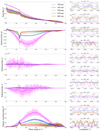 |
Fig. 4 Similar to Fig. 3 but with clouds. |
| In the text | |
|
Fig. 5 RGB colors of F (top), Q (middle), and P (bottom) of the cloudy model planet as functions of phase angle α and thelongitude in the middle of the longitude range that is visible to the observer (0° longitude corresponds with the Greenwich meridian). These color plots were constructed from the F, Q, and P phase curves at 443, 550 and 670 nm as presented in Fig. 4. The horizontal black lines indicate the respective longitudes on the geographical map on the right. |
| In the text | |
Current usage metrics show cumulative count of Article Views (full-text article views including HTML views, PDF and ePub downloads, according to the available data) and Abstracts Views on Vision4Press platform.
Data correspond to usage on the plateform after 2015. The current usage metrics is available 48-96 hours after online publication and is updated daily on week days.
Initial download of the metrics may take a while.