© ESO 2020

1. Introduction

The Galilean satellites are the four biggest moons of Jupiter, discovered by Galileo Galilei in 1610. Ordered with respect to their distance from Jupiter, they are: Io (1), Europa (2), Ganymede (3), and Callisto (4). In 1798, Laplace observed that the mean motions of Io, Europa, and Ganymede are in 4:2:1 commensurability. This configuration is made of two 2:1 two-body mean-motion resonances involving the couples Io–Europa and Europa–Ganymede. Using λ_i to denote the mean longitude of the ith satellite and ϖ_i its longitude of pericenter, we currently have

$$\begin{array}{c}\hfill \begin{array}{cc}\hfill {\lambda }_1-2{\lambda }_2+{\varpi }_1& \sim 0,\hfill \\ \hfill {\lambda }_1-2{\lambda }_2+{\varpi }_2& \sim \pi ,\hfill \\ \hfill {\lambda }_2-2{\lambda }_3+{\varpi }_2& \sim 0,\hfill \end{array}\end{array}$$(1)

where ∼ stands for “closely oscillates around”. Combining the last two relations, we obtain:

$$\begin{array}{c}\hfill {\lambda }_1-3{\lambda }_2+2{\lambda }_3\sim \pi ,\end{array}$$(2)

which involves the mean longitudes of all three satellites. This relation is commonly known as the “Laplace resonance”. Moreover, from the first two relations in Eq. (1), we can note that

$$\begin{array}{c}\hfill {\varpi }_1-{\varpi }_2\sim \pi ,\end{array}$$(3)

which implies that the orbits of Io and Europa are anti-aligned.

The orbits of regular satellites in the Solar System are generally the result of billions of years of dynamical evolution. Tidal forces between the satellites and their host planet produce dissipative effects that lead to a radial migration of the satellites over long timescales. Tidal dissipation in the Galilean satellites is the source of spectacular phenomena like the volcanism on the surface of Io (Peale et al. 1979), or the preservation of oceans of liquid water under the icy crust of Europa (Cassen et al. 1979) and probably Ganymede.

The formation of resonant configurations between satellites remained a mystery for a long time, until Goldreich (1965) put forward the idea of resonance capture through dissipative migration. Numerous works further studied this mechanism and its application to the satellites of Jupiter and Saturn, confirming the extreme importance of tidal dissipation in their long-term evolution (see e.g., Sinclair 1972, 1975; Greenberg 1973). More detailed scenarios were then developed for the Galilean satellites. Yoder (1979) and Yoder & Peale (1981) suggested that the migration of Io has always been faster than the migration of the other Galilean satellites; as a result, Io first captured Europa into mean-motion resonance, which sped up its migration and led to the subsequent capture of Ganymede. These latter authors estimated the respective probabilities of each resonance capture, and deduced lower and upper bounds for the tidal dissipation within Jupiter. Tittemore (1990) showed that the establishment of the Laplace resonance has probably been preceded by a chaotic phase in which the eccentricities of Europa and Ganymede increased dramatically. This induced a high tidal friction within the two bodies, which could explain why Ganymede and Callisto have very different surface properties. The same scenario was proposed by Malhotra (1991) and Showman & Malhotra (1997), who showed that the chaotic phase was most likely due to the crossing of three-body mean-motion resonances between Io, Europa, and Ganymede (contrary to what had first been announced by Tittemore 1990). They used this argument to obtain refined bounds for the dissipation parameters.

Other works suggest that the Laplace resonance settled during the formation of the Galilean satellites. Greenberg (1982) conjectured that the satellites were originally in deep resonance and that they are currently evolving out of resonance. In this scenario, the forced eccentricities of the satellites were initially much higher, with a consequent stronger tidal friction within all three resonant moons. Greenberg (1987) found a path of stable configurations leading from the current configuration of the Laplace resonance back to deeper resonant states. Forced to follow this path because of tidal dissipation, the Laplace angle would then have passed through asymmetric equilibria (i.e., different from 0 or π). Nevertheless, this scenario gives no information about how primordial the Laplace resonance is. According to Peale & Lee (2002), the Laplace resonance could have settled during the formation of the satellites in the circumjovian disk as a result of differential migration. Following the scenario depicted by Canup & Ward (2002), Ganymede underwent the faster Type-I migration because of its larger mass. Moving toward Jupiter, it first captured Europa in resonance, followed by Io, and this process happened relatively quickly (about 10⁵ years). After the dissipation of the disk, the satellites then reached their current state by tidal dissipation.

The future evolution of the Galilean satellites has received little attention so far. Over short and medium timescales (up to 10⁵ years), the stability of the Laplace resonance has been confirmed by Musotto et al. (2002) and Celletti et al. (2019), however little is known about its stability as a result of tidal dissipation over long timescales. It is not clear whether new reorganizations of the orbits of the moons are to be expected, as found for instance in exoplanetary systems (Batygin & Morbidelli 2013; Pichierri et al. 2019). Because of the mean-motion resonances in Eqs. (1) and (2), the strong dissipative effects acting on Io (Lainey et al. 2009) are redistributed among Europa and Ganymede. This implies that the satellites still migrate today, and that important events like the ones that occurred in the past may happen in the future. In particular, Callisto is not currently involved in any mean-motion resonance, which leads us to the question of whether or not the dissipation could ever make it cross a resonance with another Galilean satellite. Since the tidal dissipation produces an outward migration of Io, Europa, and Ganymede (Fuller et al. 2016), the first important resonance that could be encountered is the 2:1 commensurability between Callisto and Ganymede. From numerous studies of other moons (e.g., Tittemore & Wisdom 1990; Meyer & Wisdom 2008) and exoplanets (e.g., Batygin 2015; Charalambous et al. 2018), we know that a large variety of outcomes are possible, even including the ejection of one satellite (e.g., Polycarpe et al. 2018).

In this article, we aim to measure the stability of the Laplace resonance over a billion-year timescale under the effects of tidal dissipation. We also aim to determine the possible outcomes of the resonant encounter with Callisto and to quantify its capture probability.

Starting with the works of Lagrange and Laplace, the first comprehensive theories of the orbital dynamics of the Galilean satellites were meant to reproduce their current motion with a high accuracy. These theories were first analytical (e.g., Souillart 1880; de Sitter 1909), but they are now replaced by purely numerical models, mainly used for ephemerides purposes (e.g., Lainey et al. 2004a,b). Such models are extremely accurate but very computationally demanding. Even though some authors do adopt a purely numerical approach for moderately long timescales (Musotto et al. 2002), the capabilities of such simulations remain way below the billions of years required by our study, especially when it comes to drawing a statistical picture of a chaotic event. Moreover, due to the chaotic nature of the dynamics and the finite-precision arithmetic of computers, it is not possible to obtain a precise orbital solution after a few thousand years. We must instead focus on the essential elements of the dynamics, which is the purpose of secular (i.e., averaged) theories.

Lari (2018) recently presented an averaged model that was shown to describe the orbital dynamics of the Galilean satellites with unprecedented precision, while keeping the advantage of being much faster than direct numerical integration; the model also includes tidal dissipation. This model is therefore an excellent starting point for our study, even though it requires some rearrangements: mainly the introduction of the suitable resonant terms.

The paper is structured as follows. In Sect. 2, we introduce the dynamical model used to integrate the motions of the Galilean satellites. In Sect. 3, we describe our numerical experiments and analyze the outcomes of the simulations. In Sect. 4, we discuss the stability of the Laplace resonance and the variety of mean-motion resonances in which Callisto can be captured. In Sect. 5, we examine the robustness of our findings in view of the modeling of energy dissipation. Finally, we summarize our results in Sect. 6.

2. Dynamical model

For the purpose of the present study, several improvements have been made to the model of Lari (2018). Firstly, no Laplace coefficient is kept constant through time, and the equations of motion now include the partial derivatives of all Laplace coefficients. This ensures the validity of the model even if the ratios of semi-major axes vary substantially. Secondly, the orbit and obliquity of Jupiter are now allowed to vary with time according to a predefined solution. Using an appropriate evolution, the model is therefore valid over billions of years. Finally, the solar terms have been developed in Legendre polynomials and the expansion over the inclination of the Sun has been suppressed. This way, the solar contribution is more accurate (it is valid for any value of the obliquity of the planet), and numerous Laplace coefficients are no longer needed, allowing us to speed up the computations.

We also improved the implementation of the model. In particular, the integration coordinates have been changed, making the program more versatile, and a new algorithm has been implemented to compute the Laplace coefficients and their derivatives, making use of the Chebyshev interpolation. It is faster than before and accurate to machine precision. This way, we are assured that no numerical error other than round-off can add up to the truncation level inherent to the dynamical model. Below, we reiterate the basic components of the model of Lari (2018) and highlight its modifications.

2.1. Hamiltonian function

The Hamiltonian function describing the long-term orbital dynamics of the Galilean satellites can be written

$$\begin{array}{c}\hfill \mathcal{H}={\mathcal{H}}_0+\epsilon {\mathcal{H}}_1,\end{array}$$(4)

where the unperturbed part is a sum of Keplerian Hamiltonian functions:

$$\begin{array}{c}\hfill {\mathcal{H}}_0=-{\displaystyle \sum _{i=1}^N}\frac{\mathcal{G}{m}_0{m}_i}{2a_i},\end{array}$$(5)

and the perturbation can be decomposed into

$$\begin{array}{c}\hfill \epsilon {\mathcal{H}}_1={\mathcal{H}}_{}\text{J}+{\mathcal{H}}_{}\text{M}+{\mathcal{H}}_{\odot }+{\mathcal{H}}_{}\text{I}.\end{array}$$(6)

In these expressions, the index i runs over all satellites (N = 4). 𝒢 is the gravitational constant, m_i and a_i are the mass and the semi-major axis of the ith satellite, and m₀ is the mass of Jupiter. A parameter ε ≪ 1 is used here to stress that εℋ₁ is small with respect to ℋ₀ (the explicit small parameters of each part of εℋ₁ are given below). We choose an equatorial reference frame, with the third axis oriented along the spin of Jupiter and the first axis directed towards its equinox (i.e., towards the ascending node of the Sun as seen in a Jovicentric reference frame).

The term ℋ_J in Eq. (6) is due to the nonsphericity of Jupiter. We consider that Jupiter has rotational and north–south symmetries, which is very close to reality (Iess et al. 2018; Serra et al. 2019), and we use R_J to denote its equatorial radius. Up to second order in the eccentricity and inclination of the satellites, and up to fourth order in the ratio R_J/a_i, the Hamiltonian ℋ_J can be written

$$\begin{array}{cc}\hfill {\mathcal{H}}_{}\text{J}& ={\displaystyle \sum _{i=1}^N}\frac{\mathcal{G}{m}_0{m}_i}{a_i}[J_2{\left(\frac{R_{}\text{J}}{a_i}\right)}^2\frac{1}{4}(-2-3e_i^2+12s_i^2)\hfill \\ \hfill & +J_4{\left(\frac{R_{}\text{J}}{a_i}\right)}^4\frac{3}{8}(1+5e_i^2-20s_i^2)],\hfill \end{array}$$(7)

where J₂ and J₄ are the zonal gravity harmonics of Jupiter, e_i is the eccentricity of the ith satellite, I_i its inclination, and s_i ≡ sin(I_i/2).

The term ℋ_M in Eq. (6) is due to the mutual gravitational attraction between the satellites. It can be further decomposed into a secular and a resonant part:

$$\begin{array}{c}\hfill {\mathcal{H}}_{}\text{M}={\mathcal{H}}_{}{\text{M}}^{(\text{sec})}+{\mathcal{H}}_{}{\text{M}}^{(\text{res})}.\end{array}$$(8)

Up to second order in the eccentricity and inclination of the satellites, the secular part can be written

$$\begin{array}{cc}\hfill {\mathcal{H}}_{}{\text{M}}^{(\text{sec})}& =-{\displaystyle \sum _{1⩽i<j⩽N}}\frac{\mathcal{G}{m}_i{m}_j}{a_j}(f_1+f_2(e_i^2+e_j^2)-\frac{1}{2}{f}_{14}(s_i^2+s_j^2)\hfill \\ \hfill & +f_{10}{e}_i{e}_{j}cos({\varpi }_j-{\varpi }_i)\hfill \\ \hfill & +f_{14}{s}_i{s}_{j}cos({\mathrm{\Omega }}_j-{\mathrm{\Omega }}_i)),\hfill \end{array}$$(9)

where ϖ_i is the longitude of perihelion of the ith satellite, Ω_i is its longitude of ascending node, and the f_k functions are combinations of Laplace coefficients that depend on a_i/a_j <  1 (see e.g., Murray & Dermott 2000). While the three inner satellites drift outwards due to tidal dissipation, the first low-order mean-motion resonance reached involving Callisto and another Galilean satellite is the 2:1 resonance with Ganymede. This means that after some time of evolution, the corresponding harmonics cannot be considered as fast angles (contrary to evolution close to the present time considered by e.g., Lari 2018). Accordingly, up to second order in the eccentricity and inclination of the satellites, the resonant part of the averaged mutual perturbations is:

$$\begin{array}{cc}\hfill {\mathcal{H}}_{}{\text{M}}^{(\text{res})}& ={\displaystyle \sum _{ij=(12,23,34)}}[\frac{{\beta }_i{n}_i{a}_i{\beta }_j{n}_j{a}_j}{m_0}{e}_{j}cos({\lambda }_i-2{\lambda }_j+{\varpi }_j)\hfill \\ \hfill & -\frac{\mathcal{G}{m}_i{m}_j}{a_j}(f_{27}{e}_{i}cos(2{\lambda }_j-{\lambda }_i-{\varpi }_i)\hfill \\ \hfill & +f_{31}{e}_{j}cos(2{\lambda }_j-{\lambda }_i-{\varpi }_j)\hfill \\ \hfill & +f_{45}{e}_i^{2}cos(4{\lambda }_j-2{\lambda }_i-2{\varpi }_i)\hfill \\ \hfill & +f_{53}{e}_j^{2}cos(4{\lambda }_j-2{\lambda }_i-2{\varpi }_j)\hfill \\ \hfill & +f_{49}{e}_i{e}_{j}cos(4{\lambda }_j-2{\lambda }_i-{\varpi }_i-{\varpi }_j)\hfill \\ \hfill & -\frac{1}{2}{f}_{62}{s}_i^{2}cos(4{\lambda }_j-2{\lambda }_i-2{\mathrm{\Omega }}_i)\hfill \\ \hfill & -\frac{1}{2}{f}_{62}{s}_j^{2}cos(4{\lambda }_j-2{\lambda }_i-2{\mathrm{\Omega }}_j)\hfill \\ \hfill & +f_{62}{s}_i{s}_{j}cos(4{\lambda }_j-2{\lambda }_i-{\mathrm{\Omega }}_i-{\mathrm{\Omega }}_j))],\hfill \end{array}$$(10)

where λ_i is the mean longitude of the ith satellite, β_i = m₀m_i/(m₀ + m_i), and $n_i^2{a}_i^3={\mu }_i=\mathcal{G}(m_0+m_i)$. The first term is the indirect part of the perturbation (see Appendix A), whose expression was not explicitly given by Lari (2018). The terms with indexes (i, j) = (3, 4) correspond to the 2:1 resonance between Ganymede and Callisto, which is absent from Lari (2018).

The term ℋ_⊙ in Eq. (6) is due to the gravitational attraction of the Sun. Since the Sun is much farther away from Jupiter than the satellites, it is convenient to expand its perturbation in Legendre polynomials. This way, we can avoid any expansion with respect to the Sun’s inclination (Laskar & Boué 2010), meaning that the expression remains valid for any value of the obliquity of the planet considered. We write a_⊙ the semi-major axis of the Jovicentric orbit of the Sun. Up to fourth order in the ratio a_i/a_⊙, the perturbation from the Sun can be written

$$\begin{array}{cc}\hfill {\mathcal{H}}_{\odot }& ={\displaystyle \sum _{i=1}^N}\frac{\mathcal{G}{m}_{\odot }{m}_i}{a_{\odot }}[{\left(\frac{a_i}{a_{\odot }}\right)}^2(C_1^{\odot }+C_2^{\odot }(e_i^2-4s_i^2)\hfill \\ \hfill & +C_3^{\odot }{s}_i^{2}cos(2{\mathrm{\Omega }}_i)+C_4^{\odot }{s}_i^{2}sin(2{\mathrm{\Omega }}_i)\hfill \\ \hfill & +\frac{5}{4}{C}_3^{\odot }{e}_i^{2}cos(2{\varpi }_i)+\frac{5}{4}{C}_4^{\odot }{e}_i^{2}sin(2{\varpi }_i)\hfill \\ \hfill & +C_5^{\odot }{s}_{i}cos{\mathrm{\Omega }}_i+C_6^{\odot }{s}_{i}sin{\mathrm{\Omega }}_i)\hfill \\ \hfill & +{\left(\frac{a_i}{a_{\odot }}\right)}^3(C_7^{\odot }{e}_{i}cos{\varpi }_i+C_8^{\odot }{e}_{i}sin{\varpi }_i)\hfill \\ \hfill & +{\left(\frac{a_i}{a_{\odot }}\right)}^4{C}_9^{\odot }],\hfill \end{array}$$(11)

where the coefficients $C_1^{\odot }-C_9^{\odot }$ are known functions of the time that only depend on the orbital elements of the Sun, including its mean longitude (see Appendix A). For each degree in a_i/a_⊙, the order of the expansion in e_i, s_i, and the Sun’s eccentricity has been adjusted in such a way that all neglected terms have the same order of magnitude.

The term ℋ_I in Eq. (6) is due to inertial forces. This perturbation was not present in Lari (2018) because the obliquity of Jupiter and its orbit around the Sun were considered fixed. If the obliquity and orbit of Jupiter are considered to vary with time (and they do vary over long timescales), the reference system attached to Jupiter’s equator is not inertial anymore. This means that additional accelerations apply to the satellites, like the centrifugal or Coriolis terms. As shown in Appendix A, the noninertial nature of the reference frame can be taken into account by redefining the canonical coordinates used, leading to the following expression:

$$\begin{array}{cc}\hfill {\mathcal{H}}_{}\text{I}& ={\displaystyle \sum _{i=1}^N}{\beta }_i\sqrt{{\mu }_i{a}_i}[-{\mathrm{\Theta }}_z(1-2s_i^2-\frac{e_i^2}{2})\hfill \\ \hfill & +2{\mathrm{\Theta }}_y{s}_{i}cos{\mathrm{\Omega }}_i-2{\mathrm{\Theta }}_x{s}_{i}sin{\mathrm{\Omega }}_i],\hfill \end{array}$$(12)

where Θ = (Θ_x, Θ_y, Θ_z)^T is the instantaneous rotation vector of our noninertial reference frame as measured in an inertial reference frame (here, the J2000 ecliptic and equinox). The explicit expression of Θ in terms of the orbital elements and obliquity of Jupiter is given in Appendix B. It is zero if the orbit and obliquity of Jupiter are fixed in time.

In order to express the equations of motion, we need to choose a set of canonical coordinates. We start from the modified Delaunay canonical coordinates:

$$\begin{array}{c}\hfill \{\begin{array}{cc}\hfill L_i& ={\beta }_i\sqrt{{\mu }_i{a}_i}\hfill \\ \hfill G_i& ={\beta }_i\sqrt{{\mu }_{i}a}(1-\sqrt{1-e_i^2})\hfill \\ \hfill H_i& ={\beta }_i\sqrt{{\mu }_i{a}_i(1-e_i^2)}(1-cos{I}_i)\hfill \end{array}\text{and}\{\begin{array}{cc}\hfill {\ell }_i& ={\lambda }_i\hfill \\ \hfill g_i& =-{\varpi }_i\hfill \\ \hfill h_i& =-{\mathrm{\Omega }}_i\hfill \end{array},\end{array}$$(13)

where uppercase characters are the momenta, and lowercase characters are their conjugate angles¹. Since our Hamiltonian function is truncated at second order in eccentricity and inclination, we use the following relations:

$$\begin{array}{c}\hfill e_i=\sqrt{\frac{2G_i}{L_i}}+\mathcal{O}\left(e_i^3\right),s_i=\sqrt{\frac{H_i}{2L_i}}+\mathcal{O}\left(e_i^2{s}_i\right),\end{array}$$(14)

and neglect the remainders. We get rid of the coordinate singularities at e_i = 0 and s_i = 0 by the use of rectangular canonical coordinates:

$$\begin{array}{c}\hfill \{\begin{array}{cc}\hfill x_i& =\sqrt{2G_i}cos{g}_i\hfill \\ \hfill u_i& =\sqrt{2H_i}cos{h}_i\hfill \\ \hfill \end{array}\text{and}\{\begin{array}{cc}\hfill y_i& =\sqrt{2G_i}sin{g}_i\hfill \\ \hfill v_i& =\sqrt{2H_i}sin{h}_i\hfill \\ \hfill \end{array}.\end{array}$$(15)

Finally, we introduce the resonant canonical coordinates by replacing L_i and ℓ_i with

$$\begin{array}{c}\hfill \{\begin{array}{cc}\hfill {\mathrm{\Gamma }}_1& =L_1\hfill \\ \hfill {\mathrm{\Gamma }}_2& =2L_1+L_2\hfill \\ \hfill {\mathrm{\Gamma }}_3& =4L_1+2L_2+L_3\hfill \\ \hfill {\mathrm{\Gamma }}_4& =8L_1+4L_2+2L_3+L_4\hfill \\ \hfill \end{array}\text{and}\{\begin{array}{cc}\hfill {\gamma }_1& ={\lambda }_1-2{\lambda }_2\hfill \\ \hfill {\gamma }_2& ={\lambda }_2-2{\lambda }_3\hfill \\ \hfill {\gamma }_3& ={\lambda }_3-2{\lambda }_4\hfill \\ \hfill {\gamma }_4& ={\lambda }_4\hfill \\ \hfill \end{array}.\end{array}$$(16)

The generic form of these coordinates makes it easy to add or remove one satellite for test purposes.

Since the Hamiltonian function has been averaged over short-period terms, it does not depend on γ₄. This makes Γ₄ a constant of motion in the conservative case. The other variables evolve according to Hamilton’s equations. The total Hamiltonian function in Eq. (4) explicitly depends on time through the coefficients $C_1^{\odot }-C_9^{\odot }$, and through the vector Θ. Both are functions of the obliquity and orbit of Jupiter. The orbital evolution of Jupiter is taken from state-of-the-art secular theories (Laskar 1990) combined with the INPOP17a modern ephemerides². A solution for the secular dynamics of Jupiter’s spin-axis is obtained numerically. The resulting orbital and rotational solutions are put into the form of quasi-periodic series, allowing for extremely fast function evaluations. More details about how these solutions are built can be found in Appendix B.

The use of an averaged model allows us to greatly speed up the numerical integrations. The accuracy of the numerical integration can be checked by monitoring the value of the Hamiltonian function in Eq. (4), when considering a fixed orbit and obliquity for Jupiter and no dissipation. Using the numerical integrator of Everhart (1985) refined using the tips given by Rein & Spiegel (2015) ³, we found that a constant step size of 11 days is a good compromise (compared to a step size of less than one hour, which would be required in a nonaveraged model).

2.2. Tidal dissipation

Tides are differential gravitational forces acting on an extended body. Their main effect is to raise two tidal bulges along the direction between the body that generates them and the one that is exposed to their effects. This redistribution of mass induces an additional gravitational field around the deformed body, which is proportional to the Love number k₂ (Darwin 1880; Love 1909; Kaula 1964). For realistic bodies, the response to the tidal perturbation is not immediate but has a time delay, which results in a shift of the tidal bulges of a certain angle δ (see e.g., MacDonald 1964; Singer 1968; Mignard 1979) accompanied by a loss of energy due to internal friction. Both δ and k₂ depend on the interior structure of the body and its rheology (e.g., Efroimsky & Makarov 2013; Boué et al. 2016, 2019). The angle δ is related to the quality factor Q (MacDonald 1964), which is the amount of orbital energy over the dissipated energy per orbit due to tidal friction. The smaller the value of Q, the larger the dissipation inside the tidally deformed body. The value of this parameter can go from tens to hundreds for terrestrial bodies and from thousands to millions for gas giants. For an overview of energy dissipation in the Solar System, see Goldreich & Soter (1966). More recently, Ferraz-Mello (2013) developed a new theory of dynamical tides based on a simple rheophysical model of the bodies. In this model, phase lags (and therefore Q) are not ad hoc quantities designed to model the delayed response to the tides, but they are determined from the solutions of the equations.

For the aim of this work, we are interested in the long-term dynamical effects of the tidal forces. From Kaula (1964) and Peale & Cassen (1978), we know that for a couple formed by a planet and a synchronous satellite i, tides cause a secular variation of the satellite’s semi-major axis a_i, eccentricity e_i, and inclination I_i (see also Ferraz-Mello et al. 2008; Boué & Efroimsky 2019). However, no inclination-type resonance enters into play for the Galilean satellites nowadays or during the resonant encounter with Callisto (this is verified in Sect. 3.). For this reason, we can neglect the tidal effects on the orbital inclinations: if included, the dissipation would simply damp their already low values, making their contribution to the dynamics even more marginal. The variation of the semi-major axis and the eccentricity of a satellite due to the tidal dissipation can be described by the following formulas:

$$\begin{array}{cc}\hfill {\dot{a}}_i& =\frac{2}{3}{c}_i(1-(7D_i-\frac{51}{4})e_i^2)a_i,\hfill \end{array}$$(17)

$$\begin{array}{cc}\hfill {\dot{e}}_i& =-\frac{1}{3}{c}_i(7D_i-\frac{19}{4})e_i;\hfill \end{array}$$(18)

for anelastic tides, where, using the notation of Malhotra (1991),

$$\begin{array}{c}\hfill \begin{array}{cc}& c_i=\frac{9}{2}{\left(\frac{k_2}{Q}\right)}_{0,i}\frac{m_i}{m_0}{\left(\frac{R_{\mathrm{J}}}{a_i}\right)}^5{n}_i,\hfill \\ \hfill & D_i={\left(\frac{k_2}{Q}\right)}_i{\left(\frac{Q}{k_2}\right)}_{0,i}{\left(\frac{R_i}{R_{\mathrm{J}}}\right)}^5{\left(\frac{m_0}{m_i}\right)}^2;\hfill \end{array}\end{array}$$(19)

with R_i being the radius of the satellite. The ratios (k₂/Q)_i and (k₂/Q)_0, i are the dissipative parameter of the ith satellite and the dissipative parameter of the planet at the orbital frequency of the ith satellite, respectively. Indeed, from Fuller et al. (2016) and Lainey et al. (2017), we know that tidal dissipation within a planet can strongly depend on the satellite that raises the tides.

In the case of the couple Jupiter–Io, the most reliable estimate of the dissipative parameters was obtained by Lainey et al. (2009), who fitted a complete numerical model to astrometric observations taken from 1891 to 2007. The orbit determination revealed a strong energy dissipation within Io and Jupiter, with values:

$$\begin{array}{c}\hfill \begin{array}{cc}& {(k_2/Q)}_1=(1.5\pm 0.3)\times {10}^{-2},\hfill \\ \hfill & {(k_2/Q)}_{0,1}=(1.1\pm 0.2)\times {10}^{-5}.\hfill \\ \hfill \end{array}\end{array}$$(20)

Solely the dissipation in the couple Jupiter–Io has been estimated so far because tidal forces are larger for satellites that are closer to the planet.

As Io, Europa, and Ganymede are locked in mean-motion resonance, they adiabatically follow the slow drift of the resonance center due to the dissipation (this is verified in Sect. 3). This means that their ratios of semi-major axes remain approximately constant during the evolution, such that the 4:2:1 commensurability is maintained, and therefore we always have

$$\begin{array}{c}\hfill \frac{{\dot{a}}_2}{{\dot{a}}_1}{|}_{}\text{res}\approx \frac{a_2}{a_1}\approx 1.6\text{and}\frac{{\dot{a}}_3}{{\dot{a}}_1}{|}_{}\text{res}\approx \frac{a_3}{a_1}\approx 2.5.\end{array}$$(21)

Because of the mean-motion resonance, we do not expect values for (k₂/Q)_0, 2 and (k₂/Q)_0, 3 much different from the one observed for Io. Therefore, a high upper bound for the drift of the semi-major axes of Europa and Ganymede due to their intrinsic tidal dissipation can be obtained by assuming that they have the same dissipation parameters as Io, or similar. From Eq. (17), and assuming the same values as in Eq. (20), the effect of the respective tides of Europa and Ganymede on their semi-major axes is

$$\begin{array}{c}\hfill \frac{{\dot{a}}_2}{{\dot{a}}_1}{|}_{}\text{dis}\approx 0.04\text{and}\frac{{\dot{a}}_3}{{\dot{a}}_1}{|}_{}\text{dis}\approx 0.01.\end{array}$$(22)

These drifts are much smaller than the ones imposed by the resonant link (compare with Eq. (21)). Their contribution is even smaller than the error bars coming from the uncertainty of (k₂/Q)_0, 1 and (k₂/Q)₁. Consequently, we can safely neglect the contribution of Europa and Ganymede to the energy dissipation, and only consider the contribution from Io.

The dissipation parameters of Callisto are even less constrained, and Callisto is currently not involved in any mean-motion resonance. However, considering again the same dissipation parameters as Io, we obtain

$$\begin{array}{c}\hfill \frac{{\dot{a}}_4}{{\dot{a}}_1}{|}_{}\text{dis}\approx 0.0003.\end{array}$$(23)

This very small ratio shows that a dramatically high (and improbable) value of (k₂/Q)_0, 4 would be needed in order for Callisto to reach a migration rate comparable to those of Io, Europa, and Ganymede. In other words, Callisto can be considered as almost stationary with respect to the migration rates of the other moons. Consequently, we also neglect its contribution to the energy dissipation.

As seen above, the approximation of only considering the tidal dissipation generated between Io and Jupiter is justified by the many orders of magnitude that separate its level for Io and for the other Galilean satellites. Moreover, no estimate of the dissipation parameters has been obtained yet from observations for satellites other than Io (neither from astrometry nor from space missions). Therefore, instead of exploring a range of ad hoc values for these unknown parameters, we prefer to neglect them, taking advantage of their small impact on the dynamics. This approach has already been used for instance by Deienno et al. (2014); it reduces the parameter space to explore, helping us to develop a clear understanding of the simplified dynamics before any investigation of the extra level of detail that would be provided by more realistic models. In any case, underestimating the tidal dissipation in the system would mainly change the timescale of the long-term evolution of the satellites, and not its qualitative behavior (see Sect. 5 for more details).

Nevertheless, it should be noted that neglecting the energy dissipation between Jupiter and Europa, Ganymede, and Callisto also suppresses the direct damping of their eccentricities presented in Eq. (18). The eccentricity of Europa is almost entirely forced today ($e_2^{\text{forced}}\approx 0.010$ and $e_2^{\text{free}}\approx 0.000$, see Sinclair 1975) while the eccentricity of Ganymede only contains a small free component to be damped ($e_3^{\text{forced}}\approx 0.0010$ and $e_3^{\text{free}}\approx 0.0005$, see Sinclair 1975; Noyelles & Vienne 2007). Callisto is the only Galilean satellite currently possessing a substantial free eccentricity ($e_4^{\text{forced}}\approx 0.0002$ and $e_4^{\text{free}}\approx 0.0071$, see Noyelles & Vienne 2007), but considering its large distance from Jupiter, its damping for realistic values of the dissipation parameter (k₂/Q)₄ is quite small even during the gigayear timescale spanned by our numerical simulations (decrease of about 0.0010 in 1.5 Gyr assuming (k₂/Q)₄ = 10⁻³).

Since they have been directly estimated from observations, the values of the dissipative parameters given in Eq. (20) can be considered as instantaneous quantities. More generally, it is well known that each quality factor Q is a function of the tidal frequency χ, which is forced to change because of the migration of the satellite. Mignard (1979) proposed that Q = Δtχ⁻¹, assuming a constant tidal time-lag Δt. More recently, Ferraz-Mello (2013) showed that, in the pseudo-synchronous approximation, Q ∝ χ⁻¹ for inviscid bodies, while Q ∝ χ for high-viscosity bodies. Between these extreme cases, Efroimsky & Lainey (2007) noted that a constant value of Q is more realistic according to planetary interior models, at least for terrestrial bodies. Moreover, these latter authors reiterated the fact that Q depends on the temperature of the body as well, and they presented a more general model in which

$$\begin{array}{c}\hfill Q=(ϵ\chi ){}^{\beta },\end{array}$$(24)

where ϵ is a function of the temperature of the body and β is a parameter encompassing the response of the dissipation to the tidal frequency. For terrestrial bodies, Efroimsky & Lainey (2007) predicted values of β ranging from 0.2 to 0.4. Furthermore, Ojakangas & Stevenson (1986) and Hussmann & Spohn (2004) showed that Io could suffer from temperature variation cycles with a period of about 100 Myr. This would periodically change its quality factor Q, as well as its forced eccentricity. From these results, it appears that the development of a realistic frequency-dependent model of tidal dissipation would require the understanding of internal processes taking place inside the Galilean satellites. This is far beyond the scope of the present article.

Fortunately, at the level of generality required by our exploratory study, simple arguments show that there is no need for such refined models. It can be easily shown that the migration of Io needed for Ganymede to reach the 2:1 mean-motion resonance with Callisto (so that all four satellites are in a 2:1 chain of period ratios) only amounts to changing a₁ by a factor 1.1. The frequency of the tides raised on Jupiter by Io is equal to:

$$\begin{array}{c}\hfill {\chi }_{0,1}=2(w-n_1),\end{array}$$(25)

where w is the spin velocity of Jupiter. By multiplying a₁ by a factor 1.1, we obtain that χ_0, 1 changes by a factor of about 1.04 only. Likewise, the frequency of the tides raised on Io by Jupiter is equal to χ₁ = n₁, which changes by a factor of about 0.87 when a₁ is multiplied by 1.1. Consequently, even using the extreme values of β = ±1 for the frequency dependence of Q (see Eq. (24)), we find that in both cases, the variations of Q remain smaller than the uncertainties of its current value, quoted in Eq. (20). As can be seen in Sect. 3, this remains true over the whole duration of our numerical integrations. For this reason, the use of a refined frequency-dependent tidal model appears quite unnecessary in the context of our study. Therefore, we choose to use constant values for the dissipative parameters (k₂/Q)₁ and (k₂/Q)_0, 1 obtained from their estimates given in Eq. (20).

Because of the adiabatic nature of the tidal dissipation, accounting for the time dependency of k₂/Q would mostly change the timing of the resonant encounter with Callisto and hardly its topological features. Only extremely different dissipation scenarios could make the orbits vary in such a way as to transform the topology of the encounter. This crucial point is further discussed in Sect. 5. In particular, extreme dissipation variations could be produced within Jupiter if during its migration one of the satellites reaches a resonance with an oscillation mode of the interior of Jupiter. As explained by Fuller et al. (2016), the frequencies of such oscillation modes are not fixed with time but gradually shift because of the evolution of Jupiter’s internal structure (e.g., due to its cooling). A resonance-driven dissipation peak could therefore reach the location of a satellite and then drag it along, as the satellite is forced to migrate faster following the shift of the peak. It is unknown whether this mechanism has already triggered for Io (in which case the corresponding quality factor should remain constant, imposed by the resonance), or whether it will be triggered in the future (in which case the dissipation will increase). Given our current level of ignorance, it seems reasonable to continue using constant dissipative parameters, at least in the context of this preliminary investigation of the future dynamics of the Galilean satellites.

Following Malhotra (1991) and Lari (2018), we model dissipative effects as an adiabatic process. Indeed, even though (17) and (18) are not conservative and cannot be derived from the Hamiltonian function described in Sect. 2.1, their effects are very small and act on very large time spans (millions of years), well separated from the characteristic resonant (a few years) and secular timescales (hundreds of years) of the motion of the Galilean satellites. This means that in the vicinity of any time t, the conservative dynamical system from Eq. (4) is valid, but that on greater timescales, the eccentricity and semi-major axis of Io follow the trends given in Eqs. (17) and (18). Therefore, these trends can simply be added to the dynamical equations after having converted them in terms of the canonical coordinates given in Eqs. (15) and (16).

In reality, the dissipative effects described above are so small (i.e., so well adiabatic) that we can even use a multiplying factor α to the dissipative parameters, following the approach of Malhotra (1991) and Showman & Malhotra (1997). Using a dissipative parameter α times larger implies that the migration of the satellites is α times faster, which drastically reduces the computation time. This linear acceleration law can be proven by linearizing the small semi-major drift resulting from the tidal dissipation (see Eq. (17)). This method is valid as long as the accelerated energy dissipation remains adiabatic with respect to the conservative part of the dynamics. The choice of a suitable value for α is therefore critical. By examining the characteristic timescales of the dynamics of the Galilean satellites, Malhotra (1991) set an upper limit for α below which the evolution is not distorted by the artificial acceleration. Based on this result, Malhotra (1991) and Showman & Malhotra (1997) used an acceleration factor of about 10³ in their simulations. Here, we make a more conservative choice and set α to 10². In the following sections, we give the results as a function of the physical time, which is obtained as the integration time multiplied by α. Therefore, the gigayear scale in the figures of Sect. 3 represents 10 Myr of actual integration time. The validity of this acceleration method and the quality of the adiabatic approximation is checked and further investigated in Sect. 5.

2.3. Initial conditions

We start our integration at time J2000. We use the same method as Lari (2018) in order to build suitable initial conditions for the semi-secular model: we filter the series of orbital elements taken from the Jup310 ephemerides⁴, removing the short-period harmonics. As shown by Lari (2018), integrations with our model for 100 years (about the time that ephemerides cover) are in very good agreement with the filtered series of Jup310. This means that this model very accurately reproduces the resonant and secular dynamics of the Galilean satellites. The system is then propagated forward for billions of years. The values of the parameters and of the initial conditions used in this article are given in Table 1.

3. Long-term evolution

The current configuration of the system consists in a chain of two 2:1 mean-motion resonances in the couples Io–Europa and Europa–Ganymede. From Lainey et al. (2009), we know that at present Io is moving toward Jupiter, while Europa and Ganymede move away from the planet. However, on a long timescale, the tidal dissipation results in an outward migration for all the satellites. Indeed, as shown in Fig. 1, after about 4 Myr Io stops its inward migration and starts migrating outwards. This inversion is not due to a change of sign in Eq. (17): the slow trend imposed by the tidal dissipation always remains positive. Instead, this change of direction is due to the fact that a₁ decreases and a₂ increases, meaning that the ratio a₂/a₁ changes rapidly (while remaining close to the value quoted in Eq. (21)). This shift of the resonance center between Io and Europa induces a variation of the forced values of their eccentricities (see Fig. 2). Since the eccentricity of Io decreases, dissipation in Jupiter gains importance against the one within Io (see Eq. (17)). This provides more energy to the orbit of Io and makes all three semi-major axes increase.

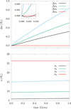Fig. 1. Variation of the satellites’ semi-major axes (Δa and a) in the first phase of the evolution. Due to the Laplace resonance, the tidal dissipation is distributed among Io, Europa, and Ganymede. As shown in the zoom-in view, Io initially migrates inward and then outward like Europa and Ganymede. Callisto does not have any secular trend.

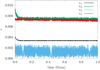Fig. 2. Variation of the satellites’ eccentricities in the first phase of the evolution. Io and Europa’s eccentricities initially decrease, and then, when a2/a1 remains almost constant, they stabilize to new values.

This current, surprising behavior of the Galilean satellites may conceal some clues about the origin of the Laplace resonance. Today, the mean-motion relations n₁ − 2n₂ and n₂ − 2n₃ increase because the satellites migrate in different directions. This increase has been reported for instance by Lainey et al. (2009). As explained in Sect. 1, it could seem to favor a primordial origin of the Laplace resonance, since the satellites would now be evolving away from deep resonance. However, this “decay” of the resonance, put forward for instance by Peale & Lee (2002), stops after a relatively short amount of time, once an equilibrium is reached between the resonant dynamics and the dissipative effects. The Laplace resonance is fully preserved. Therefore, this temporary behavior could hardly be related to a global trend pushing the system away from a primordial hypothetical state. On the contrary, it could indicate that the Laplace resonance is quite new, since it has not yet reached an equilibrium configuration. More probably, this transition could be due to cyclic variations of the dissipation parameters, periodically forcing the Laplace resonance to slightly resettle at the new equilibrium configuration. As detailed in Sect. 2.2, such variations could be due to internal processes of the planet (e.g., Burkart et al. 2014), and/or of the satellite (e.g., Ojakangas & Stevenson 1986; Hussmann & Spohn 2004). However, as pointed out by Fuller et al. (2016), we expect in the long run to observe an outward migration of all three Galilean satellites, as shown in Fig. 1. In case of cyclic variations, the constant dissipation parameters used in our model should therefore be interpreted as mean values, representative of the global trend of the system.

Using the values of the dissipative parameters from Eq. (20), we obtain that for about 1.4 Gyr from today the evolution is very stable: all the current resonances are preserved, and small differences in the initial conditions do not change the qualitative behavior of the resonant angles nor the timescale of the migration. This proves the stability of the Laplace resonance under the action of tidal dissipation over very long timescales.

However, after 1.4 Gyr, as Ganymede approaches the 2:1 mean-motion resonance with Callisto, chaotic effects show up: orbital elements suddenly change because of the exit from mean-motion resonances or the capture into new ones. From this point on, a small change in the variables (or in the model) results in a completely different evolution of the system. For this reason, we adopt a statistical approach to study the outcome of the resonant encounter. Since Callisto is initially out of any mean-motion resonance, its mean longitude (contained in the variable γ₃) at a given time can be considered as random with respect to the longitude of any other satellite in the system. As a result, a tiny error in the initial conditions of the satellites (or in the dynamical model) is transformed after 1.4 Gyr into a uniform distribution of γ₃ in [0, 2π). Hence, starting from the coordinates at 1.4 Gyr obtained from our nominal propagation, we generate a list of new initial conditions, in which γ₃ is sampled in the whole interval [0, 2π) while the other variables are kept the same. We use a sampling step of about 0.01 radians so that the total number of simulations is 628.

As a general result of our 628 simulations, Callisto always ends up captured in some mean-motion resonance. Indeed, a secular drift of its semi-major axis is triggered in all simulations, implying that the dissipative effects on Io manage to reach the orbit of Callisto through some chain of mean-motion resonances. However, at about 1.5 Gyr, our simulations split into different cases. We classify them according to the end state of the system. We discriminate between

• case A: a chain of three 2:1 two-body mean-motion resonances in the couples Io–Europa, Europa–Ganymede, and Ganymede–Callisto; and

• case B: a resonant chain including the 2:1 mean-motion resonance between Io and Europa, plus at least one pure three-body resonance.

As in Gallardo et al. (2016), a “pure” three-body resonance means that it is not the result of the sum of two-body resonances (contrary to the current configuration of Io, Europa and Ganymede). Therefore, it corresponds to the librations of a three-body resonance angle while the corresponding two-body angles circulate. For instance, if σ = σ₁ + σ₂ is a librating three-body-resonance angle, it is referred to as pure if the two-body-resonance angles σ₁ and σ₂ both circulate (two examples are given in Fig. 7). By observing the drift of semi-major axis, we can be assured that the pure three-body mean-motion resonance indeed drives the dynamics.

Cases A and B cover our whole set of 628 simulations. Within them, we can distinguish different behaviors by looking at the evolution of the resonant angles and eccentricities. The Laplace resonance that remains stable up to about 1.5 Gyr can be preserved or disrupted, as we see below. However, it is worth noting that the only angle that continues to librate in all simulations is λ₁ − 2λ₂ + ϖ₁ (although it can be temporarily excited as a result of the creation or disruption of other resonances). This means that the couple Io–Europa always remains locked in the 2:1 resonance. Indeed, Io and Europa are further away from Callisto than Ganymede and their dynamics are less perturbed by the resonant encounter. We also note that the inclination degrees of freedom appear to be unimportant in this problem: the inclinations remain low, even though we did not include any damping of their values (see Sect. 2.2), and no major inclination resonance is found to drive the dynamics in any of our 628 simulations.

3.1. Case A: two-body resonant chain

Case A is the most probable outcome (354 simulations over 628): Ganymede and Callisto enter into a 2:1 two-body mean-motion resonance, while the current resonances between Io, Europa, and Ganymede are preserved (see Eq. (1)), as well as the Laplace relation (see Eq. (2)). The mean longitudes of Ganymede and Callisto verify

$$\begin{array}{c}\hfill {\lambda }_3-2{\lambda }_4+{\varpi }_3\sim 0,\end{array}$$(26)

as shown in Fig. 3. The new resonant angle is of the first order in the masses and in the eccentricities, therefore it is a very strong term in the Hamiltonian. The angle λ₃ − 2λ₄ + ϖ₄ also happens to librate in some simulations (72 over 354), but never without Eq. (26), and this does not affect the qualitative behavior of the system.

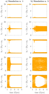Fig. 3. Typical evolution of the first-order resonant angles in case A. Column a: λ2 − 2λ3 + ϖ3 starts to librate. Column b: λ2 − 2λ3 + ϖ3 continues to circulate. See text for the definition of case A and a description of the dynamics.

The resonance between Ganymede and Callisto completes the full chain of 2:1 resonances, such that once Callisto is captured, it starts to migrate outward (see Fig. 5a). This shows that the dissipative effects acting on the orbit of Io spread to all moons and now reach Callisto. Figure 6a shows that after the crossing of the chaotic region generated by the resonant encounter, the eccentricities stabilize to new low values forced by the two-body resonances. These values remain below 0.01, similar to the ones we observe nowadays, along the whole propagation of 5 Gyr.

In most simulations ending in case A (326 over 354), another angle begins to librate:

$$\begin{array}{c}\hfill {\lambda }_2-2{\lambda }_3+{\varpi }_3\sim 0,\end{array}$$(27)

as illustrated in Fig. 3a. This is the missing relation that defines the De Sitter resonance, allowing the existence of periodic orbits for the four-body system composed of Jupiter, Io, Europa, and Ganymede (see de Sitter 1909). This additional resonance means that the longitudes of the satellites’ nodes all precess at the same rate: we have ϖ₂ − ϖ₁ ∼ π, and ϖ₃ − ϖ₂ ∼ π. This also implies that five of the six first-order resonance angles librate (we have simultaneously Eqs. (1), (26), and (27)). This is a very stable configuration: once the eccentricities are settled in their new forced values, our integrations do not show any significant change. The satellites continue to migrate outward and all the established resonances are preserved. The simultaneous Eqs. (1), (26), and (27) imply that a large number of other angles librate, including

$$\begin{array}{c}\hfill {\lambda }_1-2{\lambda }_2-{\lambda }_3+2{\lambda }_4\sim 0.\end{array}$$(28)

Like the current Laplace resonance (see Eq. (2)), this last relation is a geometrical consequence of the libration of other angles. It means that when Io and Ganymede are in conjunction, so must be Europa and Callisto, a very interesting configuration that involves all the Galilean satellites.

In a few simulations ending in case A (28 over 354), on the contrary, the angle λ₂ − 2λ₃ + ϖ₃ continues to circulate (compare Figs. 3a and 3b). In this case, we observe that the 2:1 resonance between Ganymede and Callisto can be disrupted after a few billion years (i.e., Eq. (26) is no longer verified). Indeed, λ₃ − 2λ₄ + ϖ₃ oscillates with a wider and wider amplitude until it returns to circulation, and Europa, Ganymede, and Callisto eventually end up in a pure three-body resonance. This evolution is characterized by a slow increase of Callisto’s eccentricity (see Fig. 6b), which stops once the system settles in its new configuration. However, this process is extremely slow.

3.2. Case B: Chain with a pure three-body resonance

The remaining simulations (274 over 628) show more complex evolutions involving the formation of a 4:2:1 pure three-body mean-motion resonance. Theoretically, this kind of resonance could involve the triplet Io–Europa–Ganymede, or the triplet Europa–Ganymede–Callisto, or both of them. However, the pure resonance Io–Europa–Ganymede only appears as a transitory state in our simulations (see Sect. 4.1 below). We only found one simulation in which a pure resonance Io–Europa–Ganymede seemed to have lasting effects, but due to its low statistical significance, and since the evolution of the eccentricities in this simulation does not differ much from the general case B described below, we do not emphasize it any further. All the other simulations classified in case B (273 over 274) involve a pure three-body resonance between Europa, Ganymede, and Callisto. Differently from case A, Ganymede and Callisto do not lock into the 2:1 two-body resonance (see Fig. 4), at least not immediately, but they enter into a pure three-body resonance with Europa. As before, all simulations show a drift in the semi-major axis of Callisto, which asserts its capture into resonance.

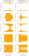Fig. 4. Typical evolution of the first-order resonant angles in case B. Column a: λ2 − 2λ3 + ϖ2 starts to circulate. Column b: λ2 − 2λ3 + ϖ2 continues to librate. See text for the definition of case B and a description of the dynamics.

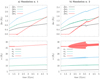Fig. 5. Typical long-term evolution of the semi-major axes (Δa and a). The bottom graphs also show the pericenter and apocenter distances, represented as a colored interval around the value of a. Left column: stable case where, after the first capture of Callisto into resonance, the system remains in the same configuration and the migration of the satellites is almost linear. Right column: unstable case where, at about 3.5 Gyr after time J2000, one of the resonances is disrupted and a new one is formed.

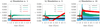Fig. 6. Typical evolution of the eccentricities in simulations where the Laplace resonance and all the current resonances are preserved. Panel a: case A with λ2 − 2λ3 + ϖ3 in libration; all the eccentricities rapidly settle to new low values. Panel b: case A with λ2 − 2λ3 + ϖ3 in circulation; Callisto’s eccentricity increases slowly as it exits its resonance with Ganymede. Panel c: case B with λ2 − 2λ3 + ϖ2 in libration; after an abrupt increase the eccentricities converge to new values.

Most simulations classified in case B (212 over 274) are characterized by the resonant angle

$$\begin{array}{c}\hfill 2{\lambda }_2-5{\lambda }_3+2{\lambda }_4+{\varpi }_3\sim \pi ,\end{array}$$(29)

and a few others (48 over 274) have

$$\begin{array}{c}\hfill {\lambda }_2-3{\lambda }_3+2{\lambda }_4\sim \pi .\end{array}$$(30)

Typical examples are given in Fig. 7. The remaining simulations classified in case B involve other three-body resonances that are not always easy to identify. The terms associated to these angles are of the second order in the masses. This means that they do not directly appear inside the Hamiltonian in Eq. (4); instead, they appear in the remainders of the Lie-series when using a perturbative approach (see e.g., Nesvorný & Morbidelli 1998). By computing these remainders, we observe that the lowest-order three-body angles result from the sum or the difference of two circulating two-body angles (see Eq. (10)). In our simplified model, such terms are at least of order two in the eccentricities. These terms are relatively small, but they are incredibly numerous; and indeed, we observe that all pure three-body resonances in our model appear when ϖ₃ − ϖ₂ and/or ϖ₄ − ϖ₃ librate, that is, when numerous combinations analogous to Eqs. (29) and (30) act together and combine their effects. This property is discussed further below.

Fig. 7. Examples of simulations in which Callisto is trapped in a pure three-body resonance. Left: a case with 2λ2 − 5λ3 + 2λ4 + ϖ3 ∼ π; right: one with λ2 − 3λ3 + 2λ4 ∼ π.

At this point, it is worth noting that in the process of eliminating short-period terms from the Hamiltonian (see Sect. 2), we eliminated many three-body resonant combinations. For example, the fast angles λ₂ − λ₃ and 2λ₃ − 2λ₄ that are absent from our model would generate a contribution to Eq. (30) of order zero in eccentricity. More generally, a complete nonaveraged dynamical model would contain more pure three-body resonances than our model. On the one hand this would increase the capture probability of Callisto (which is already 100% in our simulations), but on the other hand it could somehow alter the classification scheme that we use, especially concerning the simulations ending in case B. Therefore, the simulations presented below are not meant to be representative of every possible evolution involving pure three-body resonances. However, we highlight the fact that our results feature the same three-body inequalities as those obtained by Malhotra (1991) and Showman & Malhotra (1997). For instance, the Laplace-like resonance of these latter authors, identified by (2n₂ − n₁)/(2n₃ − n₂)≈1/2, can be rewritten as 2n₁ − 5n₂ + 2n₃ ≈ 0, which is the same relation obtained here for the three outer satellites by deriving Eq. (29). The evolution of the satellites’ eccentricities, which is described below, is also very similar.

In most simulations classified in case B (233 over 274), the resonances λ₂ − 2λ₃ + ϖ₂ and λ₁ − 2λ₂ + ϖ₂ are destroyed. The 2:1 resonance between Io and Europa is the only resonance that survives (see Eqs. (1) and (2)), while the pure three-body resonance appears. The Laplace resonance is broken, destabilized by the resonant encounter with Callisto. This transition can be slow (about 1 Gyr, as shown in Fig. 4a) or very fast (a few million years). During this transition, the eccentricities of the satellites evolve in strong correlation with the longitudes of their pericenters:

• If ϖ₂ − ϖ₃ librates, the eccentricity of Ganymede increases quickly up to about 0.04. Then the whole system stabilizes, and the three-body resonance is preserved up to the end of the five-gigayear integration (see Fig. 8a).

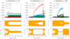
  Fig. 8. Typical evolution of the eccentricities in simulations where the Laplace resonance is disrupted. Column a: case B with ϖ2 − ϖ3 ∼ 0; all the eccentricities remain below 0.04. Column b: case B with ϖ2 − ϖ3 in circulation and ϖ3 − ϖ4 ∼ 0; the eccentricity of Callisto increases until the pure three-body resonance is disrupted. Column c: case B with ϖ2 − ϖ3 in circulation and ϖ3 − ϖ4 ∼ π; the eccentricity of Ganymede increases until the pure three-body resonance is disrupted.

• If ϖ₂ − ϖ₃ circulates, but ϖ₃ − ϖ₄ librates, the eccentricities of Ganymede and Callisto slowly increase up to large values. A similar evolution was observed by Malhotra (1991) and Showman & Malhotra (1997) before the formation of the current Laplace resonance. We observe distinct behaviors of the eccentricities according to the value around which ϖ₃ − ϖ₄ librates (see Figs. 8b and 8c). Its libration around zero produces a faster increase of the eccentricity of Callisto, while its libration around π produces a faster increase of that of Ganymede. This happens because the three-body resonant terms that dominate are not the same in both cases. This is similar to the mechanism described by Pichierri et al. (2019): as energy is gradually dissipated, the satellites adiabatically follow the resonance center, which drifts to higher and higher values of the eccentricities. However, beyond some threshold of the eccentricities, the system appears to be unstable. This is probably because the increase of the eccentricities widens neighbor resonances, which eventually overlap and destabilize the system. The pure three-body resonance is therefore disrupted and eccentricities are damped again to very small values. The satellites are then immediately captured into a new resonant configuration, which cannot be uniquely determined because of the chaotic nature of the transition. As shown in Fig. 8, these cycles can go on for billions of years.

In the remaining simulations classified in case B (40 over 274), λ₂ − 2λ₃ + ϖ₂ continues to librate (see Fig. 4b). Therefore, Europa and Ganymede remain locked in their two-body resonance and the Laplace relation (2) remains, while Callisto enters into a pure three-body resonance with Europa and Ganymede. Since the current resonances between Io, Europa, and Ganymede are preserved, the variations of their eccentricities remain moderate, as shown in Fig. 6c. The eccentricity of Callisto is the only one to suffer from a slight increment, but then it stabilizes rapidly below 0.02. For some of these simulations, we observe a slow transition to case A: after a few billion years, Ganymede and Callisto finally enter the 2:1 two-body resonance.

Throughout this section, we see that simulations classified as case B can feature a large increase of the eccentricity of Ganymede and/or Callisto (up to about 0.1). However, as illustrated in Fig. 5b, these growths are far too small to allow them to cross orbits of other satellites: this prevents any catastrophic event, such as ejections or collisions.

4. Discussion

4.1. Evolution of the Laplace resonance

Section 3 shows that the resonant encounter with Callisto can preserve the Laplace resonance between Io, Europa, and Ganymede (case A and a few simulations from case B), or destroy it (case B). More precisely, the Laplace resonance, meant as the chain between the 2:1 resonances of the couples Io–Europa and Europa–Ganymede, is preserved in 394 over 628 simulations (about 63%). In the remaining simulations, this configuration is destroyed: the angles λ₁ − 2λ₂ + ϖ₂ and λ₂ − 2λ₃ + ϖ₂ pass from libration to circulation, and the relation in Eq. (2) no longer holds.

Nonetheless, for a restricted period of time during the chaotic transitions observed in cases A and B, we found a few examples in which the two-body angles λ₁ − 2λ₂ + ϖ₂ and λ₂ − 2λ₃ + ϖ₂ start to circulate while the three-body relation (2) still holds. This means that the 4:2:1 three-body resonance between Io, Europa, and Ganymede becomes pure. This configuration generally persists for only a few hundred million years. As shown in Fig. 9, this “pure Laplace resonance” induces a peculiar evolution of the eccentricities: that of Europa shows a rapid and significant increment up to 0.06, while those of the other moons remain anchored to low values. This mechanism is similar to the one described in Sect. 3.2 (case B), which makes the eccentricities of Ganymede and Callisto increase when the three outer satellites are locked in a pure three-body resonance. This is also what Malhotra (1991) and Showman & Malhotra (1997) obtained while studying the formation of the Laplace resonance.

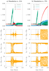Fig. 9. Examples of simulations where the three-body resonance between Io, Europa, and Ganymede becomes pure for a few hundred million years. The area confined between the two dashed black lines is the time span where λ1 − 2λ2 + ϖ2 and λ2 − 2λ3 + ϖ2 circulate, and λ1 − 3λ2 + 2λ3 librates. Left: transition to case A. Right: transition to case B.

4.2. The jungle of two- and three-body resonances

Section 3 shows that due to tidal dissipation, numerous two-body and three-body mean-motion resonances can affect the orbital dynamics of the Galilean satellites in the future. Such resonances do not appear randomly. Since they mainly depend on the period ratios among the satellites (and not much on their precession rates), it is even possible to roughly estimate their location. As Io, Europa, and Ganymede are initially tightly locked in resonance (i.e., their period ratios are fixed), the different resonances can be located as a function of Callisto’s period ratio only, for instance with respect to Ganymede. From the Hamiltonian function in Eq. (10), the only possible three-body resonances at second order of the masses are of the form

$$\begin{array}{c}\hfill \begin{array}{cc}& (n_2-2n_3)\pm (n_3-2n_4),\hfill \\ \hfill & 2(n_2-2n_3)\pm (n_3-2n_4),\hfill \\ \hfill \end{array}\begin{array}{cc}& (n_2-2n_3)\pm 2(n_3-2n_4),\hfill \\ \hfill & 2(n_2-2n_3)\pm 2(n_3-2n_4).\hfill \\ \hfill \end{array}\end{array}$$(31)

Figure 10 shows the relative locations of these resonances and the order in which they can be encountered as Io, Europa, and Ganymede migrate outwards. When taking into account the precession rates of the orbits, each of these resonances splits into a series of multiplets that partially overlap with each other, producing the chaotic evolution observed in the simulations (see Nesvorný & Morbidelli 1998; Gallardo et al. 2016). This explains why chaos appears before actually reaching the 2:1 two-body resonance between Ganymede and Callisto. However, if ϖ₃ − ϖ₄ and/or ϖ₂ − ϖ₃ oscillate with a small amplitude, many multiplets merge together (exact overlap), allowing the three-body resonance to stand on its own and produce the dynamics described in Sect. 3.2 (case B). As shown by Fig. 10, the first three-body resonance reached by the satellites is 2λ₂ − 5λ₃ + 2λ₄; this resonance is the one that we most frequently find in case B. In case A, on the contrary, the chaotic zone is crossed quickly and the satellites end up in the strong two-body mean-motion resonance.

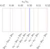Fig. 10. Location of the two-body (blue) and three-body (red) mean-motion resonances as a function of the ratio between the mean motions of Callisto and Ganymede. The dashed black line is its value at 1.4 Gyr. Tidal dissipation makes it move from left to right.

5. Significance of our results

As detailed in Sect. 2, our model inevitably relies on many simplifications. In particular, the results described in Sect. 3 are obtained using constant dissipation parameters and through a procedure of computational acceleration (see Sect. 2.2). Moreover, the statistical picture of the different dynamical outcomes is developed from a limited number of simulations, which necessarily limits its precision. All these factors are linked and impact our results in some way. Our approach can legitimately be questioned, and its range of validity needs to be investigated. This is the purpose of this section.

5.1. Acceleration factor

Even though our results are presented in Sect. 3 in terms of the real physical time t, they are obtained by applying an acceleration factor α = 10² to the dissipation parameters. Because of the adiabatic nature of the energy dissipation, this amounts to using an integration time-variable $\stackrel{\sim }{t}$ for the numerical computations, which is related to the physical time through $t\approx \alpha \stackrel{\sim }{t}$. As stressed in Sect. 2.2, this method is relevant only as long as the accelerated dissipation process is still adiabatic. If not, we expect spurious artifacts to appear in the dynamics. The adiabatic nature of the dissipation can be studied by varying the value of α. Indeed, the accelerated dissipation process is still adiabatic if: (i) in the regular portions of the evolution, changing α only changes the timescale; and (ii) in the chaotic portions of the evolution, changing α does not change the statistics of the outcomes.

For values spanning many orders of magnitude, Fig. 11 shows the influence of α during the first gigayear of the satellites’ evolution (regular dynamics). We only need to examine the semi-major axis and eccentricity of Io since the energy dissipation is spread through them to the whole satellite system (see Sect. 2.2). Figure 11 shows that no qualitative or quantitative change of the dynamics occurs for values of α ranging up to 10⁵: we only observe a linear contraction of the integration time-variable $\stackrel{\sim }{t}$. For α = 10⁶, on the contrary, the dynamical evolution is completely different: the eccentricity of Io undergoes an abrupt decrease followed by spurious oscillations. Indeed, for α = 10⁶ and beyond, the evolution of e₁ is more affected by the magnified dissipation than by the conservative dynamics, meaning that the adiabatic approximation fails spectacularly.

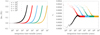Fig. 11. Evolution of the semi-major axis and eccentricity of Io with respect to the integration time-variable $\stackrel{\sim }{t}$ for different acceleration factors α. The time is given in a logarithmic scale. The duration of each integration is set so that it represents 1 Gyr of physical time t used in Sect. 3. Up to α = 105, a change of α only amounts to a linear contraction of the integration time (i.e., the curves overlap when viewed with respect to the physical time t).

As a result, the choice of α = 10² seems to be quite reliable, at least during the first portion of the evolution presented in Sect. 3, when the dynamics are regular and driven by the strong Laplace resonance. However, the chaotic transitions that follow feature very weak resonances such as pure three-body resonances. Being shallower, those resonances are associated with longer libration timescales that could endanger the adiabaticity of the accelerated energy dissipation. Although statistical analyses using α = 1 or 10 are prohibitive due to overly large computation times, a full statistical picture of the dynamical outcomes can be obtained for larger accelerations. Meaningful statistical deviations beyond a given threshold of α mean that the limit of validity of the adiabatic approximation is reached. This approach has been used for instance by Tittemore & Wisdom (1988). In order to determine this threshold, we perform 628 additional simulations for each new value of α = 10³, 10⁴, and 10⁵. We then classify them according to the outcome of the resonant encounter with Callisto, as we did in Sect. 3. For better comparison, we enrich our classification scheme as follows:

• A:

  Chain of three two-body resonances.

• B.1:

  Pure three-body resonance involving Europa, Ganymede, and Callisto.

• B.2:

  Pure three-body resonance involving Io, Europa, and Ganymede.

• C:

  The two-body resonance between Io and Europa is destroyed.

Our results are presented in 2. In order to compare them, we first need to quantify the statistical significance of their differences. Assuming that the division between outcomes amounts to a random process, the probability of obtaining k times a given outcome (e.g., case A) among n = 628 trials obeys a binomial distribution. Using p to denote the probability of obtaining case A when performing a single numerical integration, the expected number of successes is

$$\begin{array}{c}\hfill E=np,\end{array}$$(32)

with a variance equal to

$$\begin{array}{c}\hfill {\sigma }^2=np(p-1).\end{array}$$(33)

When n grows, the binomial distribution rapidly tends to a normal distribution, so that E and σ² can be interpreted in the usual way. For n = 628 and a probability p close to 0.5, the 3σ uncertainty range of the fraction of successes is about 6%. The fractions of cases A and B obtained for α = 10² and α = 10³ are therefore perfectly compatible (see Table 2). For less probable outcomes, the 3σ range is smaller: for instance, we obtain an uncertainty range of about 3% for p = 0.05. The fraction of case B.2 obtained for α = 10² and α = 10³ are therefore only marginally compatible. This indicates that for an acceleration factor α = 10³, the adiabatic approximation already slightly begins to crumple. Finally, the fractions obtained for α = 10⁴ and beyond are clearly not compatible with those obtained for smaller values of α; this means that the adiabatic approximation is not valid for such large energy dissipations. In particular, the occurrence of case C means that Io is pushed so heavily by the dissipation that even the small perturbation due to the resonant crossing of Ganymede with Callisto is able to make it escape its resonance with Europa. We also note that the number of simulations featuring a pure three-body resonance between Europa, Ganymede, and Callisto (case B.1) abruptly decreases beyond α = 10⁴ because the system has no time to explore such weak resonances before reaching the strong two-body resonance between Ganymede and Callisto (see Sect. 4.2 and Fig. 10). In contrast, the value α = 10² used throughout this article appears to be quite satisfactory.

5.2. Tidal dissipation model

As explained in Sect. 2.2, the use of constant dissipation parameters is justified by the fact that their hypothetical variations given by conventional frequency-dependent models remain below the level of uncertainty of their value. In order to explore different dissipation models, it appears therefore more sensible to continue using constant parameters and to sample their respective uncertainty ranges. Due to the adiabatic nature of the dissipation, allowing the parameters to vary would simply mean that the evolution timescales of a₁ and e₁ are not constant, but that they slowly contract or expand inside the limits given by our sampling. As shown in Sect. 5.1, the current dissipation rate could even be multiplied by 10³ in the future without threatening its adiabatic nature. For each set of constant parameters, we need to measure critical properties of the dynamics that can serve as a proxy of their effect. Since these parameters mostly modify the evolution timescale, their effects can be quantified by measuring the epoch of the resonant encounter with Callisto. Guided by Fig. 10, we arbitrarily define the beginning of the resonant encounter when the period ratio of Ganymede and Callisto exceeds 0.48.

Figure 12 shows the time of the resonant encounter obtained for a fine grid of parameters (k₂/Q)_0, 1 and (k₂/Q)₁ sampled within their uncertainties (see Eq. (20)). The encounter time is 1.5 Gyr in our nominal simulations analyzed in Sect. 3 (central cross), but we see that it can vary from about 1.2 to 1.9 Gyr. The encounter time is much more sensitive to the value of (k₂/Q)_0, 1 than to the value of (k₂/Q)₁. This is because the dissipation inside Jupiter has a dominant role in ruling the drift of the semi-major axes (see Eq. (17)), especially after the eccentricity of Io stabilizes at a lower value (see Fig. 2). As mentioned in Sect. 3, the convergence value of e₁ results from an equilibrium between the resonant dynamics and the tidal dissipation. As shown in Fig. 13, this convergence value is slightly affected by the value of the dissipative parameters sampled in their uncertainty range. This also somehow modifies the equilibrium eccentricity of Europa (see Fig. 2, where both e₁ and e₂ vary simultaneously), but not enough to produce noticeable dynamical changes during the resonant encounter with Callisto. Interestingly, the eccentricity of Io is already at its equilibrium value today if ever the dissipative parameters have values (k₂/Q)_0, 1 = 1.3 × 10⁻⁵ and (k₂/Q)₁ = 1.2 × 10⁻². However, this is at the very limit of the uncertainty range provided by Lainey et al. (2009).

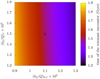Fig. 12. Time of the resonant encounter from today as a function of the values of the dissipative parameters. The axis ranges correspond to the uncertainties given by Lainey et al. (2009).

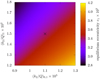Fig. 13. Equilibrium eccentricity of Io before the resonant encounter as a function of the values of the dissipative parameters. The axis ranges correspond to the uncertainties given by Lainey et al. (2009).

6. Conclusion

Tidal dissipation causes the orbits of the Galilean satellites to slowly migrate with time. Energy is mostly dissipated by the tidal interactions between Io and Jupiter, but the effects of the dissipation are then redistributed among the satellites through the Laplace resonance. Over billions of years, this produces an outward migration of Io, Europa, and Ganymede. Since it is not currently involved in any mean-motion resonance, Callisto does not yet migrate substantially. However, as Io, Europa, and Ganymede migrate outwards, Callisto is progressively reached by the 2:1 resonance with Ganymede.

In this article, we study the possible outcomes of this resonant encounter. We focus on the probability of capturing Callisto into mean-motion resonance, and on the stability of the current Laplace resonance. To this end, we used the semi-analytical model of Lari (2018), which is adjusted to take into account possible resonances between Ganymede and Callisto, and refined to support numerical integrations over a gigayear timescale. We set the duration of our numerical integrations to 5 Gyr. We assumed constant dissipation parameters, fixed to the values measured by Lainey et al. (2009). These values are still a matter of debate in the literature, but due to the adiabatic nature of the energy drift, a more detailed dissipation model would mostly change the timescale of the resonant encounter, and not its dynamical properties. The extremely accurate data expected from future space missions (JUICE, Europa Clipper), coupled with astrometric data sets, should provide a better understanding of dissipative parameters (Dirkx et al. 2017; Lari & Milani 2019).

We find that up to about 1.5 Gyr from now, the orbit of Callisto remains virtually unchanged and all the current resonances between Io, Europa, and Ganymede are preserved during their migration. However, after 1.5 Gyr, the proximity of the 2:1 mean-motion resonance between Ganymede and Callisto produces chaotic effects and a large variety of outcomes become possible. We draw a statistical picture of the dynamics based on a sample of 628 integrations.

In 56% of the cases, Callisto is captured right away into the 2:1 resonance with Ganymede (case A). The Galilean satellites therefore reach a perfect chain of two-body resonances. In the remaining 44% of the cases, a resonant chain involving all four satellites is also formed, but it includes a pure three-body 4:2:1 mean-motion resonance (case B). Apart from just one simulation, this three-body resonance involves Europa, Ganymede, and Callisto. From a statistical point of view, we expect an absolute uncertainty of a few percent in the division between cases A and B. In all our 628 simulations, Callisto remains trapped in some mean-motion resonance, which makes it migrate outwards along with the other satellites. Its capture therefore appears to be a highly probable event. This also suggests that regardless of the tidal history of the Galilean satellites, Callisto never crossed the 2:1 resonance with Ganymede in the past, otherwise it would have remained locked. Indeed, a 2:1 resonance crossing of Ganymede and Callisto without capture would require a huge migration rate, which is incompatible with the observations.

In case A, the eccentricities of all satellites settle to small values. As in the current configuration of the system, the 2:1 resonances force the eccentricities to remain small according to the precession rate of the pericenters (see e.g., Sinclair 1975). The tidal dissipation does not greatly affect the value of the forced eccentricities, but it produces a linear drift of the semi-major axes of all four satellites, maintaining the chain of 2:1 period ratios.

In case B, the eccentricities of the satellites can reach large values, especially Ganymede and Callisto (up to about 0.1). Indeed, once trapped in a pure three-body resonance, the tidal dissipation is found to increase the value of the forced eccentricities, and the satellites adiabatically follow the drift of the resonance center. However, in our simulations, this increase never leads to a total destabilization of the system. Before that, the three-body resonance is disrupted by the large values of the eccentricities; freed from their forced values, the eccentricities are rapidly damped again, allowing for a capture into a new resonance. Since pure three-body resonances are very numerous, these cycles can go on for billions of years. Each capture into a new resonance produces a small jump of the semi-major axes, which are attracted towards the new resonance center before resuming their linear drift.

Our study reveals that the resonant encounter with Callisto can destruct any feature of the Laplace resonance as we know it today, except the 2:1 resonance between Io and Europa (which persists in all our simulations). Hence, the Laplace resonance is stable under the action of tidal dissipation, but not under the resonant encounter with Callisto that happens at about 1.5 Gyr from now. Even though all four satellites invariably end up in a new resonant chain, the 2:1 resonance between Europa and Ganymede is destroyed in 37% of our simulations. The Laplace resonance can then turn into a pure three-body resonance between Io, Europa, and Ganymede; however, this is a rare outcome of our simulations, and it generally lasts less than a few hundred million years. During this interval of time, the eccentricity of Europa increases.

The orbital inclinations of the satellites are not found to play any role in their long-term dynamics: they remain small at all times and are only slightly affected when the satellites enter into or exit from resonances.

Our approach has two main limitations. At first, since the Hamiltonian is truncated at second order in the eccentricities, our model is less accurate when the eccentricities are large, as in some simulations of case B. This could affect the final outcome of a few of our simulations, but not our classification scheme or the percentages given in this conclusion. More importantly, in the process of averaging the Hamiltonian over fast angles, many pure three-body combinations were removed, and in particular the terms of order zero in the eccentricities. Since we observed that the system can be trapped in numerous weak resonances, the long-term evolution given by a nonaveraged model would probably show even more resonant captures, making the escape of Callisto even more improbable. However, the additional three-body resonances could also contribute to the chaos observed in case B and drive more simulations into case A. The percentages obtained in our study should therefore be taken as indicative. Unfortunately, a statistical study over 5 Gyr using a nonaveraged model would require prohibitive computation times.

Acknowledgments

This work was funded in part by the Italian Space Agency (ASI). The authors would like to thank the anonymous reviewer for his/her comments, which significantly improved the manuscript. M. S. thanks Gwenaël Boué and gives entire credit to him concerning the treatment of the non-inertial nature of the reference frame, as well as for the Poincaré-style change of variables towards the Jovicentric canonical coordinates (Appendix A). M. F. has been partially supported by the Marie Curie Initial Training Network Stardust-R, grant agreement number 813644 under the H2020 research and innovation program, and acknowledges the project MIUR-PRIN 20178CJA2B titled “New frontiers of Celestial Mechanics: theory and applications”.

References

Appendix A: Building the Hamiltonian function

In this section, we summarize the method used to obtain the averaged Hamiltonian model described in Sect. 2. The basic procedure is the same as in Lari (2018), but the noninertial nature of the reference frame requires a specific treatment.

We consider a set of bodies i = 0, 1, …, N with masses m_i and positions x_i measured in an inertial reference system. In our case, the index 0 is Jupiter, and the indexes 1–N = 4 are the Galilean satellites. Their equations of motion are

$$\begin{array}{c}\hfill m_i{\ddot{\mathit{x}}}_i={\mathit{F}}_i\forall i=0,1,\dots ,N,\end{array}$$(A.1)

where F_i is the force applied to body i. We introduce the barycentric coordinates y_i such that

$$\begin{array}{c}\hfill {\displaystyle \sum _{i=0}^N}{m}_i{\mathit{y}}_i=\mathbf{0}\text{and}{\mathit{x}}_i={\mathit{x}}_{}\text{G}+{\mathit{y}}_i\forall i=0,1,\dots ,N,\end{array}$$(A.2)

by definition. The barycenter of the system is located in x_G in the inertial reference system. It undergoes a nonzero acceleration, mainly due to the gravitational attraction of the Sun. Therefore, the equations of motion become

$$\begin{array}{c}\hfill m_i{\ddot{\mathit{y}}}_i={\mathit{F}}_i-m_i{\ddot{\mathit{x}}}_{}\text{G}\forall i=0,1,\dots ,N.\end{array}$$(A.3)

From the definition of the barycenter, the dynamics of one body (and in particular, Jupiter) can also be expressed as

$$\begin{array}{c}\hfill m_0{\ddot{\mathit{y}}}_0=-{\displaystyle \sum _{i=1}^N}{\mathit{F}}_i+{\ddot{\mathit{x}}}_{}\text{G}{\displaystyle \sum _{i=1}^N}{m}_i.\end{array}$$(A.4)

Taking into account the mutual attraction between the bodies, the nonsphericity of Jupiter, and the attraction of the Sun, the force applied to a satellite i = 1, 2, …, N is

$$\begin{array}{c}\hfill {\mathit{F}}_i=-{\displaystyle \sum _{\begin{array}{c}k=0\\ k\ne i\end{array}}^N}\frac{\mathcal{G}{m}_i{m}_k}{\Vert {\mathit{y}}_i-{\mathit{y}}_k{\Vert }^3}({\mathit{y}}_i-{\mathit{y}}_k)+{\mathit{F}}_i^{\text{J}}-\frac{\mathcal{G}{m}_i{m}_{\odot }}{\Vert {\mathit{y}}_i-{\mathit{y}}_{\odot }{\Vert }^3}({\mathit{y}}_i-{\mathit{y}}_{\odot }),\end{array}$$(A.5)

where m_⊙ is the mass of the Sun and y_⊙ its position with respect to the barycenter of bodies 0, 1, …, N. The vector ${\mathit{F}}_i$ is the force applied to the ith satellite because of the non-sphericity of Jupiter; it only depends on y_i − y₀. By summation, we obtain Jupiter’s equation of motion through Eq. (A.4). Assuming that the vector x_G is a known function of time t, the equations of motion can be established from the Lagrangian function

$$\begin{array}{c}\hfill \mathcal{L}={\displaystyle \sum _{i=0}^N}\frac{1}{2}{m}_i{\Vert {\dot{\mathit{y}}}_i\Vert }^2-U({\mathit{y}}_0,{\mathit{y}}_1,\dots ,{\mathit{y}}_N,t),\end{array}$$(A.6)

where

$$\begin{array}{c}\hfill \begin{array}{cc}\hfill U& =-{\displaystyle \sum _{0⩽i<k⩽N}}\frac{\mathcal{G}{m}_i{m}_k}{\Vert {\mathit{y}}_i-{\mathit{y}}_k\Vert }+{\displaystyle \sum _{i=1}^N}{U}_i^{\text{J}}-{\displaystyle \sum _{i=1}^N}\frac{\mathcal{G}{m}_i{m}_{\odot }}{\Vert {\mathit{y}}_i-{\mathit{y}}_{\odot }\Vert }\hfill \\ \hfill & +{\ddot{\mathit{x}}}_{}\text{G}·{\displaystyle \sum _{i=1}^N}{m}_i({\mathit{y}}_i-{\mathit{y}}_0),\hfill \end{array}\end{array}$$(A.7)

and

$$\begin{array}{c}\hfill {\mathit{F}}_i^{}\text{J}=-\frac{\partial U_i^{}\text{J}}{\partial {\mathit{y}}_i}\forall i=1,2,\dots ,N.\end{array}$$(A.8)

The potential energy $U_i^{\text{J}}$ is only function of y_i − y₀. By applying the Lagrange equations to Eq. (A.6), we exactly retrieve Eq. (A.3) for bodies 1–N. For body 0, we retrieve Eq. (A.4) by neglecting terms of order ∥y₀∥/∥y_⊙∥, which is about 10⁻⁷ for Jupiter and its satellites.

We now consider the positions z_i of the bodies in a frame with the third axis oriented along the spin of Jupiter and the first axis directed towards its instantaneous equinox. This reference frame rotates with respect to the previous one with a rotation vector Θ(t) due to motion of the planet’s spin-axis and the variations of its orbit. The Varignon-Bour formula gives the following composition laws:

$$\begin{array}{c}\hfill \{\begin{array}{cc}\hfill {\mathit{y}}_i& ={\mathit{z}}_i\hfill \\ \hfill {\dot{\mathit{y}}}_i& ={\dot{\mathit{z}}}_i+\mathbf{\Theta }\times {\mathit{z}}_i\hfill \end{array}\forall i=0,1,\dots ,N,\end{array}$$(A.9)

where ${\dot{\mathit{z}}}_i$ is the time derivative of z_i as measured in the rotating frame. In the new coordinates, the Lagrangian in Eq. (A.6) becomes

$$\begin{array}{c}\hfill \mathcal{L}={\displaystyle \sum _{i=0}^N}\frac{1}{2}{m}_i{\Vert {\dot{\mathit{z}}}_i+\mathbf{\Theta }\times {\mathit{z}}_i\Vert }^2-U({\mathit{z}}_0,{\mathit{z}}_1,\dots ,{\mathit{z}}_N,t).\end{array}$$(A.10)

We now introduce the momentum Z_i conjugate to z_i, defined by

$$\begin{array}{c}\hfill {\mathit{Z}}_i=\frac{\partial \mathcal{L}}{\partial {\dot{\mathit{z}}}_i}=m_i({\dot{\mathit{z}}}_i+\mathbf{\Theta }\times {\mathit{z}}_i)=m_i{\dot{\mathit{y}}}_i\forall i=0,1,\dots ,N.\end{array}$$(A.11)

This leads to the following Hamiltonian function:

$$\begin{array}{c}\hfill \begin{array}{cc}\hfill \mathcal{H}& ={\displaystyle \sum _{i=0}^N}{\mathit{Z}}_i·{\dot{\mathit{z}}}_i-\mathcal{L}\hfill \\ \hfill & ={\displaystyle \sum _{i=0}^N}\frac{1}{2}\frac{\Vert {\mathit{Z}}_i{\Vert }^2}{m_i}+U({\mathit{z}}_0,{\mathit{z}}_1,\dots ,{\mathit{z}}_N,t)-\mathbf{\Theta }·{\displaystyle \sum _{i=0}^N}{\mathit{z}}_i\times {\mathit{Z}}_i.\hfill \end{array}\end{array}$$(A.12)

By writing down Hamilton’s equations for Z_i and z_i, we retrieve the classical formula of the inertial forces produced in an accelerated rotating frame.

Finally, we switch to Jovicentric canonical coordinates following the original idea of Poincaré (1896) applied for instance by Laskar & Robutel (1995) or Ferraz-Mello et al. (2006). An elegant variant has been found by Gwenaël Boué (priv. comm.), leading to the coordinates

$$\begin{array}{c}\hfill \{\begin{array}{cc}\hfill {\mathit{r}}_0& ={\displaystyle \sum _{k=0}^N}\frac{m_k}{M_{}\text{tot}}{\mathit{z}}_k,\hfill \\ \hfill {\mathit{r}}_i& ={\mathit{z}}_i-{\mathit{z}}_0\forall i=1,2,\dots ,N,\hfill \end{array}\end{array}$$(A.13)

and conjugate momenta

$$\begin{array}{c}\hfill \{\begin{array}{cc}\hfill {\mathit{p}}_0& ={\displaystyle \sum _{k=0}^N}{\mathit{Z}}_k,\hfill \\ \hfill {\mathit{p}}_i& ={\mathit{Z}}_i-\frac{m_i}{M_{}\text{tot}}{\displaystyle \sum _{k=0}^N}{\mathit{Z}}_k\forall i=1,2,\dots ,N,\hfill \end{array}\end{array}$$(A.14)

where

$$\begin{array}{c}\hfill M_{\mathrm{tot}}\equiv {\displaystyle \sum _{j=0}^N}{m}_j.\end{array}$$(A.15)

The coordinates r₁ to r_N are the Jovicentric position vectors of the satellites, and r₀ is the location of the barycenter of the planet and its satellites. In order to express the Hamiltonian function in the new coordinates, we note that

$$\begin{array}{c}\hfill {\displaystyle \sum _{i=0}^N}\frac{1}{2}\frac{\Vert {\mathit{Z}}_i{\Vert }^2}{m_i}=\frac{1}{2}\frac{\Vert {\mathit{p}}_0{\Vert }^2}{M_{}\text{tot}}+{\displaystyle \sum _{i=1}^N}\frac{1}{2}\frac{\Vert {\mathit{p}}_i{\Vert }^2}{{\beta }_i}+{\displaystyle \sum _{1⩽i<j⩽N}}\frac{{\mathit{p}}_i·{\mathit{p}}_k}{m_0},\end{array}$$(A.16)

where β_i = m₀m_i/(m₀ + m_i), and that

$$\begin{array}{c}\hfill {\displaystyle \sum _{i=0}^N}{\mathit{z}}_i\times {\mathit{Z}}_i={\displaystyle \sum _{i=0}^N}{\mathit{r}}_i\times {\mathit{p}}_i.\end{array}$$(A.17)

Therefore, after having introduced the Jovicentric position of the Sun r_⊙ = y_⊙ − y₀ supposed to be a known function of time, the coordinates r₀ and p₀ appear as completely isolated in the Hamiltonian function (whatever their value). Accordingly the corresponding terms can be dropped. The final form of the Hamiltonian function is then ℋ = ℋ₀ + εℋ₁, in which εℋ₁ = ℋ_J + ℋ_M + ℋ_⊙ + ℋ_I, with

$$\begin{array}{c}\hfill \begin{array}{cc}& {\mathcal{H}}_0={\displaystyle \sum _{i=1}^N}(\frac{\Vert {\mathit{p}}_i{\Vert }^2}{2{\beta }_i}-\frac{{\mu }_i{\beta }_i}{\Vert {\mathit{r}}_i\Vert }),\hfill \\ \hfill & {\mathcal{H}}_{\mathrm{J}}={\displaystyle \sum _{i=1}^N}{U}_i^{\text{J}}({\mathit{r}}_i),\hfill \\ \hfill & {\mathcal{H}}_{\mathrm{M}}=-{\displaystyle \sum _{1⩽i<k⩽N}}(\frac{\mathcal{G}{m}_i{m}_k}{\Vert {\mathit{r}}_i-{\mathit{r}}_k\Vert }-\frac{{\mathit{p}}_i·{\mathit{p}}_k}{m_0}),\hfill \\ \hfill & {\mathcal{H}}_{\odot }=-{\displaystyle \sum _{i=1}^N}\frac{\mathcal{G}{m}_i{m}_{\odot }}{\Vert {\mathit{r}}_i-{\mathit{r}}_{\odot }\Vert }+{\ddot{\mathit{x}}}_{}\text{G}·{\displaystyle \sum _{i=1}^N}{m}_i{\mathit{r}}_i,\hfill \\ \hfill & {\mathcal{H}}_{\mathrm{I}}=-\mathbf{\Theta }·{\displaystyle \sum _{i=1}^N}{\mathit{r}}_i\times {\mathit{p}}_i,\hfill \end{array}\end{array}$$(A.18)

where μ_i = 𝒢(m₀ + m_i). The dominant part ℋ₀ is a sum of unperturbed Kepler problems with mass β_i and μ-parameter μ_i. In order to follow a perturbative approach, we then replace r_i and p_i by coordinates that are “action-angle” for ℋ₀, such as the Delaunay canonical coordinates given in Eq. (13). In the context of our secular theory, each term is eventually averaged over the short-period terms and expanded into suitable series. The explicit expression of each part is described in Sect. 2.

The solar term ℋ_⊙ deserves further clarifications. In Eq. (A.18), we chose to include the terms involving ${\ddot{\mathit{x}}}_{\mathrm{G}}$ into the definition of ℋ_⊙ instead of putting them into the inertial part ℋ_I. Indeed, the acceleration of the barycenter of Jupiter and its satellites is largely dominated by the attraction of the Sun; the instantaneous attraction from the other planets of the Solar System is neglected. This leads to the classic “indirect” potential in the Hamiltonian⁵:

$$\begin{array}{c}\hfill {\ddot{\mathit{x}}}_{\mathrm{G}}\approx \frac{\mathcal{G}{m}_{\odot }}{\Vert {\mathit{y}}_{\odot }{\Vert }^3}{\mathit{y}}_{\odot }=\frac{\mathcal{G}{m}_{\odot }}{\Vert {\mathit{r}}_{\odot }{\Vert }^3}{\mathit{r}}_{\odot }+\mathcal{O}\left(\frac{\Vert {\mathit{y}}_0\Vert }{\Vert {\mathit{r}}_{\odot }\Vert }\right)·\end{array}$$(A.19)

When expanding ℋ_⊙ in Legendre polynomials, this term cancels exactly the first order in a_i/a_⊙. This is why Eq. (11) starts at second order. Then, the Sun’s orbital elements can be gathered into the coefficients $C_1^{\odot }-C_9^{\odot }$ of Eq. (11). These coefficients are

$$\begin{array}{c}\hfill \begin{array}{cc}\hfill C_1^{\odot }& =\frac{3}{16}{sin}^2{I}_{\odot }(-17e_{\odot }^{2}cos(4{\lambda }_{\odot }-2{\varpi }_{\odot })-7e_{\odot }cos(3{\lambda }_{\odot }-{\varpi }_{\odot })\hfill \\ \hfill & +e_{\odot }cos({\lambda }_{\odot }+{\varpi }_{\odot })+(5e_{\odot }^2-2)cos(2{\lambda }_{\odot }))\hfill \\ \hfill & -\frac{1}{16}(3{cos}^2{I}_{\odot }-1)(9e_{\odot }^{2}cos(2{\lambda }_{\odot }-2{\varpi }_{\odot })\hfill \\ \hfill & +6e_{\odot }cos({\lambda }_{\odot }-{\varpi }_{\odot })+3e_{\odot }^2+2)\hfill \\ \hfill C_2^{\odot }& =-\frac{3}{16}(3{cos}^2{I}_{\odot }+3{sin}^2{I}_{\odot }cos(2{\lambda }_{\odot })-1)\hfill \\ \hfill C_3^{\odot }& =-\frac{3}{4}({sin}^2{I}_{\odot }+({cos}^2{I}_{\odot }+1)cos(2{\lambda }_{\odot }))\hfill \\ \hfill C_4^{\odot }& =-\frac{3}{2}cos{I}_{\odot }sin(2{\lambda }_{\odot })\hfill \\ \hfill C_5^{\odot }& =\frac{3}{4}cos{I}_{\odot }sin{I}_{\odot }(7e_{\odot }cos(3{\lambda }_{\odot }-{\varpi }_{\odot })-6e_{\odot }cos({\lambda }_{\odot }-{\varpi }_{\odot })\hfill \\ \hfill & -e_{\odot }cos({\lambda }_{\odot }+{\varpi }_{\odot })+2cos(2{\lambda }_{\odot })-2)\hfill \\ \hfill C_6^{\odot }& =\frac{3}{4}sin{I}_{\odot }(7e_{\odot }sin(3{\lambda }_{\odot }-{\varpi }_{\odot })-e_{\odot }sin({\lambda }_{\odot }+{\varpi }_{\odot })\hfill \\ \hfill & +2sin(2{\lambda }_{\odot }))\hfill \\ \hfill C_7^{\odot }& =\frac{15}{64}(5{sin}^2{I}_{\odot }cos(3{\lambda }_{\odot })+(5{cos}^2{I}_{\odot }-1)cos{\lambda }_{\odot })\hfill \\ \hfill C_8^{\odot }& =\frac{15}{64}cos{I}_{\odot }(5{sin}^2{I}_{\odot }sin(3{\lambda }_{\odot })+(15{cos}^2{I}_{\odot }-11)sin{\lambda }_{\odot })\hfill \\ \hfill C_9^{\odot }& =-\frac{3}{512}(20(7{cos}^2{I}_{\odot }-1){sin}^2{I}_{\odot }cos(2{\lambda }_{\odot })\hfill \\ \hfill & +35{sin}^4{I}_{\odot }cos(4{\lambda }_{\odot })+3(35{cos}^4{I}_{\odot }-30{cos}^2{I}_{\odot }+3))\hfill \\ \hfill \end{array}\end{array}$$(A.20)

in our reference frame (where Ω_⊙ = 0 by definition). In these expressions, e_⊙ is the eccentricity of the Sun, I_⊙ its inclination, ϖ_⊙ its longitude of perihelion and λ_⊙ its mean longitude. Each of these elements, as well as the semi-major axis a_⊙ also appearing in Eq. (11), vary with time as described in Appendix B.

Appendix B: Orbital and rotational evolution of Jupiter

The orbital perturbations taken into account in our model of the Galilean satellites are summarized in Eq. (6). In order to compute the Sun’s varying orbital elements appearing in ℋ_⊙ and the inertial terms ℋ_I, we need to have a previous knowledge of the orbital and rotational evolution of Jupiter in the Solar System. We give below the solutions that we use and describe how they were obtained.

B.1. Orbital solution

We need an orbital solution for Jupiter that would be valid on a gigayear timescale. This is well beyond the timespan covered by ephemerides. Luckily, the orbital dynamics of the giant planets of the Solar System are (almost) integrable, and excellent solutions have been developed. We use the secular solution of Laskar (1990), obtained by multiplying the normalized proper modes $z_i^{•}$ and ${\zeta }_i^{•}$ (Tables VI and VII of Laskar 1990) by the matrix $\stackrel{\sim }{S}$ corresponding to the linear part of the solution (Table V of Laskar 1990). In the series obtained, the terms with the same combination of frequencies are then merged together, resulting in 56 terms in eccentricity and 60 terms in inclination. However, this only forms the secular part of the orbital solution; the short-term component (i.e., the planets’ orbital timescale) is slow compared to the motion of the Galilean satellites, so it must be included as well. In order to build a complete orbital solution, we subtracted the secular part from the 2000 yr timespan of the INPOP17a ephemerides⁶, and we ran a frequency analysis (see e.g., Laskar 2005) on the result. This gave the short-term part of the solution. Finally, the complete orbital solution was made by adding together the short-term and secular series obtained.

The orbital solution is expressed in the following variables:

$$\begin{array}{c}\hfill \begin{array}{ccc}\hfill p& =\frac{n}{N}-1\hfill & \hfill ={\displaystyle \sum _k}{P}_{k}cos({\omega }_{k}t+{\alpha }_k^{(0)}),\\ \hfill q& =i(\lambda -Nt-{\lambda }_0)\hfill & \hfill =i{\displaystyle \sum _k}{Q}_{k}sin({\gamma }_{k}t+{\beta }_k^{(0)}),\\ \hfill z& =eexp(i\varpi )\hfill & \hfill ={\displaystyle \sum _k}{E}_{k}exp\left[i({\mu }_{k}t+{\theta }_k^{(0)})\right],\\ \hfill \zeta & =sin\frac{I}{2}exp(i\mathrm{\Omega })\hfill & \hfill ={\displaystyle \sum _k}{S}_{k}exp\left[i({\nu }_{k}t+{\varphi }_k^{(0)})\right].\end{array}\end{array}$$(B.1)

The quantities z and ζ are complex numbers, whereas p is real and q is pure imaginary. In these expressions, n is the mean motion of Jupiter, λ its mean longitude, e its eccentricity, ϖ its longitude of perihelion, I its inclination, and Ω its longitude of ascending node. The time is noted t. By virtue of trigonometric identities, moving Jupiter one step forward in time using the quasi-periodic decomposition only amounts to computing a few sums and products.

In Tables B.1–B.4, we give the terms of the solution in the J2000 ecliptic and equinox reference frame, for amplitudes up to order 10⁻⁵. These terms contain contributions from all the planets of the Solar System, including in particular the great 2:5 Jupiter–Saturn inequality, which is known to play a role in the dynamics of several Jovian satellites (Frouard et al. 2011).

B.2. Rotational solution

The precession constant of Jupiter, which depends on its moments of inertia, is not perfectly known. As reported by Ward & Canup (2006), the spin axis of Jupiter is very close to the Cassini state 2 with the precession of Uranus’ node (term k = 4 of Table B.4). For this reason, a small change of Jupiter’s precession constant leads to quite different evolutions for the spin-axis, because it moves Jupiter closer or farther from this Cassini state.

Moreover, the precession constant of Jupiter also depends on the distance of its most massive satellites. Therefore, the tidal migration of the Galilean satellites could also lead the spin axis of Jupiter closer or farther from this Cassini state. This led Ward & Canup (2006) to conjecture that Jupiter’s spin axis has been attracted long term ago into this Cassini state due to dissipations, and that the current value of its precession constant is not 2.74 ″ yr⁻¹, as nominally predicted by the available data, but rather 2.94 ″ yr⁻¹ (which remains compatible with the uncertainties). This would put Jupiter just near the Cassini state 2 with the precession of Uranus’ node.

The question of the value of Jupiter’s precession constant and its update using modern spatial missions like Juno is very interesting (see e.g., Le Maistre et al. 2016), but it goes well beyond the scope of this paper. Here, we restrict our goal to avoiding to make the satellites’ dynamics over-stable because of considering a fixed obliquity for Jupiter. Therefore, we need a realistic evolution for Jupiter’s spin axis, but we do not pretend to model it in all its subtlety. We obtained such a solution by fixing the precession constant of Jupiter to its nominal value (2.74″ yr⁻¹), and by performing a one-gigayear numerical integration of the secular rotational equations (see e.g., Laskar & Robutel 1993; Néron de Surgy & Laskar 1997). To this end, we used the forcing from the secular part of the orbital solution given in Appendix B (this method has been proved to give very good results for the planets of the Solar System, see Saillenfest et al. 2019). Then, the spin-axis solution was put under the form of a synthetic series, using a frequency analysis to the variable

$$\begin{array}{c}\hfill y=sin\frac{\epsilon }{2}exp(i\psi )={\displaystyle \sum _k}{Y}_{k}cos({\eta }_{k}t+{\delta }_k^{(0)}),\end{array}$$(B.2)

where ε is the obliquity of Jupiter and ψ its precession angle. The spin-axis solution obtained is given in Table B.5 with amplitudes up to 10⁻⁵.

B.3. Inertial terms

Once an orbital and rotational solution for Jupiter is known, the computation of the inertial term ℋ_I at any time is straightforward. As explained in Appendix A, the vector Θ is the rotation velocity of our rotating reference frame (with the z axis perpendicular to Jupiter’s equator and the x axis directed towards its equinox) measured in a nonrotating reference frame. For instance, the rotation matrix R that converts the coordinates of a vector expressed in our reference frame towards the J2000 ecliptic and equinox reference frame is

$$\begin{array}{c}\hfill R=R_z(\mathrm{\Omega })R_x(I)R_z(-\mathrm{\Omega })R_z(-\psi )R_x(-\epsilon ),\end{array}$$(B.3)

where

$$\begin{array}{c}\hfill R_x(\alpha )=\left(\begin{array}{ccc}1& 0& 0\\ 0& cos\alpha & -sin\alpha \\ 0& sin\alpha & cos\alpha \\ \end{array}\right),R_z(\alpha )=\left(\begin{array}{ccc}cos\alpha & -sin\alpha & 0\\ sin\alpha & cos\alpha & 0\\ 0& 0& 1\end{array}\right).\end{array}$$(B.4)

The transformation R can be considered as a single rotation of angle θ about an inclined axis. Writing n = (n_x, n_y, n_z)^T the unitary vector that defines this axis, we have

$$\begin{array}{c}\hfill \mathbf{\Theta }=\dot{\theta }\mathit{n}.\end{array}$$(B.5)

References

- Batygin, K. 2015, MNRAS, 451, 2589 [NASA ADS] [CrossRef] [Google Scholar]
- Batygin, K., & Morbidelli, A. 2013, AJ, 145, 1 [NASA ADS] [CrossRef] [Google Scholar]
- Boué, G., & Efroimsky, M. 2019, Celestial Mech. Dyn. Astron., 131, 30 [Google Scholar]
- Boué, G., Correia, A. C. M., & Laskar, J. 2016, Celestial Mech. Dyn. Astron., 126, 31 [Google Scholar]
- Boué, G., Correia, A. C. M., & Laskar, J. 2019, EAS Publ. Ser., 82, 91 [CrossRef] [Google Scholar]
- Burkart, J., Quataert, E., & Arras, P. 2014, MNRAS, 443, 2957 [CrossRef] [Google Scholar]
- Canup, R. M., & Ward, W. R. 2002, AJ, 124, 3404 [NASA ADS] [CrossRef] [Google Scholar]
- Cassen, P., Reynolds, R. T., & Peale, S. J. 1979, Geophys. Res. Lett., 6, 731 [NASA ADS] [CrossRef] [Google Scholar]
- Celletti, A., Paita, F., & Pucacco, G. 2019, Chaos, 29, 033111 [CrossRef] [Google Scholar]
- Charalambous, C., Martí, J. G., Beaugé, C., & Ramos, X. S. 2018, MNRAS, 477, 1414 [CrossRef] [Google Scholar]
- Darwin, G. H. 1880, Philos. Trans. R. Soc. London Ser. I, 171, 713 [Google Scholar]
- Deienno, R., Nesvorný, D., Vokrouhlický, D., & Yokoyama, T. 2014, AJ, 148, 25 [NASA ADS] [CrossRef] [Google Scholar]
- de Sitter, W. 1909, Proc. R. Neth. Acad. Arts Sci., 11, 682 [Google Scholar]
- Dirkx, D., Gurvits, L. I., Lainey, V., et al. 2017, Planet. Space Sci., 147, 14 [NASA ADS] [CrossRef] [Google Scholar]
- Efroimsky, M., & Lainey, V. 2007, J. Geophys. Res. Planets, 112, E12003 [NASA ADS] [CrossRef] [Google Scholar]
- Efroimsky, M., & Makarov, V. V. 2013, ApJ, 764, 26 [NASA ADS] [CrossRef] [Google Scholar]
- Everhart, E. 1985, IAU Colloq. 83, 115, 185 [Google Scholar]
- Ferraz-Mello, S. 2013, Celestial Mech. Dyn. Astron., 116, 109 [NASA ADS] [CrossRef] [Google Scholar]
- Ferraz-Mello, S., Michtchenko, T. A., & Beaugé, C. 2006, in Chaotic Worlds: From Order to Disorder in Gravitational N-Body Dynamical Systems, eds. B. A. Steves, A. J. Maciejewski, & M. Hendry (Springer Netherlands), 255 [CrossRef] [Google Scholar]
- Ferraz-Mello, S., Rodriguez, A., & Hussman, H. 2008, Celestial Mech. Dyn. Astron., 101, 171 [NASA ADS] [CrossRef] [MathSciNet] [Google Scholar]
- Frouard, J., Vienne, A., & Fouchard, M. 2011, A&A, 532, A44 [CrossRef] [EDP Sciences] [Google Scholar]
- Fuller, J., Luan, J., & Quataert, E. 2016, MNRAS, 458, 3867 [NASA ADS] [CrossRef] [Google Scholar]
- Gallardo, T., Coito, L., & Badano, L. 2016, Icarus, 274, 83 [CrossRef] [Google Scholar]
- Goldreich, P. 1965, MNRAS, 130, 159 [NASA ADS] [Google Scholar]
- Goldreich, P., & Soter, S. 1966, Icarus, 5, 375 [Google Scholar]
- Greenberg, R. 1973, AJ, 78, 338 [NASA ADS] [CrossRef] [Google Scholar]
- Greenberg, R. 1982, in Satellites of Jupiter, ed. D. Morrison (University of Arizona Press), 65 [Google Scholar]
- Greenberg, R. 1987, Icarus, 70, 334 [CrossRef] [Google Scholar]
- Hussmann, H., & Spohn, T. 2004, Icarus, 171, 391 [NASA ADS] [CrossRef] [Google Scholar]
- Iess, L., Folkner, W. M., Durante, D., et al. 2018, Nature, 555, 220 [NASA ADS] [CrossRef] [Google Scholar]
- Kaula, W. M. 1964, Rev. Geophys., 2, 661 [Google Scholar]
- Lainey, V., Arlot, J. E., & Vienne, A. 2004a, A&A, 427, 371 [Google Scholar]
- Lainey, V., Duriez, L., & Vienne, A. 2004b, A&A, 420, 1171 [NASA ADS] [CrossRef] [EDP Sciences] [Google Scholar]
- Lainey, V., Arlot, J.-E., Karatekin, Ö., & van Hoolst, T. 2009, Nature, 459, 957 [NASA ADS] [CrossRef] [PubMed] [Google Scholar]
- Lainey, V., Jacobson, R. A., Tajeddine, R., et al. 2017, Icarus, 281, 286 [NASA ADS] [CrossRef] [Google Scholar]
- Lari, G. 2018, Celestial Mech. Dyn. Astron., 130, 50 [NASA ADS] [CrossRef] [Google Scholar]
- Lari, G., & Milani, A. 2019, Planet. Space Sci., 176, 104679 [CrossRef] [Google Scholar]
- Laskar, J. 1990, Icarus, 88, 266 [NASA ADS] [CrossRef] [Google Scholar]
- Laskar, J. 2005, in Hamiltonian Systems and Fourier Analysis: New Prospects for Gravitational Dynamics, eds. D. Benest, C. Froeschle, & E. Lega (Cambridge Scientific Publishers) [Google Scholar]
- Laskar, J., & Boué, G. 2010, A&A, 522, A60 [NASA ADS] [CrossRef] [EDP Sciences] [Google Scholar]
- Laskar, J., & Robutel, P. 1993, Nature, 361, 608 [NASA ADS] [CrossRef] [Google Scholar]
- Laskar, J., & Robutel, P. 1995, Celestial Mech. Dyn. Astron., 62, 193 [NASA ADS] [CrossRef] [Google Scholar]
- Le Maistre, S., Folkner, W. M., Jacobson, R. A., & Serra, D. 2016, Planet. Space Sci., 126, 78 [CrossRef] [Google Scholar]
- Love, A. E. H. 1909, Proc. R. Soc. London Ser. A, 82, 73 [CrossRef] [Google Scholar]
- MacDonald, G. J. F. 1964, Rev. Geophys. Space Phys., 2, 467 [Google Scholar]
- Malhotra, R. 1991, Icarus, 94, 399 [NASA ADS] [CrossRef] [Google Scholar]
- Meyer, J., & Wisdom, J. 2008, Icarus, 193, 213 [NASA ADS] [CrossRef] [Google Scholar]
- Mignard, F. 1979, Moon Planets, 20, 301 [NASA ADS] [CrossRef] [Google Scholar]
- Murray, C. D., & Dermott, S. F. 2000, Solar System Dynamics (Cambridge University Press) [CrossRef] [Google Scholar]
- Musotto, S., Varadi, F., Moore, W., & Schubert, G. 2002, Icarus, 159, 500 [NASA ADS] [CrossRef] [Google Scholar]
- Néron de Surgy, O., & Laskar, J. 1997, A&A, 318, 975 [Google Scholar]
- Nesvorný, D., & Morbidelli, A. 1998, Celestial Mech. Dyn. Astron., 71, 243 [Google Scholar]
- Noyelles, B., & Vienne, A. 2007, Icarus, 190, 594 [CrossRef] [Google Scholar]
- Ojakangas, G. W., & Stevenson, D. J. 1986, Icarus, 66, 341 [CrossRef] [Google Scholar]
- Peale, S. J., & Cassen, P. 1978, Icarus, 36, 245 [NASA ADS] [CrossRef] [Google Scholar]
- Peale, S. J., & Lee, M. H. 2002, Science, 298, 593 [NASA ADS] [CrossRef] [PubMed] [Google Scholar]
- Peale, S. J., Cassen, P., & Reynolds, R. T. 1979, Science, 203, 892 [NASA ADS] [CrossRef] [PubMed] [Google Scholar]
- Pichierri, G., Batygin, K., & Morbidelli, A. 2019, A&A, 625, A7 [NASA ADS] [CrossRef] [EDP Sciences] [Google Scholar]
- Poincaré, H. 1896, C.R. Séances Acad. Sci., 123, 1031 [Google Scholar]
- Polycarpe, W., Saillenfest, M., Lainey, V., et al. 2018, A&A, 619, A133 [NASA ADS] [CrossRef] [EDP Sciences] [Google Scholar]
- Rein, H., & Spiegel, D. S. 2015, MNRAS, 446, 1424 [NASA ADS] [CrossRef] [Google Scholar]
- Saillenfest, M., Laskar, J., & Boué, G. 2019, A&A, 623, A4 [CrossRef] [EDP Sciences] [Google Scholar]
- Serra, D., Lari, G., Tommei, G., et al. 2019, MNRAS, 490, 766 [NASA ADS] [CrossRef] [Google Scholar]
- Showman, A. P., & Malhotra, R. 1997, Icarus, 127, 93 [NASA ADS] [CrossRef] [Google Scholar]
- Sinclair, A. T. 1972, MNRAS, 160, 169 [CrossRef] [Google Scholar]
- Sinclair, A. T. 1975, Celestial Mech., 12, 89 [CrossRef] [Google Scholar]
- Singer, S. F. 1968, Geophys. J. Int., 15, 205 [Google Scholar]
- Souillart, M. 1880, MmRas, 45, 1 [Google Scholar]
- Tittemore, W. C. 1990, Science, 250, 263 [CrossRef] [Google Scholar]
- Tittemore, W. C., & Wisdom, J. 1988, Icarus, 74, 172 [CrossRef] [Google Scholar]
- Tittemore, W. C., & Wisdom, J. 1990, Icarus, 85, 394 [NASA ADS] [CrossRef] [Google Scholar]
- Ward, W. R., & Canup, R. M. 2006, ApJ, 640, L91 [NASA ADS] [CrossRef] [Google Scholar]
- Yoder, C. F. 1979, Nature, 279, 767 [NASA ADS] [CrossRef] [Google Scholar]
- Yoder, C. F., & Peale, S. J. 1981, Icarus, 47, 1 [NASA ADS] [CrossRef] [Google Scholar]