© ESO 2020

1. Introduction

A key unresolved issue in solar physics is the energy transport and dissipation from the lower atmosphere to the higher layers of the Sun. The chromospheric plasma loses its thermal energy more rapidly than the corona, which, according to our current understanding, would not be compensated sufficiently by energy coming from lower regions. Therefore, an additional source of chromospheric heating is required (see e.g., Narain & Ulmschneider 1996). The idea that energy carried by waves can heat the solar atmosphere was developed by Bierman (1946) and Schwarzschild (1948), who originally proposed that acoustic waves could be the main heating agents of the chromosphere, with their wavefronts steepening with height, and energy dissipating in the shocks grown in the chromosphere. The photospheric plasma exhibits a wide range of fluid dynamics and is considered to be the main source of waves in the upper atmosphere. Among diverse waves, Alfvén waves can be excited there and propagate into the upper solar atmosphere.

Alfvén waves were theoretically predicted by Alfvén (1942) and subsequently their existence in laboratory plasma was confirmed by Lundquist (1949). These waves were also observed in natural plasmas such as aurora (Chmyrev et al. 1988), the solar wind (Belcher & Davis 1971), and potentially in the solar atmosphere (Tomczyk et al. 2007), although the latter was debated as the observed waves could be interpreted as fast magneto-acoustic kink waves (e.g., Doorsselaere et al. 2008). On the other hand, recent observations suggest the appearance of short-period torsional Alfvén waves propagating in finely structured flux tubes (Srivastava et al. 2017). These structures were further investigated numerically by Kuźma & Murawski (2018), who showed that finely structured flux tubes act as wave guides for both torsional Alfvén and kink waves and that the latter transport most of the energy flux into the corona.

So far, the wave processes in the solar atmosphere have mainly been investigated within the framework of magnetohydrodynamics (MHD) as a valid model for a fully ionized plasma. However, the relatively low plasma temperatures in the photosphere and chromosphere result in partial ionization of the plasma. Therefore, both these regions of the atmosphere should be modeled while taking into account the presence of neutrals (e.g., Zaqarashvili et al. 2011). Efforts in this direction were made by Martínez-Sykora et al. (2012) and Khomenko (2017) who solved numerically the 2.5D MHD equations with ambipolar diffusion and showed that Alfvén waves are damped effectively there. The minor ions collide frequently with the neutrals in low atmospheric regions and lead to significant damping of Alfvén waves (Piddington 1956; Kulsrud & Pearce 1969; Vranjes & Poedts 2009, 2010; Soler et al. 2014); this damping and the associated thermal energy deposition can compensate the radiative losses there (Song & Vasyliūnas 2011; Goodman 2011). Zaqarashvili et al. (2013) showed analytically that high-frequency Alfvén waves are damped efficiently by ion-neutral collisions, whereas Murawski & Musielak (2010) and Wójcik et al. (2017) proposed that low-frequency Alfvén waves are evanescent as a result of the solar gravitational stratification. Vranjes & Poedts (2010) suggested that drift-Alfvén waves could heat the corona stochastically.

Recent work on two-fluid nonlinear Alfvén waves in the solar atmosphere by Martínez-Gómez et al. (2018) revealed frictional heating due to ion-neutral collisions and a consequent rise of the plasma temperature. As an application, these authors investigated physical conditions akin to those in a solar quiescent prominence. They concluded also that the nonlinear effects are more pronounced for standing oscillations than for propagating waves. Soler et al. (2019) discussed heating of partially ionized plasma in an expanding magnetic flux tube embedded in the stratified lower atmosphere. These latter authors considered the steady state of wave propagation, implying a driver that acts continuously and for a sufficiently long time for a stationary Alfvén wave pattern to be achieved. We extend the previously devised models by taking into account a realistic Alfvén wave propagation in a stratified two-fluid medium of magnetic flux tube. We examine effects of Alfvén wave reflection, ion-neutral collisional damping, and excitation of magneto-acoustic waves via the ponderomotive force.

We organize this paper as follows. In Sect. 2 we present the two-fluid equations used in this study and the numerical implementation. In Sect. 3 we present our model of the stratified atmosphere and magnetic field, and in Sect. 4 we show and discuss the results of our numerical simulations. Finally, in Sect. 5 we summarize and present our conclusions.

2. Two-fluid plasma model

In this study we take into account hydrogen as the main plasma constituent and model the influence of heavier elements by use of the OPAL repository of solar abundances (e.g., Vögler et al. 2005). Additionally, we assume that ions and electrons constitute a single ion–electron fluid, whereas neutrals are described by another fluid that interacts with the ions via ion-neutral collisions. In the model we neglect several other effects such as recombination and ionization, charge exchange and the effects of electrons exerted on ions, which can be modeled with extra terms in the generalized Ohm’s law (e.g., Khomenko 2017).

We describe the solar atmosphere by a two-fluid model including the mass continuity, momentum, and energy equations. The ion and electron version of these equations is supplemented by the induction equation in which the effect of electrons is neglected because their mass is significantly smaller than the mass of ions and neutrals (e.g., Ballester et al. 2018a and references therein). The hydrodynamic (HD) equations for the neutrals are:

$$\begin{array}{c}\hfill \frac{\partial {\varrho }_{\mathrm{n}}}{\partial t}+\mathrm{\nabla }·({\varrho }_{\mathrm{n}}{\mathbf{V}}_{\mathrm{n}})=0,\end{array}$$(1)

$$\begin{array}{c}\hfill {\varrho }_{\mathrm{n}}\frac{\partial {\mathbf{V}}_{\mathrm{n}}}{\partial t}+{\varrho }_{\mathrm{n}}({\mathbf{V}}_{\mathrm{n}}·\mathrm{\nabla }){\mathbf{V}}_{\mathrm{n}}=-\mathrm{\nabla }{p}_{\mathrm{n}}+{\varrho }_{\mathrm{n}}\mathit{g}-{\alpha }_{\mathrm{in}}({\mathbf{V}}_{\mathrm{n}}-{\mathbf{V}}_{\mathrm{i}}),\end{array}$$(2)

$$\begin{array}{c}\hfill \frac{\partial E_{\mathrm{n}}}{\partial t}+\mathrm{\nabla }·((E_{\mathrm{n}}+p_{\mathrm{n}}){\mathbf{V}}_{\mathrm{n}})=Q_{\mathrm{n}}+({\varrho }_{\mathrm{n}}\mathit{g}-{\alpha }_{\mathrm{in}}({\mathbf{V}}_{\mathrm{n}}-{\mathbf{V}}_{\mathrm{i}}))·{\mathbf{V}}_{\mathrm{n}},\end{array}$$(3)

and the MHD equations for the ions + electrons are:

$$\begin{array}{c}\hfill \frac{\partial \varrho {}_{\mathrm{i}}}{\partial t}+\mathrm{\nabla }·(\varrho {}_{\mathrm{i}}{\mathbf{V}}_{\mathrm{i}})=0,\end{array}$$(4)

$$\begin{array}{cc}& \varrho {}_{\mathrm{i}}\frac{\partial {\mathbf{V}}_{\mathrm{i}}}{\partial t}+\varrho {}_{\mathrm{i}}({\mathbf{V}}_{\mathrm{i}}·\mathrm{\nabla }){\mathbf{V}}_{\mathrm{i}}=\hfill \\ \hfill & -\mathrm{\nabla }p{}_{\mathrm{ie}}+\frac{1}{\mu }(\mathrm{\nabla }\times \mathbf{B})\times \mathbf{B}+\varrho {}_{\mathrm{i}}\mathit{g}+{\alpha }_{\mathrm{in}}({\mathbf{V}}_{\mathrm{n}}-{\mathbf{V}}_{\mathrm{i}}),\hfill \end{array}$$(5)

$$\begin{array}{cc}& \frac{\partial E{}_{\mathrm{i}}}{\partial t}+\mathrm{\nabla }·[(E{}_{\mathrm{i}}+p{}_{\mathrm{ie}}+\frac{{\mathbf{B}}^2}{2\mu }){\mathbf{V}}_{\mathrm{i}}-\frac{\mathbf{B}}{\mu }({\mathbf{V}}_{\mathrm{i}}·\mathbf{B})]=\hfill \\ \hfill & Q{}_{\mathrm{i}}+(\varrho {}_{\mathrm{i}}\mathit{g}+{\alpha }_{\mathrm{in}}({\mathbf{V}}_{\mathrm{n}}-{\mathbf{V}}_{\mathrm{i}}))·{\mathbf{V}}_{\mathrm{i}},\hfill \end{array}$$(6)

$$\begin{array}{c}\hfill \frac{\partial \mathbf{B}}{\partial t}=\mathrm{\nabla }\times ({\mathbf{V}}_{\mathrm{i}}\times \mathbf{B}),\mathrm{\nabla }·\mathbf{B}=0.\end{array}$$(7)

In Eqs. (3) and (6),

$$\begin{array}{c}\hfill E_{\mathrm{n}}=\frac{p_{\mathrm{n}}}{\gamma -1}+\frac{1}{2}{\varrho }_{\mathrm{n}}|{\mathbf{V}}_{\mathrm{n}}{|}^2,E_{\mathrm{i}}=\frac{p_{\mathrm{ie}}}{\gamma -1}+\frac{1}{2}\varrho {}_{\mathrm{i}}{|{\mathbf{V}}_{\mathrm{i}}|}^2+\frac{{|\mathbf{B}|}^2}{2\mu }\end{array}$$(8)

denote the total energy densities of neutrals and ions, respectively. These equations are supplemented by the ideal gas laws for both neutrals and ions:

$$\begin{array}{c}\hfill p_{\mathrm{n}}=\frac{k_{\mathrm{B}}}{m_{\mathrm{H}}{\mu }_{\mathrm{n}}}{\varrho }_{\mathrm{n}}{T}_{\mathrm{n}},p{}_{\mathrm{ie}}=\frac{k_{\mathrm{B}}}{m_{\mathrm{H}}{\mu }_{\mathrm{ie}}}\varrho {}_{\mathrm{i}}T{}_{\mathrm{i}}.\end{array}$$(9)

Here, 𝜚_n (𝜚_i) is the mass density of the neutrals (ions), V_n (V_i) the velocity of the neutrals (ions), p_n (p_ie) the neutral (ion and electron) gas pressure, B the magnetic field, μ the magnetic permeability of the medium, γ = 5/3 the adiabatic index, and g = [0, −g, 0] is the vector of gravitational acceleration with its magnitude g = 274.78 m s⁻² acting along y-axis in Cartesian coordinates. In addition, T_i (T_n) is the ion (neutral) temperature, μ_ie = 0.58 and μ_n = 1.21 are the mean masses of respectively electrons + ions and neutrals, m_H is the hydrogen mass, k_B is Boltzmann’s constant, and α_in is ion-neutral drag coefficient linked to ion-neutral collision cross-section, σ_in, by the following formula (e.g., Oliver et al. 2016; Ballester et al. 2018a):

$$\begin{array}{c}\hfill {\alpha }_{\mathrm{in}}=\frac{4}{3}\frac{{\sigma }_{\mathrm{in}}{\varrho }_{\mathrm{i}}{\varrho }_{\mathrm{n}}}{m_{\mathrm{H}}({\mu }_{\mathrm{i}}+{\mu }_{\mathrm{n}})}\sqrt{\frac{8k_{\mathrm{B}}}{\pi m_{\mathrm{H}}}(\frac{T_{\mathrm{i}}}{{\mu }_{\mathrm{i}}}+\frac{T_{\mathrm{n}}}{{\mu }_{\mathrm{n}}})}.\end{array}$$(10)

Here we take a quantum value of σ_in (Vranjes & Krstic 2013). Additionally, Q_i and Q_n denote the heat production and exchange terms resulting from ion-neutral collisions such as (Ballester et al. 2018a and references therein):

$$\begin{array}{c}\hfill Q_{\mathrm{i}}={\alpha }_{\mathrm{in}}[\frac{1}{2}{|{\mathbf{V}}_{\mathrm{i}}-{\mathbf{V}}_{\mathrm{n}}|}^2-\frac{3}{2}\frac{k_B}{m_{\mathrm{H}}({\mu }_{\mathrm{i}}+{\mu }_{\mathrm{n}})}(T_{\mathrm{i}}-T_{\mathrm{n}})],\end{array}$$(11)

$$\begin{array}{c}\hfill Q_{\mathrm{n}}={\alpha }_{\mathrm{in}}[\frac{1}{2}{|{\mathbf{V}}_{\mathrm{i}}-{\mathbf{V}}_{\mathrm{n}}|}^2-\frac{3}{2}\frac{k_B}{m_{\mathrm{H}}({\mu }_{\mathrm{i}}+{\mu }_{\mathrm{n}})}(T_{\mathrm{n}}-T_{\mathrm{i}})].\end{array}$$(12)

This additional heating results solely from frictional interaction between both fluids and is proportional to the velocity difference squared between both species and the friction coefficient α_in. The second terms in Eqs. (11) and (12) denote heat exchange between ions and neutrals.

Henceforth, we limit our discussion to a 2.5D Cartesian region with x and y corresponding to horizontal and vertical axes, respectively. We consider a region spanning from the photosphere up to the low corona. We assume that the system is invariant along the z-direction with ∂/∂z = 0 but the perturbations of the velocities (V_i z and V_n z) and magnetic field (B_z) components along this direction are not identically zero. In such geometry, V_i z and B_z correspond to Alfvén waves which decouple from the magneto-acoustic waves in this setup, while V_n z mimics the strongly damped neutral entropy waves (Zaqarashvili et al. 2011, Soler et al. 2013).

3. Hydrostatic equilibrium model of the solar atmosphere

In this section, we consider the equilibrium conditions of the solar atmosphere. We assume that this atmosphere is initially in hydrostatic equilibrium.

3.1. Ion and neutral mass densities

The hydrostatic equilibrium gas pressure and mass density (Fig. 1, top) profiles are specified uniquely by the temperature profile, which we take here to be the same for ions and neutrals (e.g., Oliver et al. 2016) from the quiet solar atmosphere semi-empirical model of Avrett & Loeser (2008) (Fig. 1, bottom). Using ideal gas law (Eq. (9)) and hydrostatic (−∇p_ie,  n + 𝜚_i,  n g = 0) equations we obtain:

$$\begin{array}{c}\hfill \begin{array}{cc}& p_{\mathrm{n}}(y)=p_{0\mathrm{n}}\exp {\displaystyle [-{\int }_{y_{\mathrm{ref}}}^y\frac{\mathrm{d}y}{{\mathrm{\Lambda }}_{\mathrm{n}}(y)}],}\hfill \\ \hfill & p_{\mathrm{i}}(y)=p_{0\mathrm{i}}\exp {\displaystyle [-{\int }_{y_{\mathrm{ref}}}^y\frac{\mathrm{d}y}{{\mathrm{\Lambda }}_{\mathrm{i}}(y)}],}\hfill \end{array}\end{array}$$(13)

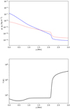Fig. 1. Vertical profiles of the equilibrium ion, 𝜚i(y), and neutral mass densities, 𝜚n(y), (top; dotted and dashed lines respectively), and the hydrostatic equilibrium temperature, T(y), taken from Avrett & Loeser (2008; bottom).

where p_0 n (p_0 i) is neutral (ion) pressure at the reference point y_ref = 50 Mm, and

$$\begin{array}{c}\hfill {\mathrm{\Lambda }}_{\mathrm{n}}=\frac{k_{\mathrm{B}}T(y)}{m_{\mathrm{H}}{\mu }_{\mathrm{n}}g},{\mathrm{\Lambda }}_{\mathrm{i}}=\frac{k_{\mathrm{B}}T(y)}{m_{\mathrm{H}}{\mu }_{\mathrm{i}}g},\end{array}$$(14)

are respectively the neutral and ion pressure scale-heights.

As a consequence of the temperature variation, the ionization degree, specified as 𝜚_i(y)/𝜚_n(y), depends on altitude in the solar atmosphere. In the photosphere, which is the layer occupying the region 0 <  y <  0.5 Mm and where the temperature is only about 5600 K, the plasma is weakly ionized with only one ion for every approximately 10³ neutrals, while in the hot solar corona (∼1 million K), which spans from the transition region located at y ≈ 2.1 Mm (see Fig. 1, bottom), the plasma is essentially fully ionized. Figure 1 (top) illustrates the vertical profiles of the mass densities of ions and neutrals. We note that the ion mass density is much lower than the neutral mass density in the photosphere and the low chromosphere. These two densities become comparable about 900km below the transition region. Higher up, the neutrals are more abundant than ions and in the low corona the mass density of the neutrals experiences a sudden fall-off with height.

In our hydrostatic equilibrium, the temperature of both ions and neutrals (Fig. 1, bottom) reaches a minimum of T = 4300 K at the top of the photosphere (500km) and increases suddenly in the transition region between the chromosphere and the low corona, which is located at y = 2.1 Mm.

3.2. Current-free magnetic field

In the equilibrium model, we adopt a current-free (∇ × B = 0) magnetic field, B = [B_x,  B_y,  B_z], which describes a solar magnetic flux-tube (Low 1985):

$$\begin{array}{c}\hfill \begin{array}{cc}& B_x(x,y)=\frac{-2Sx(y-a)}{{(x^2+{(y-a)}^2)}^2},\hfill \\ \hfill & B_y(x,y)=\frac{S(x^2-{(y-a)}^2)}{{(x^2+{(y-a)}^2)}^2}+B_{\mathrm{v}},\hfill \\ \hfill & B_z(x,y)=0,\hfill \end{array}\end{array}$$(15)

where B_v = 5 G is the magnitude of a straight vertical magnetic field component, a = −0.3 Mm is the vertical location of the singularity in the magnetic field, and S is a free parameter corresponding to the magnetic field strength. We set S so that the maximum value of |B| ≈ 82 G and is reached at the flux-tube foot point, (x = 0, y = 0) Mm. The spatial profile of the magnetic field lines and the corresponding magnetic field strength, B(x, y), are displayed in Fig. 2 (left). We note that magnitude of the magnetic field falls off from the flux-tube foot point and the magnetic field lines become essentially vertical in the corona.

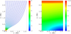Fig. 2. Spatial profiles of equilibrium magnetic field lines (left) and the Alfvén speed, cA(x, y), (right). The magnetic field strength, B(x, y), is expressed in Gauss, while cA is expressed in km s−1. Only a part of the right side of the simulation box is displayed.

The spatial profile of the Alfvén speed, $c_{\mathrm{A}}(x,y)=B/\sqrt{\mu ({\varrho }_{\mathrm{i}}+{\varrho }_{\mathrm{n}})}$, is illustrated in Fig. 2 (right). In the upper photosphere and the lower chromosphere, the Alfvén speed c_A attains values lower than 10 km s⁻¹ along the flux-tube center, given by x = 0 up to y ≈ 0.6 Mm. Higher up, as a result of the low total ion + neutral mass density, c_A rises to values above 40 km s⁻¹ until the transition region, where it experiences a sudden growth to values close to 300 km s⁻¹.

3.3. Analytically estimated wave damping

In this section we first discuss the results of analytical estimates of the damping rate of Alfvén waves in the photosphere and chromosphere.

The dispersion relation for Alfvén waves propagating in a homogeneous medium can be written as (Zaqarashvili et al. 2011; Soler et al. 2013; Ballester et al. 2018a)

$$\begin{array}{c}\hfill {\omega }^3+i(1+\chi ){\nu }_{\mathrm{ni}}{\omega }^2-k^2{c}_{\mathrm{A}}^2\omega -i{\nu }_{\mathrm{ni}}{k}^2{c}_{\mathrm{A}}^2=0,\end{array}$$(16)

where

$$\begin{array}{c}\hfill {\nu }_{\mathrm{ni}}=\frac{{\alpha }_{\mathrm{in}}}{{\varrho }_{\mathrm{n}}}\end{array}$$(17)

are respectively the ion-neutral and neutral-ion collision frequencies, χ = 𝜚_n/𝜚_i denotes ionization fraction, k is the wave number, ω the cyclic frequency, and i stands for the imaginary unit, such that i² = −1. We solve the above dispersion relation for a real value of ω = 2π/P_d, where P_d is the wave period, to find the real, k_r, and imaginary, k_i, parts of k, given as

$$\begin{array}{c}\hfill k^2=\frac{{\omega }^2}{c_{\mathrm{A}}^2}\frac{\omega +i(1+\chi ){\nu }_{\mathrm{ni}}}{\omega +i{\nu }_{\mathit{ni}}},k=k_{\mathrm{r}}+i{k}_{\mathrm{i}}.\end{array}$$(18)

The above result allows us to estimate the wavelength, λ_r = 2π/k_r, and the damping length, λ_i = 1/k_i, of the excited Alfvén waves.

Figure 3 illustrates the analytically obtained values of λ_i for both photospheric (solid line) and chromospheric (dashed line) conditions. The photosphere is dominated by neutrals, and therefore the specified values of ion and neutral mass densities are respectively 𝜚_i = 4.7 × 10⁻¹⁰ g cm⁻³ and 𝜚_n = 2 × 10⁻⁷ g cm⁻³. The corresponding values in the chromosphere are 𝜚_i = 1.7 × 10⁻¹² g cm⁻³ and 𝜚_n = 2.1 × 10⁻¹² g cm⁻³, and as a result χ in the photosphere and chromosphere differs by three orders of magnitude. A strongly coupled photospheric plasma is characterized by a friction coefficient α_in seven orders of magnitude larger there than in the chromosphere (6.5 × 10⁻³ vs. 2.6 × 10⁻¹⁰). The magnetic flux tube, given by Eq. (15), results in c_A = 3.1 km s⁻¹ at the photospheric level and c_A = 30 km s⁻¹ in the chromosphere. We conclude that Alfvén waves of P_d <  0.1 s are strongly damped in the photosphere on a distance spanning from about a few meters up to 15 km. The situation is different in the chromosphere, however. Although wave periods shorter than P_d ≈ 0.1 s are still strongly damped there, the damping length is almost constant at a value of λ_i ≈ 2.3 km. Waves with longer wave periods are more weakly damped and propagate up to the transition region and higher up into the corona. We note that for P_d >  1, the damping lengths in the photosphere and chromosphere are identical. This scenario may differ depending on the model. Cranmer & van Ballegooijen (2005) investigated the process of Alfvén wave reflection in the stratified atmosphere, concluding that Alfvén waves are reflected mostly below the transition region and this process is at its maximum at the photosphere with the reflection coefficient of 0.99825 for a period of about 40 min, whereas shorter wave periods experience weaker reflection. In our simulations, Alfvén waves are affected by reflections in the stratified atmosphere, essentially from regions of abrupt variations in Alfvén speed. However, the wave damping remains the dominant process in the attenuation of Alfvén wave amplitude.

Fig. 3. Analytically obtained damping length, λi, of Alfvén waves in the photosphere (solid line) and chromosphere (dashed line) vs. wave period Pd.

4. Numerical results

We use the JOANNA code to solve Eqs. (1)–(7). This code is based on high-order Godunov-type methods (Wójcik et al. 2018, 2019) and uses the divergence-cleaning method of Dedner et al. (2002) to control the ∇ ⋅ B = 0 constraint.

Unless otherwise stated, we extend the 2.5D simulation box from −2.56 Mm to 2.56 Mm in the x-direction and from 0 to 50 Mm in the y-direction, and cover the simulation region above the photosphere (y = 0) and below the low corona (y = 2.56 Mm) by a uniform grid of 1024 × 512 cells which leads to a uniform grid with a spatial resolution of Δx = Δy = 5 km. We chose this grid to minimize numerical diffusion which essentially does not affect Alfvén wave propagation from the lower atmospheric regions. Above the level y = 2.56 Mm we divide the simulation box into several patches of progressively larger cells along the y-direction. Such a stretched grid plays the role of a sponge as it absorbs the incoming signal and minimizes spurious reflections from the top boundary which could pollute our simulations.

We implement fixed boundary conditions at the bottom and top of the simulation box at which we set all plasma quantities to their equilibrium values. The only exception are the transverse components of the ion and neutral velocities, which in order to study Alfvén waves are specified in the form of a periodic driver acting at the bottom of the photosphere at y = 0. Specifically, we define

$$\begin{array}{cc}& V_{\mathrm{i}z}(x,y=0,t)=V_{\mathrm{n}z}(x,y=0,t)\hfill \\ \hfill & =V_{0}xexp(-\frac{x^2}{w^2})sin\left(\frac{2\pi }{P_{\mathrm{d}}}t\right),\hfill \end{array}$$(19)

where V₀ is the amplitude of the driver, w its width, and P_d the period. We allow V₀ to vary in the way that the effective amplitude of the driver lies within the range of 0.01 km s⁻¹ and 1 km s⁻¹. These amplitudes are in the observational context of a power-law spectrum for the quiet Sun. EUV intensity and Doppler shift variations (Mathioudakis et al. 2013) for low-energy and short-wave periods, could mimic the action of p-modes. However, the latter exhibit much lower amplitudes (≈10⁻⁴ km s⁻¹) than those used in our work. Instead, our periodic driver is associated with the solar granulation with horizontal velocities of a fraction of 1 km s⁻¹. Additionally, we impose open boundary conditions for outflowing signals at the side boundaries, x = ±2.56 Mm.

4.1. Numerically estimated Alfvén waves damping

In this section we discuss the numerically obtained results about the propagation and damping rate of Alfvén waves in this two-fluid setup.

First, we run the 1D simulations of damping of Alfvén waves in the photosphere. We set our numerical experiment with a uniform, high-spatial-resolution grid of Δx = Δy = 50 m, and uniform vertical magnetic field with its magnitude B = 50 Gauss. Such a fine grid allows us to significantly reduce numerical damping of the waves in our system. We specify the driver at the bottom boundary by Eq. (19), and run these simulations for a wide range of amplitudes, starting with the linear case of 1 m s⁻¹ up to a strongly nonlinear case with an amplitude of 40 km s⁻¹. The obtained results reveal strong wave damping that occurs already in the photosphere. In particular, Fig. 4 illustrates the vertical profiles of the z-component of the ion velocity, V_i z(y), at t = 50 s, t = 200 s, and t = 500 s in the case of the driving period P_d = 30 s and the amplitude V₀ = 40 km s⁻¹, that is, the strongly nonlinear case. The Alfvén waves are completely attenuated before they can reach the height y = 0.15 Mm. We note that this attenuation length does not correspond to the collisional damping length resulting from Eq. (16). For P_d <  1 s, wave damping is due to ion–neutral collisions, while for P_d >  1 s, the Alfvén waves are affected by the cut-off period and the turning point, the latter being very low for long-period waves (Wójcik et al. 2017). Further investigation of nonlinear Alfvén waves will be the subject of future studies.

Fig. 4. Vertical profiles of the z-component of the ion velocity, Vi z(y), at t = 50 s (solid line), t = 200 s (dashed line), and t = 500 s (dotted line) in the case of the driving period Pd = 30 s and the amplitude V0 = 40 km s−1, for the uniform vertical magnetic field of By = 50 G.

Figure 5 shows the spatial profile of the z-component of the ion velocity, V_i z(x, y, t), obtained by means of numerical simulations for the magnetic field given by Eq. (15) at six instants in time, namely at t = 180 s, t = 250 s, t = 500 s, t = 750 s, t = 1250 s, and t = 2300 s (from top-left to bottom-right) for P_d = 30 s and V₀ = 10 m s⁻¹. We clearly see that the driver excites transversal plasma oscillations propagating along the expanding solar magnetic flux tube. These waves are strongly damped in the upper photosphere (0 <  y <  0.3 Mm). Higher up, in the chromosphere, the amplitude exponential growth with the distance equal to the pressure-scale height (e.g., Kuźma & Murawski 2018) becomes dominant. At these altitudes the coupling between ions and neutrals is already weaker, and therefore neutrals do not follow exactly the same evolution as the ions (not shown).

Fig. 5. Spatial profiles of the z-component of the ion velocity, Vi z(x, y), at t = 180 s, t = 250 s, t = 500 s, t = 750 s, t = 1250 s, and t = 2300 s (from top-left to bottom-right) expressed in units of 1 m s−1. The case of the driving period Pd = 30 s and the amplitude V0 = 10 m s−1.

The above-mentioned damping of Alfvén waves results from the fact that the transversal neutral velocity component, V_n z, is strongly damped (e.g., Zaqarashvili et al. 2011). This results in a significant difference between the transversal components of the ion and neutral velocities, |V_i z − V_n z|. Figure 6 (top-left) illustrates the heating rate resulting from ion-neutral collisions, Q_i, which following Eq. (11) coincides with the ion–neutral drift, |V_i − V_n| (not shown). We infer that due to a large value of this drift, a fraction of the energy initially carried by Alfvén waves is thermalized in the bottom layer of the photosphere. Indeed, Fig. 6 (top-right) reveals a growth of the plasma temperature close to the bottom boundary up to δT_i ≈ 200 K over a timescale of 250 s. We note that acoustic (Kuźma et al. 2019) and fast magneto-acoustic waves (Popescu Braileanu et al. 2019) behave differently from Alfvén waves, as they contribute to plasma heating in the chromosphere, whereas Alfvén waves directly thermalize their energy in the low photosphere. A first attempt to understand how the heating and cooling processes modify the properties of MHD waves in a fully ionized medium in the case of solar prominence was made by Ballester et al. (2016). These studies were later extended to the partially ionized case (Ballester et al. 2018b), and the authors revealed that wave periods and damping times of MHD waves become time dependent when considering the heating and cooling processes. Moreover, in the case of Alfvén waves, the cut-off wave periods also become time dependent and the attenuation rate is completely different. Moreover, this temperature gradient in the solar atmosphere would be subject to thermal conduction, which is not considered in our model. Indeed, Soler et al. (2019) suggested, that thermal conduction and radiative loses could play an influential role in Alfvén-wave propagation and damping in the solar atmosphere and that such simulations should be performed. We are considering this as a topic for a future study.

Fig. 6. Time-distance plots of the heating rate resulting from ion–neutral collisions, Qi(y, t) (top-left), perturbed ion temperature, δTi(y, t) (top-right), the squared transversal component of the magnetic field, $B_z^2$ (bottom-left), and the vertical component of ion velocity, Vi y (bottom-right) evaluated at x = 0.1 Mm for the driving period Pd = 30 s and the amplitude V0 = 0.4 km s−1.

However, Alfvén waves drive magneto-acoustic waves through a gradient in magnetic pressure. This is illustrated in Fig. 6 (bottom-left) and means that Alfvén waves act as a driver generating magneto-acoustic waves. These waves are associated with V_i y and they propagate upwards into higher layers of the chromosphere (bottom-right). Hence, Alfvén waves, which are damped in the photosphere, lead to both a local temperature increase at the bottom of the photosphere and the excitation of magneto-acoustic waves.

The amplitude of the magneto-acoustic waves that are driven by Alfvén waves) is proportional to the amplitude of the driver. Figure 7 illustrates spatial profiles of ${\overline{V}}_{\mathrm{i}}(x,y)=\sqrt{V_{\mathrm{i}x}^2+V_{\mathrm{i}y}^2}$ for the driving period P_d = 30 s and the amplitude V₀ = 0.4 km s⁻¹ at four instants in time, namely at t = 1000 s, t = 1250 s, t = 1500 s, and t = 2000 s (from top-left to bottom-right). From this figure, we infer that Alfvén-wave-driven magneto-acoustic waves have higher amplitudes than the amplitude of the driver exceeding 1 km s⁻¹. We note that, as in our simulations where we implemented the realistic mass density profile, waves can experience amplitude growth with height without providing any external energy; this growth results from momentum conservation, and the carried energy does not increase with y. We also note that the regions with the largest values of ${\overline{V}}_{\mathrm{i}}$ are located in the photosphere (0.1 Mm < y <  0.3 Mm) and in the middle to upper chromosphere (y >  1.25 Mm). In the photosphere, the plasma experiences mostly a drift in horizontal direction, while chromospheric plasma moves essentially along the vertical magnetic field lines. Below, we show that these are the regions where the plasma is heated the most.

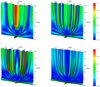Fig. 7. Spatial profiles of ${\overline{V}}_{\mathrm{i}}(x,y)=\sqrt{V_{\mathrm{i}x}^2+V_{\mathrm{i}y}^2}$, corresponding to magneto-acoustic waves at t = 1000 s, t = 1250 s, t = 1500 s, and t = 2000 s (from top-left to bottom-right) expressed in units of 1 km s−1. Here, the driving period Pd = 30 s and the amplitude V0 = 0.4 km s−1.

Figure 8 (top row) shows time–distance plots of ion magneto-acoustic waves characterized by perturbations in V_i x and V_i y. We see that V_i x dominates in the upper photosphere (top-left), where the magnetic field lines are strongly curved and almost become horizontal, while V_i y prevails in chromospheric regions that are permeated by vertical magnetic field (top-right). The energy of these waves is deposited in the form of thermal energy heating the plasma, and the energy is released during ion–neutral collisions; see also Kuźma et al. (2019) who showed that two-fluid acoustic waves with their wave periods of 30 − 120 s effectively heat chromospheric plasma. Indeed, Fig. 8 (bottom-left) displays time–distance plots of $log|{\overline{V}}_{\mathrm{i}}-{\overline{V}}_{\mathrm{n}}|$. The phase-shift between ion and neutral waves in the upper photosphere and the chromosphere results in a significant difference between ${\overline{V}}_{\mathrm{i}}$ and ${\overline{V}}_{\mathrm{n}}$. From Eq. (11) we infer that this velocity difference results in nonzero values of Q_i and thus in a growth of δT_i in time. Figure 8 (bottom-right) displays a time–distance plot of the perturbed ion temperature averaged over the whole horizontal distance (d = 5.12 Mm), $⟨\delta T_{\mathrm{i}}(y)⟩={\int }_{-d/2}^{d/2}{T}_{\mathrm{i}}(x,y)\mathrm{d}x/d$. Analyzing ⟨δT_i(y)⟩ we find that plasma in the lower photosphere 0 <  y <  0.3 Mm and in the chromosphere 1 Mm < y <  1.5 Mm is significantly heated. This heating coincides with V_i x in the photosphere and V_i y in the chromosphere. We note that the excited magneto-acoustic waves have wave periods close to 180 s. This periodicity may result from local a cut-off period and all generated wave periods will tend to this value; see also Wójcik et al. (2017) for the discussion on Alfvén wave cut-offs.

Fig. 8. Time–distance plots of Vi x(x = 0.1 Mm,y, t) (top-left) and Vi y(x = 0.1 Mm,y, t) (top-right), $log|{\overline{V}}_{\mathrm{i}}-{\overline{V}}_{\mathrm{n}}|(x=0.1$ Mm, y, t) (bottom-left) expressed in units of 1 km s−1, and ⟨δTi(y, t)⟩ expressed in Kelvin (bottom-right) for the driving period Pd = 30 s and the amplitude V0 = 0.4 km s−1.

4.2. Heating by two-fluid Alfvén waves

In this section we present an estimation of the energy and mass transport by Alfvén waves. The transversal ion mass density and energy fluxes transported by Alfvén waves can be estimated as F_𝜚 i(x, y, t) = 𝜚_iV_i z and $F_{\text{E}}(x,y,t)\approx {\varrho }_{\text{i}}{c}_{\text{A}}{V}_{\text{i} z}^2$ (Mathioudakis et al. 2013). The vertical profile of horizontally and temporarily averaged mass and energy fluxes are shown in Fig. 9. Despite the high values of both mass and energy fluxes carried by Alfvén waves in the photosphere, the signal in V_i z is attenuated very quickly (solid line). We clearly see that V_i z (corresponding to Alfvén waves) is partially transferred into magneto-acoustic waves (denoted by both the dotted line for V_i x and by the dashed line representing V_i y). Moreover, we conclude that the plasma escaping into the corona above the transition region carries a significant amount of mass density and energy, possibly contributing to overall plasma outflows and solar wind (Wójcik et al. 2019). We note that the obtained values of mass and energy fluxes lay within the range of theoretical findings for energy losses in the upper chromosphere estimated by Withbroe & Noyes (1977). However, this statement does not mean that Alfvén waves effectively contribute to plasma heating. To correctly estimate the impact of propagating waves in terms of plasma heating, we have to look at profiles of ⟨δT_i(y)⟩.

Fig. 9. Vertical profiles of horizontally and temporarily averaged ion mass, ⟨F𝜚i(y)⟩, and energy, ⟨FE(y)⟩, fluxes for the driving period Pd = 30 s and the amplitude V0 = 0.4 km s−1. Solid, dotted, and dashed lines correspond to z-, x-, and y-components, respectively.

Figure 10 illustrates the heating rate resulting from ion–neutral collisions, that is, the first term in the expression for Q_i (see Eq. (11)), versus height, y. This term depends on the ion-neutral drift, $|{\overline{V}}_{\mathrm{i}}-{\overline{V}}_{\mathrm{n}}|$. The five displayed lines correspond to ion–neutral drift values of 0.01 km s⁻¹, 0.1 km s⁻¹, 1 km s⁻¹, 10 km s⁻¹, and 100 km s⁻¹ (from bottom to top), respectively. We infer that in order to effectively heat plasma, the difference between ${\overline{V}}_{\mathrm{i}}$ and ${\overline{V}}_{\mathrm{i}}$ has to be higher than 1 km s⁻¹ or, alternatively, the driver has to work continuously for a very long time. The former requirement is met for steep wavefronts only. Thus, Alfvén waves with amplitudes below 1 km s⁻¹ are very unlikely to heat the photosphere and chromosphere, as they do not steepen (enough) with height, while waves with amplitudes V₀ = 1 km s⁻¹ (and larger) can potentially heat the chromosphere.

Fig. 10. Heating rate vs. y. The lines correspond to ion neutral drift, $|{\overline{V}}_{\mathrm{i}}-{\overline{V}}_{\mathrm{n}}|$, of 0.01 km s−1, 0.1 km s−1, 1 km s−1, 10 km s−1, and 100 km s−1 (from bottom to top).

Figure 11 shows the maximum of the horizontally and temporarily averaged relative ion perturbed temperature, ⟨δT_i⟩(y)/T₀(y), versus the driving amplitude V₀ of Eq. (19) as measured at the top of the photosphere, that is, at y = 0.5 Mm (blue dots) and in the chromosphere at y = 1.25 Mm (red squares). Here T₀(y) is the equilibrium temperature (Avrett & Loeser 2008). Intuitively, higher values of V₀ are supposed to correspond to higher values of ion–neutral drift $|{\overline{V}}_{\mathrm{i}}-{\overline{V}}_{\mathrm{n}}|$ and as a result lead to higher Q_i. Following this pattern, we expect ⟨δT_i⟩/T₀ to grow in the chromosphere with V₀. Indeed, Fig. 11 reveals a growth of ⟨δT_i⟩/T₀ with increasing V₀. Moreover, we find that Alfvén waves with amplitudes lower than 0.45 km s⁻¹ excite magneto-acoustic waves that mostly heat the upper photosphere and the chromosphere. This additional heating is only up to ∼5% of the original photospheric temperature. Alfvén waves of higher amplitudes, namely between 0.5 and 0.7 km ⁻¹, excite magneto-acoustic waves that can penetrate higher layers of the atmosphere and effectively heat the chromosphere up to about twice its initial temperature. Further increase of the driver amplitude, closer to 1 km s⁻¹, leads to plasma heating above ten times its initial temperature. From Fig. 8 (bottom-right) we infer that, although the photosphere is heated almost immediately, the chromospheric plasma requires the driver to work continuously for several thousand seconds in order to be heated. This time results from the time needed for Alfvén waves to propagate, to drive magneto-acoustic waves, and for the latter to travel through the chromosphere and reflect from the transition region. We note that after this time the solar granulation in the photosphere is also developed, which can excite magneto-acoustic waves (Wójcik et al. 2019).

Fig. 11. Maximum of horizontally and temporarily averaged relative ion perturbed temperature, ⟨δTi⟩/T0, vs. the driving amplitude V0 for the driving period Pd = 30 s, collected at y = 0.5 Mm (blue dots) and y = 1.25 Mm (red squares).

Figure 12 illustrates the dependence of the maximum of the horizontally and temporarily averaged relative ion perturbed temperature, ⟨δT_i⟩/T₀ on the driving period, P_d. We infer that the plasma heating rate significantly rises for short-period Alfvén waves, while for wave periods longer than P_d = 80 s this heating remains essentially constant. The decrease of the heating for longer wave periods is most notably seen in the chromosphere.

Fig. 12. Maximum of horizontally and temporarily averaged relative ion perturbed temperature, ⟨δTi⟩/T0, vs. the driving period Pd for the driving amplitude V0 = 0.5 km s−1, collected at y = 0.5 Mm (blue dots) and y = 1.25 Mm (red squares).

5. Conclusions

We devoted this paper to the study of solar atmospheric heating by Alfvén waves in the framework of a two-fluid plasma model consisting of ions + electrons and neutrals, where ions are described by the MHD equations and neutrals are governed by the HD equations. These two distinct species of plasma interact with each other by means of collisions modeled by ion–neutral drag forces in the momentum equations.

In our model, Alfvén waves are driven by a monochromatic driver acting at the bottom of the photosphere. We find that due to ion–neutral collisions, Alfvén waves are strongly damped in the photosphere. For small amplitudes of the driver, mainly below V₀ = 0.1 km s⁻¹, these waves cannot effectively heat the solar atmospheric plasma. Although the obtained values of the energy flux of propagating Alfvén waves lay within the range of the theoretical findings for energy losses in the upper photosphere and chromosphere (Withbroe & Noyes 1977), these low-amplitude waves heat the chromospheric plasma increasing its temperature by only up to 25 K on a timescale of a few minutes. Alfvén waves differ from two-fluid acoustic waves which can thermalize their energy in the chromosphere leaving the photospheric plasma essentially intact (Kuźma et al. 2019).

However, Alfvén waves with amplitudes higher than 0.1 km s⁻¹, which can potentially be associated with the solar granulation revealing horizontal velocities being a fraction of 1 km s⁻¹, drive magneto-acoustic waves via the ponderomotive force, and these magneto-acoustic waves can have amplitudes higher than 1 km s⁻¹. Our work confirms the findings of Kuźma et al. (2019) who showed that two-fluid acoustic waves heat chromospheric plasma. We find that magneto-acoustic waves driven by nonlinear Alfvén waves can effectively heat both the photosphere and the chromosphere. However, we note that although the photospheric plasma is heated almost immediately, it requires the photospheric driver to act for a sufficiently long time (t >  4000 s) for the chromospheric plasma to be heated in this way.

Further studies are required to determine the possibility of sustaining a quasi-equilibrium solar atmosphere heated solely by Alfvén and magneto-acoustic waves, employing 3D simulations and more realistic conditions, including for example radiative losses, thermal conduction, and nonlocal thermal equilibrium in the chromosphere and resistivity terms.

Acknowledgments

This work was done within the framework of the projects from the National Science Centre (NCN) Grant nos. 017/25/B/ST9/00506 and 2017/27/N/ST9/01798. D.Y. was supported by the National Natural Science Foundation of China (NSFC, 11803005, 11911530690), the Shenzhen Technology Project (JCYJ20180306172239618) and Shenzhen Science and Technology program (Group No. KQTD20180410161218820). The JOANNA code was developed by Darek Wójcik. Numerical simulations were performed on the LUNAR cluster at Institute of Mathematics of University of M. Curie-Skłodowska, Lublin, Poland.

References

All Figures

	Fig. 1. Vertical profiles of the equilibrium ion, 𝜚i(y), and neutral mass densities, 𝜚n(y), (top; dotted and dashed lines respectively), and the hydrostatic equilibrium temperature, T(y), taken from Avrett & Loeser (2008; bottom).
In the text

	Fig. 2. Spatial profiles of equilibrium magnetic field lines (left) and the Alfvén speed, cA(x, y), (right). The magnetic field strength, B(x, y), is expressed in Gauss, while cA is expressed in km s−1. Only a part of the right side of the simulation box is displayed.
In the text

	Fig. 3. Analytically obtained damping length, λi, of Alfvén waves in the photosphere (solid line) and chromosphere (dashed line) vs. wave period Pd.
In the text

	Fig. 4. Vertical profiles of the z-component of the ion velocity, Vi z(y), at t = 50 s (solid line), t = 200 s (dashed line), and t = 500 s (dotted line) in the case of the driving period Pd = 30 s and the amplitude V0 = 40 km s−1, for the uniform vertical magnetic field of By = 50 G.
In the text

	Fig. 5. Spatial profiles of the z-component of the ion velocity, Vi z(x, y), at t = 180 s, t = 250 s, t = 500 s, t = 750 s, t = 1250 s, and t = 2300 s (from top-left to bottom-right) expressed in units of 1 m s−1. The case of the driving period Pd = 30 s and the amplitude V0 = 10 m s−1.
In the text

	Fig. 6. Time-distance plots of the heating rate resulting from ion–neutral collisions, Qi(y, t) (top-left), perturbed ion temperature, δTi(y, t) (top-right), the squared transversal component of the magnetic field, $B_z^2$ (bottom-left), and the vertical component of ion velocity, Vi y (bottom-right) evaluated at x = 0.1 Mm for the driving period Pd = 30 s and the amplitude V0 = 0.4 km s−1.
In the text

	Fig. 7. Spatial profiles of ${\overline{V}}_{\mathrm{i}}(x,y)=\sqrt{V_{\mathrm{i}x}^2+V_{\mathrm{i}y}^2}$, corresponding to magneto-acoustic waves at t = 1000 s, t = 1250 s, t = 1500 s, and t = 2000 s (from top-left to bottom-right) expressed in units of 1 km s−1. Here, the driving period Pd = 30 s and the amplitude V0 = 0.4 km s−1.
In the text

	Fig. 8. Time–distance plots of Vi x(x = 0.1 Mm,y, t) (top-left) and Vi y(x = 0.1 Mm,y, t) (top-right), $log|{\overline{V}}_{\mathrm{i}}-{\overline{V}}_{\mathrm{n}}|(x=0.1$ Mm, y, t) (bottom-left) expressed in units of 1 km s−1, and ⟨δTi(y, t)⟩ expressed in Kelvin (bottom-right) for the driving period Pd = 30 s and the amplitude V0 = 0.4 km s−1.
In the text

	Fig. 9. Vertical profiles of horizontally and temporarily averaged ion mass, ⟨F𝜚i(y)⟩, and energy, ⟨FE(y)⟩, fluxes for the driving period Pd = 30 s and the amplitude V0 = 0.4 km s−1. Solid, dotted, and dashed lines correspond to z-, x-, and y-components, respectively.
In the text

	Fig. 10. Heating rate vs. y. The lines correspond to ion neutral drift, $|{\overline{V}}_{\mathrm{i}}-{\overline{V}}_{\mathrm{n}}|$, of 0.01 km s−1, 0.1 km s−1, 1 km s−1, 10 km s−1, and 100 km s−1 (from bottom to top).
In the text

	Fig. 11. Maximum of horizontally and temporarily averaged relative ion perturbed temperature, ⟨δTi⟩/T0, vs. the driving amplitude V0 for the driving period Pd = 30 s, collected at y = 0.5 Mm (blue dots) and y = 1.25 Mm (red squares).
In the text

	Fig. 12. Maximum of horizontally and temporarily averaged relative ion perturbed temperature, ⟨δTi⟩/T0, vs. the driving period Pd for the driving amplitude V0 = 0.5 km s−1, collected at y = 0.5 Mm (blue dots) and y = 1.25 Mm (red squares).
In the text

References

- Alfvén, H. 1942, Nature, 150, 405 [NASA ADS] [CrossRef] [Google Scholar]
- Avrett, E., & Loeser, R. 2008, ApJS, 175, 229 [NASA ADS] [CrossRef] [Google Scholar]
- Ballester, J. L., Carbonell, M., Soler, R., & Terradas, J. 2016, A&A, 591, A109 [NASA ADS] [CrossRef] [EDP Sciences] [Google Scholar]
- Ballester, J. L., Alexeev, I., Collados, M., et al. 2018a, Space Sci. Rev., 214, 58 [NASA ADS] [CrossRef] [Google Scholar]
- Ballester, J. L., Carbonell, M., Soler, R., & Terradas, J. 2018b, A&A, 609, A6 [NASA ADS] [CrossRef] [EDP Sciences] [Google Scholar]
- Belcher, J. W., & Davis, L. 1971, J. Geophys. Res., 76, 3534 [NASA ADS] [CrossRef] [Google Scholar]
- Bierman, L. 1946, Naturwissenschaften, 33, 118 [NASA ADS] [CrossRef] [Google Scholar]
- Chmyrev, V. M., Bilichenko, S. V., Pokhotelov, O. A., et al. 1988, Phys. Scr., 38, 841 [CrossRef] [Google Scholar]
- Cranmer, S. R., & van Ballegooijen, A. A. 2005, ApJS, 156, 265 [NASA ADS] [CrossRef] [Google Scholar]
- Dedner, A., Kemm, F., Kröner, D., et al. 2002, J. Comput. Phys., 175, 645 [Google Scholar]
- Doorsselaere, T. V., Nakariakov, V. M., & Verwichte, E. 2008, ApJ, 676, L73 [NASA ADS] [CrossRef] [Google Scholar]
- Goodman, M. L. 2011, ApJ, 735, 45 [NASA ADS] [CrossRef] [Google Scholar]
- Khomenko, E. 2017, Plasma Phys. Controlled Fusion, 59, 014038 [NASA ADS] [CrossRef] [Google Scholar]
- Kulsrud, R., & Pearce, W. P. 1969, ApJ, 156, 445 [NASA ADS] [CrossRef] [Google Scholar]
- Kuźma, B., & Murawski, K. 2018, ApJ, 866, 50 [CrossRef] [Google Scholar]
- Kuźma, B., Wójcik, D., & Murawski, K. 2019, ApJ, 878, 81 [NASA ADS] [CrossRef] [Google Scholar]
- Low, B. C. 1985, ApJ, 293, 31 [NASA ADS] [CrossRef] [Google Scholar]
- Lundquist, S. 1949, Phys. Rev., 76, 1805 [CrossRef] [Google Scholar]
- Martínez-Gómez, D., Soler, R., & Terradas, J. 2018, ApJ, 856, 16 [NASA ADS] [CrossRef] [Google Scholar]
- Martínez-Sykora, J., Pontieu, B. D., & Hansteen, V. 2012, ApJ, 753, 161 [NASA ADS] [CrossRef] [Google Scholar]
- Mathioudakis, M., Jess, D. B., & Erdélyi, R. 2013, Space Sci. Rev., 175, 1 [NASA ADS] [CrossRef] [Google Scholar]
- Murawski, K., & Musielak, Z. E. 2010, A&A, 518, A37 [NASA ADS] [CrossRef] [EDP Sciences] [Google Scholar]
- Narain, U., & Ulmschneider, P. 1996, Space Sci. Rev., 75, 453 [NASA ADS] [CrossRef] [Google Scholar]
- Oliver, R., Soler, R., Terradas, J., & Zaqarashvili, T. V. 2016, ApJ, 818, 128 [NASA ADS] [CrossRef] [Google Scholar]
- Piddington, J. H. 1956, MNRAS, 116, 314 [NASA ADS] [CrossRef] [Google Scholar]
- Popescu Braileanu, B., Lukin, V. S., Khomenko, E., & de Vicente, Á. 2019, A&A, 627, A25 [NASA ADS] [CrossRef] [EDP Sciences] [Google Scholar]
- Schwarzschild, M. 1948, ApJ, 107, 1 [NASA ADS] [CrossRef] [Google Scholar]
- Soler, R., Carbonell, M., & Ballester, J. L. 2013, ApJS, 209, 16 [NASA ADS] [CrossRef] [Google Scholar]
- Soler, R., Ballester, J. L., & Zaqarashvili, T. V. 2014, A&A, 573, A79 [Google Scholar]
- Soler, R., Terradas, J., Oliver, R., & Ballester, J. L. 2019, ApJ, 871, 3 [NASA ADS] [CrossRef] [Google Scholar]
- Song, P., & Vasyliūnas, V. M. 2011, J. Geophys. Res., 116, A09104 [Google Scholar]
- Srivastava, A. K., Shetye, J., Murawski, K., et al. 2017, Sci. Rep., 7, 43147 [NASA ADS] [CrossRef] [Google Scholar]
- Tomczyk, S., McIntosh, S. W., Keil, S. L., et al. 2007, Science, 317, 1192 [NASA ADS] [CrossRef] [PubMed] [Google Scholar]
- Vögler, A., Shelyag, S., Schüssler, M., et al. 2005, A&A, 429, 335 [NASA ADS] [CrossRef] [EDP Sciences] [Google Scholar]
- Vranjes, J., & Krstic, P. S. 2013, A&A, 554, A22 [NASA ADS] [CrossRef] [EDP Sciences] [Google Scholar]
- Vranjes, J., & Poedts, S. 2009, MNRAS, 400, 2147 [NASA ADS] [CrossRef] [Google Scholar]
- Vranjes, J., & Poedts, S. 2010, ApJ, 719, 1335 [NASA ADS] [CrossRef] [Google Scholar]
- Withbroe, G. L., & Noyes, R. W. 1977, ARA&A, 15, 363 [NASA ADS] [CrossRef] [Google Scholar]
- Wójcik, D., Murawski, K., Musielak, Z. E., Konkol, P., & Mignone, A. 2017, Sol. Phys., 292, 31 [CrossRef] [Google Scholar]
- Wójcik, D., Murawski, K., & Musielak, Z. E. 2018, MNRAS, 481, 262 [NASA ADS] [CrossRef] [Google Scholar]
- Wójcik, D., Kuźma, B., Murawski, K., & Srivastava, A. K. 2019, ApJ, 884, 127 [CrossRef] [Google Scholar]
- Zaqarashvili, T. V., Khodachenko, M. L., & Rucker, H. O. 2011, A&A, 529, A82 [NASA ADS] [CrossRef] [EDP Sciences] [Google Scholar]
- Zaqarashvili, T. V., Khodachenko, M. L., & Soler, R. 2013, A&A, 549, A113 [NASA ADS] [CrossRef] [EDP Sciences] [Google Scholar]