| Issue |
A&A
Volume 639, July 2020
|
|
|---|---|---|
| Article Number | A83 | |
| Number of page(s) | 19 | |
| Section | Planets and planetary systems | |
| DOI | https://doi.org/10.1051/0004-6361/201937096 | |
| Published online | 13 July 2020 | |
Global photometric properties of (162173) Ryugu
1
Instituto de Astrofísica de Canarias (IAC), University of La Laguna,
La Laguna,
Tenerife, Spain
e-mail: This email address is being protected from spambots. You need JavaScript enabled to view it.
2
Department of Astrophysics, University of La Laguna,
La Laguna,
Tenerife, Spain
3
Department of Earth and Planetary Science, The University of Tokyo,
Bunkyo,
Tokyo, Japan
4
Planetary Science Institute (PSI),
Tucson,
AZ, USA
5
Deutsches Zentrum für Luft- und Raumfahrt (DLR),
Berlin, Germany
6
Institute of Space and Astronomical Science (ISAS), Japan Aerospace Exploration Agency (JAXA),
Sagamihara,
Kanagawa, Japan
7
Kochi University,
Kochi,
Kochi, Japan
8
Okayama Observatory, Kyoto University,
Asakuchi,
Okayama, Japan
9
Seoul National University,
Gwanak,
Seoul, Korea
10
Brown University,
Providence,
RI, USA
11
The University Museum, The University of Tokyo,
Bunkyo,
Tokyo, Japan
12
Planetary Exploration Research Center (PERC), Chiba Institute of Technology,
Narashino,
Chiba, Japan
13
Rikkyo University,
Toshima,
Tokyo, Japan
14
National Institute of Advanced Industrial Science and Technology (AIST),
Koto,
Tokyo, Japan
15
Meiji University,
Kawasaki,
Kanagawa, Japan
16
Department of Complexity Science and Engineering, The University of Tokyo,
Kashiwa,
Chiba, Japan
17
The University of Aizu,
Aizu-Wakamatsu,
Fukushima, Japan
18
Kobe University,
Kobe,
Hyogo, Japan
19
National Astronomical Observatory of Japan (NAOJ),
Mitaka,
Tokyo, Japan
Received:
11
November
2019
Accepted:
22
May
2020
Abstract
Context. The Hayabusa2 spacecraft launched by Japan Aerospace Exploration Agency has been conducting observations of the asteroid (162173) Ryugu since June 2018. The Telescopic Optical Navigation Camera (ONC-T) onboard Hayabusa2 has obtained thousands of images under a variety of illumination and viewing conditions.
Aims. Our objective is to examine and validate the camera calibration, derive a photometric correction for creating global albedo maps, and to interpret the photometric modeling results to characterize the surface of Ryugu.
Methods. We observed (162173) Ryugu with the Gemini-South telescope, and combined these measurements with other published ground-based observations of the asteroid. The ground-based observations were compared with the data obtained by ONC-T in order to validate the radiometric calibration mutually. We used a combination of the Hapke disk-integrated and disk-resolved model equations to simultaneously analyze the combined ground- and spacecraft-based data.
Results. The average spectrum of Ryugu was classified as Cb-type following the SMASSII taxonomy and C/F-type following the Tholen taxonomy based on spacecraft observations. We derived Hapke model parameters for all seven color filters, which allowed us to photometrically correct images to within an error of <10% for ~80% of the image pixels used in the modeling effort. Using this model, we derived a geometric albedo of 4.0 ± 0.5% (v band) for Ryugu. The average reflectance factor at the standard illumination condition was 1.87 ± 0.14% in the v band. Moreover we measured a phase reddening of (2.0 ± 0.7) × 10−3 μm−1 deg−1 for Ryugu, similar to that observed for the asteroid (101955) Bennu.
Conclusions. The global color map showed that the general trend was for darker regions to also be redder regions, however there were some distinct exceptions to this trend. For example, Otohime Saxum was bright and red while Kibidango crater was dark and blue. The darkness and flatness of Ryugu’s reflectance might be caused by a high abundance of organic materials.
Key words: techniques: photometric / minor planets, asteroids: individual: Ryugu / space vehicles / methods: observational
© ESO 2020
1 Introduction
The Japanese spacecraft Hayabusa2 arrived and conducted its rendezvous with the near-Earth asteroid (162173) Ryugu between June 2018 and November 2019. Hayabusa2 started its approach observations in early June and began acquiring global, disk-resolved images from its home position (an altitude of ~20 km) from July to September, 2018, using the Optical Navigation Camera (ONC, Sugita et al. 2019). The ONC is composed of three cameras, one telescopic camera, ONC-T, and two wide-angle cameras, ONC-W1 and -W2. ONC-T is equipped with seven color bandpass filters; ul: 0.40 μm, b: 0.48 μm, v: 0.55 μm, Na: 0.59 μm, w: 0.70 μm, x: 0.86 μm, and p: 0.95 μm (Kameda et al. 2017; Suzuki et al. 2018; Tatsumi et al. 2019a). ONC-T was designed to measure and map the spectrophotometric properties of the surface of the target asteroid as well as the mission operation support (i.e., the optical navigation).
One of the main objectives for ONC-T is to map both organic-related and hydrated minerals on the surface of Ryugu in order to provide information for touch-down and sample site selections. The presence of organic compounds found in carbonaceous chondrites and interplanetary dust particles is known to lower the reflectance properties of materials (Hiroi et al. 2016a). Therefore, the regions with lower reflectance may indicate areas that are richer in organic compounds. In addition, phyllosilicates could be detected by the presence of an absorption in the 0.7-μm band region (e.g., Vilas & Gaffey 1989). Phyllosilicates are abundant in CM chondrites, which are the most common carbonaceous chondrites on Earth. Detection of the presence of phyllosilicates might mean that Ryugu was aqueously altered during its early history, which favors the hypothesis that Ryugu is a potential source of the water on Earth. Since Ryugu turned out to be very dark and have little variation in spectral properties over its surface (Sugita et al. 2019), careful and accurate photometric correction is needed for mapping subtle mineral compositional variations.
Photometric analysis of the images from ONC-T have been used for (1) validating the calibration of the camera, (2) providing photometricstandardization for the construction of albedo and color maps of the surface, and (3) to gain some understanding of Ryugu’s regolith properties in comparison with other asteroids, especially those visited by spacecraft. The photometric analysis presented here was conducted using the Hapke set of equations (e.g., Hapke 2012). The Hapke set of photometric model equations, derived from radiative transfer theory, have been widely applied to many planetary surfaces to describe their photometric reflectance behavior (e.g., Domingue et al. 2002, 2015; Li et al. 2004, 2013; Hasselmann et al. 2017; Tatsumi et al. 2018). This study places Ryugu in context with these other objects.
Before the arrival of Hayabusa2 at Ryugu, the photometric and spectroscopic properties of Ryugu were intensively investigated using ground-based observations. In addition, here we provide the unpublished ground-based visible spectra of Ryugu obtained with the Gemini-South 8.1m telescope in 2012. The first photometric model of Ryugu was provided by Ishiguro et al. (2014), which modeled the V -band photometric properties of Ryugu by the Hapke disk-integrated model (Hapke 1984) in wide phase angle range. The results of this modeling suggested the very dark nature of Ryugu with the geometric albedo of 0.047 ± 0.003. After arrival at Ryugu, Sugita et al. (2019) conducted photometric modeling based on the spacecraft data combined with ground-based observations. These latter authors modeled only v-band with a limited spacecraft dataset with a phase angle of 16°–20°. In this study, we compile data from ground-based observations and the imaging observations of Hayabusa2 during its approach and at a 20 km distance from Ryugu. It should be noted that we used a wider range of phase angles than Sugita et al. (2019), including close to opposition, and we modeled all seven band filters to extract the wavelength dependency on photometric properties. We analyze this combined data set to demonstrate the robustness of the camera calibration, provide insight into the regolith properties, and construct global albedo and color maps of Ryugu’s surface.
Observation conditions.
2 Spectrophotometric data sets
The analyses presented in this study consist of the examination of two sources of data: those acquired by ground-based telescopes and those extracted from the ONC-T/Hayabusa2 images. Here we discuss each data set and the processing that was applied to extract the spectrophotometric measurements needed for analysis. We compare the photometric and spectroscopic properties of the two data sets. This comparison is key to validating the calibration of ONC-T.
2.1 Visible spectral observation of (162173) Ryugu with Gemini-South telescope
We conducted a series of visible spectroscopic observations of (162173) Ryugu with the 8.1m-aperture Gemini-South telescope at Cerro Pachón in Chile using the GMOS instrument (Hook et al. 2004) on 24 and 26 June and 5 July, 2012. The observational conditions are summarized in Table 1. The apparent visible magnitude of Ryugu was between 19.13 and 19.66 during our observations (Fig. 1a). These three nights of observations covered a wide range of rotational phases (Fig. 1b). The phase angle range was relatively small, between 22.7° and 30.3°. A G2V star, HD 142801 was used as a solar analog star for calibration. This star was located close to Ryugu (airmass difference <0.1) during the observations. Observational error was estimated based on the scatter among the four exposures and is given as error bars in Fig. 2. Flat field correction and sky subtraction were conducted using standard procedures (e.g., Kuroda et al. 2014) with the GEMINI IRAF software package.
Four integrations of 900 s of exposure were conducted for each observation. The four exposures are added together to increase the signal-to-noise ratio (S/N). The resulting photon counts are large enough that shot noise is at a negligible level. All three nights of observations contain substantial noise due to fringe pattern at longer wavelengths; data for wavelengths longer than ~0.8 μm are unreliable. Therefore, data at >0.8 μm are not usedfor further analyses in this study. The observations on 5 July suffered from background star contamination leading to a higher noise level. Nevertheless, the noise level is low enough that the spectral data can be used for further analyses. The remaining two spectral data sets for <0.8 μm have a low noise level of 2σ ~ 3%.
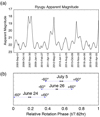 |
Fig. 1 Timing of our Ryugu observations using the Gemini-South telescope. (a) Apparent visual magnitude (AP-mag) of asteroid Ryugu provided by HORIZONS (https://ssd.jpl.nasa.gov/horizons.cgi). Our visible spectra were observed during the last observation opportunity (summer of 2012) before the launch of Hayabusa2 in December 2014. (b) Comparison of the rotational phases among our three observations. The black lines indicate the length of observations for these three nights. The blue lines indicate rotational phases that would have been observed at the respective observation times. |
2.2 Ground-based observations from previous work
The ground-based data set in this study consisted of the disk-integrated photometric phase curve observations cited in Ishiguro et al. (2014) and a set of spectral observations that were convolved with the ONC-T filter response functions to create additional photometric phase curve observations. The Ishiguro et al. (2014) data set was acquired at various wavelength filters reduced into the reflectance at Johnson-Cousins V band, which corresponds to the ONC-T v-band central wavelength. The convolved spectral observations provide additional phase curve data points at 0.55 μm, and the only phase curve data corresponding to the remaining ONC-T filter wavelengths.
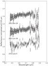 |
Fig. 2 Spectra of (162173) Ryugu obtained with the Gemini-South telescope on 24 and 26 June and 5 July, 2012. Spectra are normalized to unity at 0.55 μm and offsets between spectra are 0.2. |
2.2.1 Ishiguro et al. (2014) data set
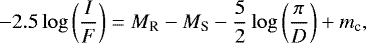
Ishiguro et al. (2014) collected phase curve observations spanning from 0.25° to 78.77° in phase angle. The observations were measured in terms of magnitude and converted to reflectance (I/F) using the relationship
 (1)
(1)
where MR is the observed magnitude of Ryugu, MS is the V -band magnitude of the Sun at 1 au (MS = −26.74, Allen 1973), and D is the apparent cross section of Ryugu (D = 6.25 × 10⁵ m2, assuming the equivalent area of a circle with a diameter of 892 m, which is the diameter determined from the shape model used in Watanabe et al. 2019), and mc = −55.87 (a constant used by Ishiguro et al. 2014 to adjust the length unit). The value for D in this study differs from that used by Ishiguro et al. (2014) because these latter authors adopted a diameter of 870 m which was determined before the rendezvous phase (Müller et al. 2011).
2.2.2 Spectral observations
Several ground-based spectral observations (Table 2) were averaged with the ONC-T filter response functions (Kameda et al. 2017) to create equivalent disk-integrated phase curve observations for each filter for wide phase angle range. The spectra used were all normalized to unity at 0.55 μm, and therefore to convert back to absolute reflectance a method was needed to calculate the reflectance at 0.55 μm for the phase angle conditions of the spectral observations. The Ishiguro et al. (2014) data set was fit with a fifth-order polynomial. This polynomial was used to calculate the disk-integrated reflectance at 0.55 μm for each of the spectral observations at their corresponding phase angle. This provided a multiplicative factor to convert the broadband spectrum from the normalized to absolute reflectance.
2.3 Hayabusa2 observations
Hayabusa2 began approach observations of Ryugu at the beginning of June 2018 at a distance of ~2600 km. On 27 June Hayabusa2 arrived at the home position, an altitude of ~20 km above Ryugu, and conducted check-out operations, such as exposure-time and stray-light checks, and flat-field validation. After arrival, a sequence of observations was conducted for scientific evaluation of candidate sites for touch-down (TD) and sample operations. Table 3 summarizes the observations from arrival until the beginning of 2019. The operations were categorised by their objectives: for example, the objective of “Box-A” was global mapping with ~2 m pix−1 at the home position; the objective of “Box-B” was observations with a variety of viewing geometries; and “Box-C” was observations with different resolutions and viewing geometries. We analyzed the photometric properties of Ryugu using data from the approach phase and at 20 km distance, that is, ~2 m pix−1, such as pre-Box-A, Box-A1, Box-B2, and Box-B3. All images contain the whole object in the field of view (FOV). In particular, we included Box-B2 operation images, where the phase angle varied between 16.0° and 40.7°, in order to measure the photometric phase curves of Ryugu in all seven bands. The aim of Box-B3 was to observe Ryugu at opposition. The observational geometry of each pixel, such as incidence, emission, and phase angles, was calculated based on the shape model SHAPE_SFM_3M_v20180804 (Watanabe et al. 2019) and SPICE kernels utilizing the NAIF SPICE toolkit (Acton 1996). This shape model has a polygon size of ~1.5 m, which is comparable to the pixel scale observed from 20 km. The disk-resolved reflectance was obtained by the radiance factor images described in the calibration flow in Tatsumi et al. (2019a). It should be noted that we used the updated flat-fields by Tatsumi et al. (2019b). The disk-integrated reflectance was obtained as in Tatsumi et al. (2018), integrating the radiance factor images including scattered light around the object. We calculated the disk-integrated reflectance using improved determinations for Ryugu’s size and dimensions. We used all images of pre-Box-A, Box-A1, Box-B2, and Box-B3 for disk-integrated analysis and only Box-B2 for disk-resolved analysis.
2.4 Data comparisons
ONC-T/Hayabusa2 disk-integrated phase curves and spectra can be compared with ground-based observations. Figure 3 shows the phase curve comparisons between the ONC-T/Hayabusa2 and ground-based observations by Ishiguro et al. (2014). The overlap indicates that the radiometric calibration for ONC-T is well within the error bars of both datasets.
Figure 4 shows the one rotational average spectra of Ryugu with different phase angles. We observed very weak phase reddening, although the spectral slope variation was smaller than the variation by rotational phase difference (error bar is 1-σ of rotational variation in Fig. 4). The phase reddening is further discussed in Sect. 5.1. The average spectrum suggests Ryugu can be classified as C-complex class due to its flat slope in visible wavelength. However, the subtype classification is more difficult because of its unique spectral feature of upturn in UV. With the definition by Bus & Binzel (2002), the UV absorption feature divides the C-complex class into C and Cb types. Ryugu is classified to Cb type, although the mean visible spectral slope of Ryugu is reminiscent of both C and Cb type. According to the taxonomy by Tholen (1984), although the visible spectral slope is closer to the mean of C type than that of F type, the feature of upturn in UV suggests that Ryugu is more similar to F type (Fig. 5). According to Tholen (1984) taxonomy, Ryugu is anintermediate type of asteroid between C and F type. Although B and F types in Tholen (1984) taxonomy cannot be distinguished in Bus & Binzel (2002), the wide coverage of the ONC-T filter down to 0.4 μm allows us to classify Ryugu as a C- or F-type but not a B-type.
Spectra from both ground- and spacecraft-based datasets normalized to unity at 0.55 μm show similarities in spectral shape (Fig. 6). Flat spectra similar to the September 2007 spectrum by Vilas (2008) and that by Moskovitz et al. (2013) were observed in our three ground-based observations (Fig. 2). Although there seems to be a hint of 0.7-μm band absorption on 5 July, the absorption is smaller than the noise level. There is no obvious 0.7-μm absorption band in our ground-based spectra. The fact that three flat spectra without clear 0.7-μm absorption were observed at different rotation phases strongly suggests that most of Ryugu’s surface may be covered by material characterized by a flat spectrum, at least in the latitude range seen from the Earth during our observation period.
We can also compare the ONC-T and ground-based observations in terms of spectral properties. To quantitatively assess those observations with a variety of conditions, we bin spectra by 0.02 μm in order to decrease the dependency on wavelength resolution brought about by the different grisms used in different observations. Noise is evaluated as the deviation inside each bin. Red points in Fig. 6 show the binned spectra and their error bars. The observations with high S/R or low airmass are consistent with ONC-T observations showing very flat spectra, while some of them have poor S/R values and they are far from ONC-T observations. Previous studies discussed variation in the 0.7-μm and UV drop-off. However, it turns out there is very little spectral variation on Ryugu, meaning that some of the ground-based observations were affected by poor signal caused especially by atmospheric and airmass conditions. For example, B01, V01, L01, and L03 show the drop-off in near-UV, which is not observed onboard due to relatively large airmass. The S/N is highly dependent on the aperture of the telescope used. We found that even high-S/N observations among the largest 8.2 m telescope, ESO-VLT, show mismatch when the airmass is large. Hence, the quality of spectra is sensitive to the airmass condition. Excluding the observations with airmass >1.1, the spectra are very flat but have a slightly positive spectral slope and are consistent with the ONC-T onboard observation. This consistency supports the robustness of the ONC-T radiometric calibrations. We note that we see the absorption towards 1 μm for the ONC-T observations, which could be indicative of mafic minerals such as olivine and pyroxene. For example, thermal metamorphosed carbonaceous chondrites exhibit a wide absorption feature around 1μm (Cloutis et al. 2012). However, according to the error in the sensitivity calibration of 3% (Tatsumi et al. 2019a), the absorption could be measurement error. Further investigations are required based on local variation of 1-μm band absorption using resolved image analyses in order to make any firm conclusions.
Ground-based spectral observations.
ONC observations between June 2018 and January 2019.
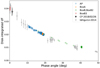 |
Fig. 3 Disk-integrated phase function for v band by ONC-T/Hayabusa2 (blue, red, green, black symbols) and by Ishiguro et al. (2014, gray symbols). |
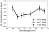 |
Fig. 4 Disk-average spectra of Ryugu with different phase angles. Error bars are 1-σ of different variation by rotational phase. |
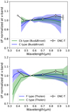 |
Fig. 5 Disk-average spectrum of Ryugu with taxonomy classification of Tholen (1984) and Bus & Binzel (2002). Hatched areas show the high and low values among those classes. Error bars were calculated based on the error in sensitivity calibration in Tatsumi et al. (2019a). |
3 Photometric modeling approach and methodology
The Hapke (1981, 1984, 1986, 2002) photometric model has been widely used by the planetary science community to analyze the nature of particulate surfaces of atmosphereless celestial bodies. The Hapke model is based on the equations of radiative transfer andits parameters can arguably be interpreted in terms of the physical properties of the surface (Hapke 2012). However, the model has been the subject of criticism for apparent correlations between supposedly independent parameters and difficulties in linking the parameters to physical surface properties (Gunderson et al. 2006; Shepard & Helfenstein 2007; Shkuratov et al. 2012). Some model parameters may represent complex combinations of particle properties, surface roughness, and packing state (Shepard & Helfenstein 2007). Recent versions of the model appear to perform better, and the debate is ongoing (Ciarniello et al. 2014; Shepard & Helfenstein 2011; Labarre et al. 2017). Regardless of whether the Hapke model accurately describes the physics of regolith scattering, the model has been widely used and Hapke’s parameters are available for many planetary objects. Our observations with ONC-T cover a wide range of illumination conditions, which allows us to tightly constrain the Hapke parameters. In addition, because the Hapke model has been intensively used for many objects, it is worth conducting a comparative study with Hapke’s parameters.
For each ONC-T filter, we collected two types of photometric measurements: (1) the disk-integrated phase curves using both ground- andspacecraft-based observations, and (2) disk-resolved photometric measurements extracted from the Box-B2 image sets. Here we describe the models used to analyze each data set, and the approach used for deriving a description of the global photometricbehavior of Ryugu’s surface.
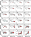 |
Fig. 6 Comparison between the 24 ground-based spectra (Binzel et al. 2001; Vilas 2008, 2012; Moskovitz et al. 2013; Lazzaro et al. 2013; Perna et al. 2017) and disk-average spectrum observed by ONC-T/Hayabusa2 at phase angles between 18.5° and 18.7°. All spectra are normalized to unity at 0.55 μm. The red points indicate the binned spectra by 0.02 μm and error bars are standard deviation inside of each bin. The ground-based observations are shown, ordered according to S/N values. |
3.1 Disk-integrated model
The Hapke set of equations for describing disk-integrated reflectance, (I∕F), are given by:
![Mathematical equation: \begin{align*} \left(\frac{I}{F}\right)=&\,\left[\vphantom{\frac{\sin(\alpha)+(\pi-\alpha)\cos(\alpha)}{\pi}}\left\{ \frac{w}{8}[(1+B(\alpha))P(\alpha)-1]+\frac{r_0}{2}(1-r_0) \right\} \notag\right.\\ &\cdot \left\{ 1- \sin (\alpha/2) \tan (\alpha/2)\ln [\cot (\alpha/4)] \right\} \notag\\ &\left.+\,\frac{2}{3}r_0\left(\frac{\sin(\alpha)+(\pi-\alpha)\cos(\alpha)}{\pi}\right) \right] S(\alpha, \bar{\theta}),\end{align*}](/articles/aa/full_html/2020/07/aa37096-19/aa37096-19-eq2.png) (2)
(2)
where w is the single-scattering albedo, r0 is defined as  , α is the phase angle, and
  is the surface roughness parameter. The B(α) is the opposition effect term defined as
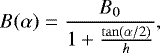 (3)
(3)
where B0 describes the amplitude of the opposition surge and h describes the width of the opposition peak. Although the inter-grain multiple scattering within the regolith on comet 67P/Churyumov-Gerasimenko was used to argue for the presence of a CBOE (Fornasier et al. 2015; Markkanen et al. 2018), the mechanism producing the opposition surge is still debated. Ryugu might be dominated by the shadow-hiding mechanism (SHOE) rather than the coherent backscatter contribution (CBOE) because of its dark nature. We apply this opposition effect term, since the shadow-hiding mechanism is considered to be the dominant source for the opposition effect (Hapke 1986, 2002, 2012). However, because the value of B0 may also include a coherent backscatter contribution, we cannot distinguish the contribution from these two mechanisms solely based on the value of B0. The single particle scattering function, P(α), is provided by a single-term Henyey-Greenstein function of the form
![Mathematical equation: \begin{equation*} P(\alpha)=\frac{(1-b^2)}{[1-2b\cos(\alpha)+b^2]^{3/2}}, \end{equation*}](/articles/aa/full_html/2020/07/aa37096-19/aa37096-19-eq6.png) (4)
(4)
where b describes the amplitude of the scattering peaks. A single term phase function is used since the data set does not capture the forward-scattering direction (α > 110°). The surface roughness, accounted for in the S(α, θ) term, is defined as the average slope over the resolution element of the detector (Hapke 1984). The derivation and mathematical expression for the surface roughness term can be found in Hapke (1984, 2012).
3.2 Disk-resolved model
The Hapke set of equations for describing disk-resolved reflectance,  , are given by:
![Mathematical equation: \begin{align*} \left(\frac{I}{F}\right)_R=&\,\frac{w}{4\pi}\frac{\mu_{0e}}{\mu_{0e}+\mu_e}\big\{P(\alpha)[1+B(\alpha)]]+[H(\mu_{0e})H(\mu_e)-1]\big\} \notag \\ &\cdot\, S(i,~e,~\alpha,~\bar{\theta}). \end{align*}](/articles/aa/full_html/2020/07/aa37096-19/aa37096-19-eq8.png) (5)
(5)
The surface roughness term,  , accounts for the large-scale roughness, and μ0e and μe are the modified cosines of the incident and emission angles, respectively, due to roughness. The H(x) terms are the Chandrasekhar H-functions, which are estimated using the expression:
 (6)
(6)
The mathematical expression of these terms, and their derivation can be found in Hapke (2012).
3.3 Modeling methods
The data were modeled in a step-wise approach. In the first step, only the disk-integrated data were modeled and only those bands whose disk-integrated data set includes both ground-based and ONC-T derived opposition measurements (b, v, Na, w, and x bands). There are no opposition measurements in the disk-resolved data used in this study. The data were modeled using a least-squares grid search that minimized the value of χ, defined by
 (7)
(7)
where N is the number of measurements, rmeasured is the measured reflectance, and rmodel is the model predicted reflectance. All parameters were varied simultaneously. Initial grid increment values were 0.01 for w, 0.1 for B0, 0.05 for h and b, and 2° for  . The initial results defined a narrower parameter space in which to search for final values. The final search was run with grid increment values of 0.001 for w, 0.01 for B0, 0.005 for h and b, and 1° for
  . The median value and variation for the opposition parameters were calculated across the five bands modeled. We found values for B0 and h of 0.98 and 0.075 with standard deviations of 0.021 and 0.008, respectively.
In the second step, the opposition parameter values for B0 and h were set to 0.98 and 0.075, respectively, for all bands. In this step all seven bands were modeled using both the disk-integrated and disk-resolved data sets. The model used a least-squares grid search, where separate χ values for the disk-integrated and disk-resolved data sets were calculated. The grid increment values were 0.001 for w and b, and 1° for  . The grid range was 0.02–0.07 for w, 0–0.4 for b, and 20°–40° for
  . These grid ranges were based on the results found in the first step. Maximum χ values for both the disk-integrated and disk-resolved modeling were provided, and all combinations of parameters over this grid and increment range with χ values lower than both disk-integrated and disk-resolved maximum values were stored and examined.
For each band, the resulting parameter sets were sorted, first according to the disk-integrated χ value, and then according to the disk-resolved χ value. The parameter sets with the top 20 lowest disk-integrated χ values were compared with the parameter sets with the top 20 lowest disk-resolved disk-integrated χ values. No identical parameter sets were found between these two groups of parameter sets for any of the bands, but parameter sets with the same w and  value were identified within each band. These solutions were selected as the “step-2” modeling result for that band.
In the third step, the median value for  (28° with a standard deviation of 6°) from the individual band results was calculated. The solutions from step-2 were then sorted as a function of χ value and those parameter sets with the median value of 28° were examined. The parameter set values for each band were examined independently in this step. The final result for each band was selected from this set of parameters based on minimizing the combined χ values. A third-order polynomial was fit to the w and b values as a function of band wavelength. This was done to remove any spurious spectral variations (e.g., Domingue et al. 2015).
Hapke parameter values for (162173) Ryugu.
3.4 Modeling results
The final parameter values are given in Table 4 for all bands. These parameters are the result of the simultaneous modeling of both the disk-integrated and disk-resolved data sets. The error bars stated for the opposition and roughness parameters are based on the standard deviations based on the results from step one and step two, respectively. These standard deviations are larger than the grid increments used in each step to find eachwavelength value. The error bars listed for the w and b were calculated based on the range of values found in step 3 over all wavelengths. If the range is smaller than the grid size, as is the case for the b values, then the final grid size is taken as the error estimate.
3.4.1 Disk-integrated data and model comparisons
Comparisons of the disk-integrated observations and measurements with the Hapke modeling results are shown in Fig. 7 for each band. The models show good agreement with the data. The two data set sources (ground-based and ONC-T) overlap within the error estimates for each data set, even within the opposition region. The Hapke model displayed corresponds to the values listed in Table 4. However, in the modeling process these solutions were not the only viable solutions to the disk-integrated data; they are the solutions that best describe the disk-integrated and disk-resolved data simultaneously.
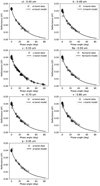 |
Fig. 7 Comparison of the disk-integrated observations of Ryugu (symbols) with the Hapke modeling (black line) results. The model curves shown correspond to the parameters listed in Table 4 from this study of Ryugu. |
3.4.2 Disk-resolved data and model comparisons
The disk-resolved data set and the modeling results were compared using ratios. The ratio of the measured reflectance to that of the model predicted reflectance was calculated. The resulting ratios were binned into four categories, and these are shown in Fig. 8: (1) ratios within 5% (values of 0.95–1.05), (2) ratios of 5–10% (values of 0.90–0.95 and 1.05–1.1), (3) ratios of 10–20% (values of 0.80–0.90 and 1.1–1.2), and (4) ratios >20% (values below 0.8 and above 1.2). As an example, the v-band reflectance values are plotted versus the model-predicted reflectance (Fig. 8). The majority of the disk-resolved data points fall into the <5% category for all bands, although the percentage of data points in this category decreases for the p band.
Figure 9 shows an example of the distribution of the four categories as a function of incidence and emission angle for the v band. The poorest fits (>20% category) are concentrated at higher values of incidence and emission angle. The disk-resolved data include shadows from boulders and craters, which can explain some of the poorly modeled measurements.
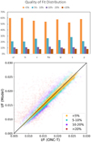 |
Fig. 8 Top: percentage of the disk-resolved data set for each band that is predicted by the Hapke model solution to within <5% (orange), to within 5–10% (light blue), to within 10–20% (purple), and to within >20% (red). Bottom: comparison of the ONC-T reflectance versus the model predicted reflectance, color-coded to match the percentage bins in the top graph, for the v band. The distribution and relationship is similar for the other bands. |
3.4.3 Geometric and bond albedo
The geometric or physical albedo, Ap, is the reflectance observed at zero phase angle relative to a Lambertian surface of the same cross-sectional area similarly illuminated and can be calculated directly from the Hapke set of equations (e.g., Hapke 1984, 2012). The phase integral, q, and the Bond albedo, AB, are related to the geometric albedo by the equation AB = Apq. The phase integral can be calculated from the equation
 (8)
(8)
where ϕ(α) is the radiancefactor. Using the Romberg method of integration, the phase integral was calculated for each band. The geometric albedo, phase integral, and Bond albedo for each band are shown in Table 5. The geometric albedo of 0.040 ± 0.005 is in the range of the geometric albedos of F- and C-types, namely 0.058 ± 0.023 and 0.061 ± 0.028, and is a little lower than those of other primitive B- and G-type asteroids, namely 0.113 ± 0.069 and 0.073 ± 0.018 (Usui et al. 2013).
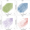 |
Fig. 9 Distribution of data over the incidence and emission angle space for each of the ratio categories for the v band. The points plotted in green are those that the model fits to <5% difference. The points plotted in blue are those that are fit to between 5 and 10%. The points plotted in purple are those that are fit to between 10 and 20%, and the points in red are those that fit to >20%. The data that are modeled to within 5% are evenly distributed across the angle space. As the model agreement with the data decreases, the distribution moves to the edges of the angle space. This corresponds to regions of higher incidence and emission angle values. |
Geometric, bond albedos, and phase integral for Ryugu.
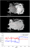 |
Fig. 10 Mosaic map made by the image hyb2_onc_20180831_112719 with phase angle of 40.4° and the image hyb2_onc_20180907_092745 with phase angle of 16.0°. Both images were acquired in the v band. Top: images without any photometric standardization. Middle: same mosaic after photometric standardization to (i, e, α) = (30°, 0°, 30°). Top and middle panels: scaled from 0 to 0.027. Bottom: reflectance profile along the red lines in the top and middle panels. |
4 Photometrically standardized albedo maps and mosaics
4.1 Evaluation of photometric standardization
One application of the photometric modeling is to provide standardization to a common viewing and illumination geometry. This is typically (i, e, α) = (30°, 0°, 30°), which corresponds to the viewing and illumination geometry of most laboratory reflectance measurements of planetary materials. A set of overlapping images were used to form a mosaic (Fig. 10) prior to standardization and then again after standardization. While the seam between images is still visible, the contrast between the images has been greatly reduced. Nevertheless, as an important example, we constructed a mosaic based on the 12 images acquired every 30° on the same day, 12 July 2018 (Fig. 11). This mosaic is a more realistic example of the types of mosaics used to construct a global map. We photometrically corrected the 12 images and removed the pixels which has incidence or emission values > 70°. All the images were overlaid without any smoothing at the borders. When the mosaic is made from the images taken on the same day, the seams between images are barely seen. This demonstrates that the photometric model provides a reasonable photometric standardization for constructing mosaics. A more in-depth disk-resolved study, which is beyond the scope of this work, could further reduce the contrast.
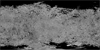 |
Fig. 11 Mosaic map made of 12 images for one rotation on 12 July 2018. Each image is photometrically standardized to (i, e, α) = (30°, 0°, 30°) without smoothing at the borders. The mosaic is scaled from 0.012 to 0.025. The border lines between the 12 images are barely seen. |
4.2 Albedo and color maps
Based on the Hapke modeling results shown in Sect. 3.4, we now examine the global albedo variations on Ryugu in the context of geologic features (Fig. 12). The full-disk images acquired from the home position, an altitude of ~20 km, were photometrically corrected and used to make a mosaic to form a v-band global albedo map (Fig. 13; other bands can be found in Appendix A). Here we defined the albedo as the reflectance factor with the illumination and viewing geometry of (i, e, α) = (30°, 0°, 30°). For the mosaic, we discarded the pixels with incidence or emission angles larger than 70°. The standard deviation in the albedo is ~10%. The east–west albedo dichotomy, brighter in the west area which includes Horai Fossa and Tokoyo Fossa (150°E–120°W), can be seen in all bands as was shown by Sugita et al. (2019). Moreover, this dichotomy is more prominent at the shorter wavelengths. The difference of albedo could reflect either a compositional and/or structural difference of regolith between east and west. For example, Michikami et al. (2019) reported the difference in the large boulder density distribution on east and west hemispheres. Therefore, the grain size of hemispheres could also be different. Furthermore, we found some dark regions are located in the large crater, such as Momotaro, Kibidango, Urashima, Brabo, and Cendrillon craters. The large craters might reveal dark interior materials.
We also constructed a spectral albedo ratio map by dividing the x-band albedo map by the v-band albedo map (Fig. 14). We can see color variation between correlated geological features. The blue color of the equatorial ridge, Tokoyo Fossa, and the south pole, as was reported by Sugita et al. (2019), is apparent. This spectral slope map shows that the northern hemisphere is more homogeneous in spectral slope than the southern hemisphere, while the south hemisphere displays variations more correlated to surface morphology, such as Tokoyo Fossa.
Twelve 1° × 1° regions wereselected, and the albedo values of the pixels in each region were averaged to create representative color spectra for each region, as shown in Fig. 15. Figure 15a shows the distribution of albedo and spectral slope for the global map with the same definition as Sugita et al. (2019). The spectral slope was calculated with a wavelength range of 0.48–0.86 μm. The spectral characteristics of TD1 and R3 are located on the global trend: bright blue to dark red. The reference spectrum (R3) was taken as an average of the region from [0°, 180°] to [30°N, 150°W] to clarify the spectral difference. To visualize the difference between regions, the regional spectra are divided by the reference spectrum (Fig. 15b right). We confirm the major correlation between the spectral slope and the albedo pointed out by Sugita et al. (2019). However, we observe minor places that display different trends. For example, the inside of Kibidango crater (K in Fig. 12) and Urashima crater (R1 in Fig. 12) have a relatively dark floor but the color is relatively blue. Another example is Otohime Saxum (O1 and O2 in Fig. 12), which is generally brighter than average but shows similar redness to the average, depending on the surface. The processes of brightening–darkening and bluing–reddening appears to be independent. Those exceptions suggest a more complicated history for Ryugu.
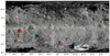 |
Fig. 12 Geologic map of Ryugu. Red points indicate the 12 regions of interest. |
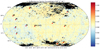 |
Fig. 13 v-band global albedo map of Ryugu. The albedo is defined by the reflectance factor with the illumination condition of (i, e, α) = (30°, 0°, 30°). Black patches are the place where the map does not have values due to high incidence and emission angles. |
5 Surface properties
5.1 Phase reddening properties
Spectral reddening (increase in spectral slope with increasing wavelength, in contrast to bluing, which is a decrease in spectral slope with increasing wavelength) with increasing solar phase angle is often observed on planetary surfaces, a phenomenon known as “phase reddening” (e.g., Gehrels et al. 1964). This effect has been observed on asteroids by both ground- and space-based instruments,and has been systematically investigated using laboratory measurements (Schröder et al. 2014a). Generally, phase reddening on opaque and dark objects is thought to be difficult to observe because it is related to multiple scattering and surface shadowing (Kaydash et al. 2010). However, recently the effect was observed on the dwarf planet Ceres (Ciarniello et al. 2017), the comet 67P/Churyumov-Gerasimenko (Fornasier et al. 2015), and the B-type asteroid Bennu (DellaGiustina et al. 2019). We also found weak phase reddening on Ryugu. The disk-integrated spectral slope between b- and x-bands, as a function of phase angle, is shown in Fig. 16. The strength of the phase reddening effect can be measured by the slope of the lines in Fig. 16: the larger the slope the greater the phase reddening. For Ryugu, we find a phase reddening slope of (2.0 ± 0.7) × 10−3μm−1 deg−1. The spectral slope variation of Ryugu is compared to two CM2 chondrites, MET 00639 and ALH 84040 (Hiroi et al. 2016b), suggesting slightly less phase reddening than those opaque and dark meteorites. The effect of grain size is shown to be small among those meteorites. However, the experiments by Schröder et al. (2014a) has shown that the microscopic roughness on the particle size scale and/or porosity could also affect the scattering property. Hence, the surface of boulders on Ryugu could be more complicated than those meteoritic samples on microscopic scale.
Phase reddening is thought to be associated with the multiple scattered component of reflected light (Adams 1967; Adams & Filice 1967; Schröder et al. 2014a). Thus, Ryugu’s regolith has a multiple scattering nature at longer wavelengths but the effect is very small. Because phase reddening is associated with multiple scattering within the regolith, the strength of phase reddening could be related to total reflectance. In Fig. 17, we investigated the relationship between the degree of phase reddening and albedo of several Solar System bodies, namely the Moon, Ceres, Vesta, Eros, Itokawa, 67P/Churyumov-Gerasimenko, and Bennu (Lane & Irvine 1973; Ciarniello et al. 2017; Schröder et al. 2014b; Clark et al. 2002; Tatsumi et al. 2018; Fornasier et al. 2015; DellaGiustina et al. 2019). It should be noted that only Eros was measured in the near-infrared wavelength range of 1.5–2.3 μm. Interestingly, Vesta does not show strong phase reddening, even if it is a very bright object. Eros shows much less phase reddening compared with Itokawa of similar albedo. Although 67P/Churyumov-Gerasimenko is known to be a very dark object, it exhibits significant phase reddening. Therefore, the relationship between the reflectance and degree of phase reddening is not very clear. Furthermore, this suggests that differences in grain structure and/or surface compaction condition may play a more significant role than reflectance (Schröder et al. 2014a). Moreover, Ryugu and Bennu have similar phase reddening properties, suggesting a similarity in the physical properties of Ryugu and Bennu, such as the microscopic roughness on the boulders and porosity.
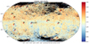 |
Fig. 14 Global albedo ratio map (Rx∕Rv). Black patches are the place where the map does not have values due to high incidence and emission angles. |
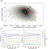 |
Fig. 15 (a) Global distribution of spectral slope (b-x) and reflectance factor. The white cross indicates the median value of the entire Ryugu surface. Yellow lines indicate the 65 and 95% distribution of all pixels. crosses indicate the 12 local spectral features. (b) Photometrically standardized spectra of the 12 regions shown in Figs. 12–14. The spectra on the right are divided by the spectrum of R3 to emphasize the variations. |
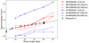 |
Fig. 16 Phase reddening trend of Ryugu and CM2 meteorites (MET 00639 and ALH 84040) of different grain size. Ryugu shows less phase reddening than the carbonaceous chondrites, although phase reddening is still apparent for this dark asteroid. |
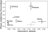 |
Fig. 17 Phase reddening on various Solar System airless bodies. The degree of phase reddening is measured by the variations in spectral slope with increasing phase angle. The Moon by Lane & Irvine (1973), Ceres by Ciarniello et al. (2017), Vesta by Schröder et al. (2014a), Eros by Clark et al. (2002), Itokawa by Tatsumi et al. (2018), 67P/Churyumov-Gerasimenko by Fornasier et al. (2015), and Bennu by DellaGiustina et al. (2019) are plotted with Ryugu (square). The effect on Eros was measured in the near-infrared, 1.5–2.3 μm, and other objects are measured in the visible wavelength range. |
5.2 Effect of the shape of the object
Generally asteroids are not perfect spheres, as demonstrated by the reports by the many spacecraft encounters with them to date. In the Hapke disk-integrated reflectance model, the equations assume that the shape of the observed body is a sphere. Therefore, there may be uncertainties introduced by this assumption, especially when applied to asteroids. To investigate this effect for Ryugu, we calculated the disk-integrated phase curve based on the shape model and compared it with the phase curve calculated in Eq. (2). To be more precise, the radiance factors for all illuminated polygons were calculated based on the realistic shape modeland the disk-resolved Hapke model to create a simulated image. The radiance factor was then integrated across all polygons to derive a disk-integrated radiance factor. We simulated phase curves at subspacecraft longitudes of 0°, 90°, 180°, and 270°. Figure 18 shows the comparison of the phase curves based on the simulated images using the shape model and Eq. (2).
The ratio between the shape model derived and the Hapke-equation-generated phase curves clearly demonstrates a difference, especially atthe larger phase angle values. The shape-model-simulated phase curve shows a larger opposition effect than the disk-integrated Hapke model equation which assumes a spherical shape. Thus, the parameters obtained based on the disk-integrated Hapke model may be overestimating the opposition parameter values for top-shaped asteroids. Moreover, even if the subspacecraft longitude is the same, depending on the sun-incidence direction, the disk-integrated reflectance can vary by a few percent due to the asymmetry in shadows from large boulders or longitudinal variations in shape. We need to exercise caution when applying disk-integrated Hapke model equations to irregularly shaped objects, which often applies to small bodies. This is a subject for further investigation using a more detailed disk-resolved model analysis. We note that the difference between the two phase curves is less than 6% for phase angles <40°, which corresponds to the conditions under which the ONC-T observations were taken.
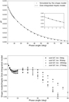 |
Fig. 18 Top:phase curves based on the shape model simulation (dot) and the disk-integrated Hapke model equation (dashed line). Bottom: ratio between the two phase curves; the radiance factor based on the shape model simulation is divided by the disk-integrated Hapke model as a function of incident solar light. |
5.3 Regolith properties from photometry
Photometricanalysis serves multiple purposes, from calibration validation to standardization for the production of mosaics and map products. However, models also can be used to bring some understanding of the physical properties of the surface. The Hapke model, derived from radiative transfer theories, links the values of the parameters to specific physical attributes of the scattering medium; in this case the surface regolith. While the validity of these correlations has been questioned and tested with mixed results (Shepard & Helfenstein 2007; Helfenstein & Shepard 2011; Souchon et al. 2011; Shkuratov et al. 2012), it helps place constraints on regolith characteristics especially when compared with other Solar System objects modeled with these same equations (Table 6).
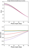 |
Fig. 19 Top: single particle phase function for each of the bands, corresponding to the amplitude parameter given in Table 4. All phase functions are backward scattering, with the amplitude of the back-scattering lobe being similar across these wavelengths. Bottom: ratio of the single particle scattering function of each band to the v-band single particle scattering function. The variation in the scattering function is below 5% over all phase angles, and below 2% over the phase angles observed by ONC-T. Phase reddening is seen in the spectral properties of Ryugu commensurate with the wavelength variations seen in the phase function. |
5.3.1 Single particle scattering function
Neither the disk-integrated or disk-resolved data sets sampled the forward scattering direction, and therefore only a single-term Henyey-Greenstein function was used to describe the single particle scattering function (P(α)). Figure 19 shows the single particle scattering function for each band. All bands display similar backward-scattering properties. This implies regolith grains with surface scatterers. The spectral variation in the single particle scattering function parameter, b, is essentially flat within the error estimates of the parameter value. This suggests that the structure of the regolith grains, at each of the filter band wavelengths, is very similar. In other words, the scattering centers that scatter light at 0.40 μm also scatter light at 0.95 μm, and vise versa. Even though the spectral variation in both b and single-scattering albedo are essentially flat, the subtle variations suggested in their values have opposite trends with wavelength. Phase reddening is seen in the spectral properties of Ryugu commensurate with the small wavelength variations seen in the phasefunction, which supports the hypothesis by Adams (1967) that multiple scattering plays role for phase reddening.
5.3.2 Surface roughness
Surface roughness is defined as the average surface tilt across all size ranges, from unresolved fine grains to the size of the detector footprint (Hapke 1984, 2012). For disk-integrated measurements, the effect of object shape (sometimes contained within the detector footprint size) factors into the estimation of this parameter. We have already shown that for the case of Ryugu the object shape can affect the phase curve reflectance by ~6%. Comparisons of the shapes of these three objects show that Ryugu is closest to a sphere (which is assumed by the model) and both Eros and Itokawa are elongated, irregularly-shaped ellipsoids. The comparison of the surface roughness parameter values with the contrasting surface images suggests that shape plays a significant role in the underlying value of the surface roughness parameter when examining disk-integrated data. Therefore, the disk-resolved data should be compared here. The Hapke parameter values displayed in Table 6 were derived with the inclusion of disk-resolved data sets.
Gaspra, an S-type asteroid similar in class to Itokawa, was examined by Helfenstein et al. (1994) and Domingue et al. (2016). The results from Helfenstein et al. (1994) predict a surface that is both darker and smoother than Itokawa. Domingue et al. (2016), in contrast, predict a surface that is brighter than that of Itokawa and smoother than those of all other objects shown in Table 6. However, Domingue et al. (2016) incorporated a two-term P(α), where the disk-resolved data they examined did not include measurements in the forward scattering direction. Using the same data set, with the opposition parameter values set to those of Helfenstein et al. (1994), we refit the Gaspra data using the same constraints as applied by this study to Ryugu. The resulting values (Table 6) indicate that Gaspra is darker than Itokawa but much brighter than Ryugu, as expected for an S-type compared to a C-type. Gaspra’s surface roughness in this updated analysis is also much smoother than that measured for Itokawa and Ryugu, and closer to that seen on Eros and Ida, which are both S-type.
The photometric analyses which include a disk-resolved dataset show a wide range of photometry roughness: 7.5–40° (Table 6). However, except for the largest value of Itokawa (Tatsumi et al. 2018) and the smallestvalue of Gaspra (Domingue et al. 2016), the photometric roughness scatters around 20–30°. Surprisingly, those values are also similar to the value for the Moon, although the surface of the Moon is covered by fine regolith. This might be because of roughness made by numerous craters on the Moon, while the numerous boulders account for the roughness on asteroids.
The surface roughness derived for Ryugu (28°) is smaller than that measured for Itokawa (40°; Tatsumi et al. 2018). However, images of these asteroids show that they each have unique surface regolith properties; Itokawa displays alternating regions of rocky coarse-grained regolith with areas of fine-grained dust, while the images of Ryugu show a surface that is rocky and coarse-grained, reminiscent of some of the regions on Itokawa. Itokawa has regions of ponded, fine-grained dust, which is noticeably absent on Ryugu. Nevertheless, Ryugu could possess unresolved fine grains on its surface uncovered by the touch-down operations (Morota et al. 2020).
Hapke parameter values for Ryugu compared with other asteroids and the Moon.
5.4 Comparison with meteorites
Using a photometric correction based on the modeling results in Sect. 3.4, we are able to compare Ryugu’s color spectrum with laboratory spectra of selected meteorite samples. The detection of a hydroxyl band absorption at 2.7 μm by NIRS3 suggests the existence of hydrated minerals on Ryugu (Kitazato et al. 2019). However, Ryugu is relatively dark compared with CM and CI class carbonaceous chondrites, which typically have reflectance of ~4–6% at the standard illumination and viewing angles (RELAB1). It is difficult to explain the dark and flat spectrum of Ryugu by comparisons with existing meteorites. Very few thermally metamorphosed meteorites of comparable spectral darkness and flatness are discussed in Sugita et al. (2019) and Kitazato et al. (2019). A comparison between the reflectance factor at i = 30°, e = 0°, and α = 30° (REFF(30, 0, 30)) of Ryugu and dark carbonaceous chondrites is shown in Fig. 20 (top). MET 00639 and Y-82162 are thermally metamorphosed carbonaceous chondrites and have the darkest and flattest spectra among naturally found meteorites. As shown in the figure, these meteorites are still more than 1.5 times brighter than Ryugu’s reflectance. Thus, it seems reasonable to consider that the material on Ryugu has different properties from the meteorite samples that we have found on Earth. If that is the case, the lower reflectance could be explained by additional effects, such as space weathering, higher thermal processing (Kitazato et al. 2019; Sugita et al. 2019), or different mineral composition. One possibility is that the surface of Ryugu contains a large amount of organic material: the more C present in the mineral composition, the lower the overall albedo becomes. The REFF(30, 0, 30) = 1.9% suggests C contents of more than 2 wt.% (Cloutis et al. 2012). The majority of the organic matter in carbonaceous chondrites are composed of insoluble organic material (IOM). We also compared Ryugu’s spectrum with the IOM spectra in CM chondrites, Murchison, and Y-86720 (Fig. 20 (bottom)). Insoluble organic material is usually darker than 3% and displays a flat slope in the visible wavelengths (Kaplan et al. 2019). Thus, a high IOM content may explain the darkness of Ryugu’s surface. At the same time, this is also consistent with the shallow 2.7-μm absorption seen in the NIRS3 spectra of Ryugu (Kitazato et al. 2019), since IOM spectra do not show strong absorptions.
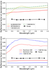 |
Fig. 20 Top: comparison of reflectance between Ryugu and carbonaceous chondrites (RELAB). Bottom: comparison of the reflectance between Ryugu and IOM of carbonaceous chondrites (Kaplan et al. 2019). |
6 Summary
Here we presented the spacecraft-based photometric observations of (162173) Ryugu acquired from the Hayabusa2 spacecraft ONC-T with seven color filters. In addition we presented new telescopic observations acquired with the Gemini-South telescope. Comparisons between the ONC-T measurements with both the Gemini-South telescopic observations and previous ground-based observationsdemonstrate that the ONC-T calibration is robust across all bands. One caveat that we encounter during these comparisons is that the quality of the ground-based spectra is very sensitive to the airmass during the observation run and aperture size of the telescope. We note that the phase curve derived from the ONC-T v-band images is in good agreement with the ground-based phase curve published by Ishiguro et al. (2014).
Ground-based observations show some spectral variability in the UV and some observations reveal a possible 0.7-μm band absorption. The color spectra observed by ONC-T show that Ryugu’s surface is dark and relatively homogenous, with no discernible spectral absorptions. Variations are seen in spectral slope and color ratio properties, which distinguish the equatorial ridge and polar regions from the mid-latitude regions, as was also seen by Sugita et al. (2019).
We modeled the photometric measurements of the asteroid Ryugu in all seven color band filters on ONC-T. We analyzed the dataset acquired from ~20 km away from the asteroid using both Hapke’s disk-integrated and disk-resolved models in order to make use of the ground-based data covering a wide range of phase angles and the spacecraft data covering a wide variety of incidence and emission angle conditions. The single scattering albedo derived for Ryugu is the smallest among other asteroids visited by spacecraft and modeled similarly. The geometric albedo and bond albedo were calculate based on our photometric model as 4.0 ± 0.5% and 1.4 ± 0.1%, respectively.
The roughness parameter derived for Ryugu is similar to that derived for many other asteroids. It is in the range of that estimated for Eros while being smoother than that estimated for Itokawa. However, it should be noted that the disk-integrated model assumes the planetary object is a sphere. There may be inherent error caused by the irregular shape of asteroids, which may affect the values of the roughness parameter. We demonstrate, for the case of Ryugu, the irregular top-shape introduces a ~2% difference in the derived disk-integrated reflectance in the opposition region (α < 10°) and a ~6% difference in the large phase angle (α > 40°) regions. Further analysis of the effect of shape is needed, but this is beyond the scope of this study.
The phenomenon of phase-reddening was observed on Ryugu. The degree of phase reddening ((2.0 ± 0.7) × 10−3 μm−1 deg−1) is comparable to that of the asteroid Bennu and laboratory spectral measurements of some thermally metamorphosed CM meteorites. Phase reddening is caused by multiply scattered light, common in fine-grained regolith. Thus, there could be weak multiple scattering on the surface of Ryugu suggesting the existence of very fine-grained (possible sub-micron-sized) material on the surface of this asteroid, perhaps coating the coarser grains, pebbles, and boulders visible on the surface.
Based on the albedo in this study, meteorite samples are still measurably brighter than Ryugu. Comparisons with IOM from CM meteorites show that this material could sufficiently darken and flatten carbonaceous chondrites without producing any spectral features and could therefore be a significant component of the Ryugu surface. Another possibility is that we do not yet have a sample of Ryugu in our meteorite collections. The ultimate answer awaits the return of the direct samples from the Ryugu surface collected by the Hayabusa2 spacecraft.
Acknowledgements
We gratefully acknowledge the work of the entire Hayabusa2 team to make these observations possible. Our ground-based spectra were taken by courtesy of Subaru Telescope, National Astronomical Observatory of Japan (NAOJ). We acknowledge the anonymous reviewer for careful reading and constructive comments to improve the manuscript. These data were obtained at the Gemini Observatory via the time-exchange program between Gemini and the Subaru Telescope. The Gemini Observatory is operated by the Association of Universities for Research in Astronomy, Inc. We are grateful to Dr. N. Levenson and Dr. F. Chaffee (Gemini Observatory) for their support andguidance in the observations by the Gemini-South telescope. In addition, we wish to thank Prof. H. Takami, Prof. N. Arimoto, and Prof. N. Ohashi (NAOJ) for negotiation and management of the telescope observing time allocation. We also express our gratitude to Dr. J. Durech for valuable comments, and to Dr. R. Binzel through SMASS, Dr. N. A. Moskovitz, Dr. D. Lazzaro, and Dr. D. Perna for kindly providing the spectra of Ryugu for comparison. This study is supported by the JSPS core-to-core program, “International Network of Planetary Science”, NASA’s Hayabusa2 Participating Scientist Program (grant number NNX16AL34G), and NASA’s Solar System Exploration Research Virtual Institute 2016 (SSERVI16) Cooperative Agreement (NNH16ZDA001N) for TREX (Toolbox for Research and Exploration). S.H. was supported by the Hypervelocity Impact Facility (former facility name: the Space Plasma Laboratory), ISAS, JAXA. T.H. was partially supported by NASA EW/PDART programs. D.K. was supported by Optical & Near-Infrared Astronomy Inter-University Cooperation Program, the MEXT of Japan. This research utilizes spectra acquired by R.E. Milliken with the NASA RELAB facility at Brown University. This study has made use of the USGS Integrated Software for Imagers and Spectrometers (ISIS).
Appendix A Albedo maps for all filters
Figures A.1–A.3 show the albedo maps defined by the reflectance factor at (i, e, α) = (30°, 0°, 30°) for all 7 band filters.
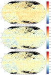 |
Fig. A.1 Albedo maps for the individual filter bands on the ONC-T (top: ul band, middle: b band, bottom: v band). |
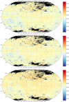 |
Fig. A.2 Albedo maps for the individual filter bands on the ONC-T (top: Na band, middle: w band, bottom: x band). |
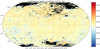 |
Fig. A.3 Albedo maps for the individual filter bands on the ONC-T (p band). |
Appendix B Data from RELAB
Table B.1 is the list of the sample IDs from the RELAB Database for ease in tracking the details of samples.
Samples used in this study from RELAB.
References
- Acton, C. H. 1996, Planet. Space Sci., 44, 65 [NASA ADS] [CrossRef] [Google Scholar]
- Adams, J. B. 1967, J. Geophys. Res., 72, 5717 [CrossRef] [Google Scholar]
- Adams, J. B., & Filice, A. L. 1967, J. Geophys. Res., 72, 5705 [CrossRef] [Google Scholar]
- Allen, C. W. 1973, Astrophysical Quantities (London: Athlone Press) [Google Scholar]
- Binzel, R. P., Harris, A. W., Bus, S. J., & Burbine, T. H. 2001, Icarus, 151, 139 [NASA ADS] [CrossRef] [Google Scholar]
- Bus, S. J., & Binzel, R. P. 2002, Icarus, 158, 146 [NASA ADS] [CrossRef] [Google Scholar]
- Ciarniello, M., Capaccioni, F., & Filacchione, G. 2014, Icarus, 237, 293 [NASA ADS] [CrossRef] [Google Scholar]
- Ciarniello, M., De Sanctis, M. C., Ammannito, E., et al. 2017, A&A, 598, A130 [NASA ADS] [CrossRef] [EDP Sciences] [Google Scholar]
- Clark, B. E., Veverka, J., Helfenstein, P., et al. 1999, Icarus, 140, 53 [NASA ADS] [CrossRef] [Google Scholar]
- Clark, B. E., Helfenstein, P., Bell, J. F., et al. 2002, Icarus, 155, 189 [NASA ADS] [CrossRef] [Google Scholar]
- Cloutis, E. A., Hudon, P., Hiroi, T., & Gaffey, M. J. 2012, Icarus, 220, 586 [NASA ADS] [CrossRef] [Google Scholar]
- DellaGiustina, D., Emery, J., Golish, D., et al. 2019, Nat. Astron., 3, 341 [Google Scholar]
- Domingue, D. L., Robinson, M., Carcich, B., et al. 2002, Icarus, 155, 205 [NASA ADS] [CrossRef] [Google Scholar]
- Domingue, D. L., Murchie, S. L., Denevi, B. W., Ernst, C. M., & Chabot, N. L. 2015, Icarus, 257, 477 [CrossRef] [Google Scholar]
- Domingue, D. L., Vilas, F., Choo, T., et al. 2016, Icarus, 280, 340 [CrossRef] [Google Scholar]
- Fornasier, S., Hasselmann, P. H., Barucci, M. A., et al. 2015, A&A, 583, A30 [NASA ADS] [CrossRef] [EDP Sciences] [Google Scholar]
- Gehrels, T., Coffeen, T., & Owings, D. 1964, AJ, 69, 826 [NASA ADS] [CrossRef] [Google Scholar]
- Gunderson, K., Thomas, N., & Whitby, J. A. 2006, Planet. Space Sci., 54, 1046 [CrossRef] [Google Scholar]
- Hapke, B. 1981, J. Geophys. Res., 86, 4571 [NASA ADS] [Google Scholar]
- Hapke, B. 1984, Icarus, 59, 41 [NASA ADS] [CrossRef] [Google Scholar]
- Hapke, B. 1986, Icarus, 67, 264 [NASA ADS] [CrossRef] [Google Scholar]
- Hapke, B. 2002, Icarus, 157, 523 [NASA ADS] [CrossRef] [Google Scholar]
- Hapke, B. 2012, Theory of Reflectance and Emittance Spectroscopy (Cambridge: Cambridge University Press) [Google Scholar]
- Hasselmann, P. H., Barucci, M. A., Fornasier, S., et al. 2017, MNRAS, 469, S550 [CrossRef] [Google Scholar]
- Helfenstein, P., & Shepard, M. K. 2011, Icarus, 215, 83 [NASA ADS] [CrossRef] [Google Scholar]
- Helfenstein, P., & Veverka, J. 1987, Icarus, 72, 342 [CrossRef] [Google Scholar]
- Helfenstein, P., Veverka, J., Thomas, P. C., et al. 1994, Icarus, 107, 37 [NASA ADS] [CrossRef] [Google Scholar]
- Helfenstein, P., Veverka, J., Thomas, P. C., et al. 1996, Icarus, 120, 48 [NASA ADS] [CrossRef] [Google Scholar]
- Hiroi, T., Kaiden, H., Imae, N., et al. 2016a, Lunar Planet. Sci. Conf., 1084 [Google Scholar]
- Hiroi, T., Miliken, R. M., & Pieters, C. M. 2016b, Hayabusa Symposium [Google Scholar]
- Hook, I. M., Jørgensen, I., Allington-Smith, J. R., et al. 2004, PASP, 116, 425 [NASA ADS] [CrossRef] [Google Scholar]
- Ishiguro, M., Kuroda, D., Hasegawa, S., et al. 2014, ApJ, 792, 74 [NASA ADS] [CrossRef] [Google Scholar]
- Kameda, S., Suzuki, H., Takamatsu, T., et al. 2017, Space Sci. Rev., 208, 17 [NASA ADS] [CrossRef] [Google Scholar]
- Kaplan, H. H., Milliken, R. E., Alexander, C. M. O., & Herd, C. D. K. 2019, Meteorit. Planet. Sci., 54, 1051 [CrossRef] [Google Scholar]
- Kaydash, V. G., Gerasimenko, S. Y., Shkuratov, Y. G., et al. 2010, Solar Syst. Res., 44, 267 [Google Scholar]
- Kitazato, K., Milliken, R. E., Iwata, T., et al. 2019, Science, 364, 272 [Google Scholar]
- Kuroda, D., Ishiguro, M., Takato, N., et al. 2014, PASJ, 66, 51 [NASA ADS] [CrossRef] [Google Scholar]
- Labarre, S., Ferrari, C., & Jacquemoud, S. 2017, Icarus, 290, 63 [CrossRef] [Google Scholar]
- Lane, A. P., & Irvine, W. M. 1973, AJ, 78, 267 [NASA ADS] [CrossRef] [Google Scholar]
- Lazzaro, D., Barucci, M. A., Perna, D., et al. 2013, A&A, 549, L2 [NASA ADS] [CrossRef] [EDP Sciences] [Google Scholar]
- Li, J., A’Hearn, M. F., & McFadden, L. A. 2004, Icarus, 172, 415 [NASA ADS] [CrossRef] [Google Scholar]
- Li, J.-Y., Le Corre, L., Schröder, S. E., et al. 2013, Icarus, 226, 1252 [NASA ADS] [CrossRef] [Google Scholar]
- Markkanen, J., Agarwal, J., Väisänen, T., Penttilä, A., & Muinonen, K. 2018, ApJ, 868, L16 [NASA ADS] [CrossRef] [Google Scholar]
- Masoumzadeh, N., & Boehnhardt, H. 2019, Icarus, 326, 1 [CrossRef] [Google Scholar]
- Michikami, T., Honda, C., Miyamoto, H., et al. 2019, Icarus, 331, 179 [CrossRef] [Google Scholar]
- Morota, T., Sugita, S., Cho, Y., et al. 2020, Science, 368, 654 [CrossRef] [Google Scholar]
- Moskovitz, N. A., Abe, S., Pan, K.-S., et al. 2013, Icarus, 224, 24 [NASA ADS] [CrossRef] [Google Scholar]
- Müller, T. G., Ďurech, J., Hasegawa, S., et al. 2011, A&A, 525, A145 [NASA ADS] [CrossRef] [EDP Sciences] [Google Scholar]
- Perna, D., Barucci, M. A., Ishiguro, M., et al. 2017, A&A, 599, L1 [NASA ADS] [CrossRef] [EDP Sciences] [Google Scholar]
- Sato, H., Robinson, M. S., Hapke, B., Denevi, B. W., & Boyd, A. K. 2014, J. Geophys. Res. Planets, 119, 1775 [NASA ADS] [CrossRef] [Google Scholar]
- Schröder, S. E., Grynko, Y., Pommerol, A., et al. 2014a, Icarus, 239, 201 [NASA ADS] [CrossRef] [Google Scholar]
- Schröder, S. E., Mottola, S., Matz, K. D., & Roatsch, T. 2014b, Icarus, 234, 99 [NASA ADS] [CrossRef] [Google Scholar]
- Schröder, S. E., Li, J.-Y., Rayman, M. D., et al. 2018, A&A, 620, A201 [NASA ADS] [CrossRef] [EDP Sciences] [Google Scholar]
- Shepard, M. K., & Helfenstein, P. 2007, J. Geophys. Res. Planets, 112, E03001 [NASA ADS] [CrossRef] [Google Scholar]
- Shepard, M. K., & Helfenstein, P. 2011, Icarus, 215, 526 [NASA ADS] [CrossRef] [Google Scholar]
- Shkuratov, Y., Kaydash, V., Korokhin, V., et al. 2012, J. Quant. Spectr. Rad. Transf., 113, 2431 [NASA ADS] [CrossRef] [Google Scholar]
- Souchon, A. L., Pinet, P. C., Chevrel, S. D., et al. 2011, Icarus, 215, 313 [NASA ADS] [CrossRef] [Google Scholar]
- Spjuth, S., Jorda, L., Lamy, P. L., Keller, H. U., & Li, J. Y. 2012, Icarus, 221, 1101 [NASA ADS] [CrossRef] [Google Scholar]
- Sugita, S., Honda, R., Morota, T., et al. 2019, Science, 364, 252 [Google Scholar]
- Suzuki, H., Yamada, M., Kouyama, T., et al. 2018, Icarus, 300, 341 [NASA ADS] [CrossRef] [Google Scholar]
- Tatsumi, E., Domingue, D., Hirata, N., et al. 2018, Icarus, 311, 175 [NASA ADS] [CrossRef] [Google Scholar]
- Tatsumi, E., Kouyama, T., Suzuki, H., et al. 2019a, Icarus, 325, 153 [Google Scholar]
- Tatsumi, E., Kameda, S., Moroi, K., et al. 2019b, Lunar Planet. Sci. Conf., 1745 [Google Scholar]
- Tholen, D. J. 1984, PhD thesis, University of Arizona, Tucson [Google Scholar]
- Usui, F., Kasuga, T., Hasegawa, S., et al. 2013, ApJ, 762, 56 [Google Scholar]
- Vilas, F. 2008, AJ, 135, 1101 [NASA ADS] [CrossRef] [Google Scholar]
- Vilas, F. 2012, AAS/Division for Planetary Sciences Meeting Abstracts, 44, 102.03 [Google Scholar]
- Vilas, F., & Gaffey, M. J. 1989, Science, 246, 790 [NASA ADS] [CrossRef] [PubMed] [Google Scholar]
- Watanabe, S., Hirabayashi, M., Hirata, N., et al. 2019, Science, 364, 268 [NASA ADS] [Google Scholar]
All Tables
All Figures
|
Fig. 1 Timing of our Ryugu observations using the Gemini-South telescope. (a) Apparent visual magnitude (AP-mag) of asteroid Ryugu provided by HORIZONS (https://ssd.jpl.nasa.gov/horizons.cgi). Our visible spectra were observed during the last observation opportunity (summer of 2012) before the launch of Hayabusa2 in December 2014. (b) Comparison of the rotational phases among our three observations. The black lines indicate the length of observations for these three nights. The blue lines indicate rotational phases that would have been observed at the respective observation times. |
| In the text | |
|
Fig. 2 Spectra of (162173) Ryugu obtained with the Gemini-South telescope on 24 and 26 June and 5 July, 2012. Spectra are normalized to unity at 0.55 μm and offsets between spectra are 0.2. |
| In the text | |
|
Fig. 3 Disk-integrated phase function for v band by ONC-T/Hayabusa2 (blue, red, green, black symbols) and by Ishiguro et al. (2014, gray symbols). |
| In the text | |
|
Fig. 4 Disk-average spectra of Ryugu with different phase angles. Error bars are 1-σ of different variation by rotational phase. |
| In the text | |
|
Fig. 5 Disk-average spectrum of Ryugu with taxonomy classification of Tholen (1984) and Bus & Binzel (2002). Hatched areas show the high and low values among those classes. Error bars were calculated based on the error in sensitivity calibration in Tatsumi et al. (2019a). |
| In the text | |
|
Fig. 6 Comparison between the 24 ground-based spectra (Binzel et al. 2001; Vilas 2008, 2012; Moskovitz et al. 2013; Lazzaro et al. 2013; Perna et al. 2017) and disk-average spectrum observed by ONC-T/Hayabusa2 at phase angles between 18.5° and 18.7°. All spectra are normalized to unity at 0.55 μm. The red points indicate the binned spectra by 0.02 μm and error bars are standard deviation inside of each bin. The ground-based observations are shown, ordered according to S/N values. |
| In the text | |
|
Fig. 7 Comparison of the disk-integrated observations of Ryugu (symbols) with the Hapke modeling (black line) results. The model curves shown correspond to the parameters listed in Table 4 from this study of Ryugu. |
| In the text | |
|
Fig. 8 Top: percentage of the disk-resolved data set for each band that is predicted by the Hapke model solution to within <5% (orange), to within 5–10% (light blue), to within 10–20% (purple), and to within >20% (red). Bottom: comparison of the ONC-T reflectance versus the model predicted reflectance, color-coded to match the percentage bins in the top graph, for the v band. The distribution and relationship is similar for the other bands. |
| In the text | |
|
Fig. 9 Distribution of data over the incidence and emission angle space for each of the ratio categories for the v band. The points plotted in green are those that the model fits to <5% difference. The points plotted in blue are those that are fit to between 5 and 10%. The points plotted in purple are those that are fit to between 10 and 20%, and the points in red are those that fit to >20%. The data that are modeled to within 5% are evenly distributed across the angle space. As the model agreement with the data decreases, the distribution moves to the edges of the angle space. This corresponds to regions of higher incidence and emission angle values. |
| In the text | |
|
Fig. 10 Mosaic map made by the image hyb2_onc_20180831_112719 with phase angle of 40.4° and the image hyb2_onc_20180907_092745 with phase angle of 16.0°. Both images were acquired in the v band. Top: images without any photometric standardization. Middle: same mosaic after photometric standardization to (i, e, α) = (30°, 0°, 30°). Top and middle panels: scaled from 0 to 0.027. Bottom: reflectance profile along the red lines in the top and middle panels. |
| In the text | |
|
Fig. 11 Mosaic map made of 12 images for one rotation on 12 July 2018. Each image is photometrically standardized to (i, e, α) = (30°, 0°, 30°) without smoothing at the borders. The mosaic is scaled from 0.012 to 0.025. The border lines between the 12 images are barely seen. |
| In the text | |
|
Fig. 12 Geologic map of Ryugu. Red points indicate the 12 regions of interest. |
| In the text | |
|
Fig. 13 v-band global albedo map of Ryugu. The albedo is defined by the reflectance factor with the illumination condition of (i, e, α) = (30°, 0°, 30°). Black patches are the place where the map does not have values due to high incidence and emission angles. |
| In the text | |
|
Fig. 14 Global albedo ratio map (Rx∕Rv). Black patches are the place where the map does not have values due to high incidence and emission angles. |
| In the text | |
|
Fig. 15 (a) Global distribution of spectral slope (b-x) and reflectance factor. The white cross indicates the median value of the entire Ryugu surface. Yellow lines indicate the 65 and 95% distribution of all pixels. crosses indicate the 12 local spectral features. (b) Photometrically standardized spectra of the 12 regions shown in Figs. 12–14. The spectra on the right are divided by the spectrum of R3 to emphasize the variations. |
| In the text | |
|
Fig. 16 Phase reddening trend of Ryugu and CM2 meteorites (MET 00639 and ALH 84040) of different grain size. Ryugu shows less phase reddening than the carbonaceous chondrites, although phase reddening is still apparent for this dark asteroid. |
| In the text | |
|
Fig. 17 Phase reddening on various Solar System airless bodies. The degree of phase reddening is measured by the variations in spectral slope with increasing phase angle. The Moon by Lane & Irvine (1973), Ceres by Ciarniello et al. (2017), Vesta by Schröder et al. (2014a), Eros by Clark et al. (2002), Itokawa by Tatsumi et al. (2018), 67P/Churyumov-Gerasimenko by Fornasier et al. (2015), and Bennu by DellaGiustina et al. (2019) are plotted with Ryugu (square). The effect on Eros was measured in the near-infrared, 1.5–2.3 μm, and other objects are measured in the visible wavelength range. |
| In the text | |
|
Fig. 18 Top:phase curves based on the shape model simulation (dot) and the disk-integrated Hapke model equation (dashed line). Bottom: ratio between the two phase curves; the radiance factor based on the shape model simulation is divided by the disk-integrated Hapke model as a function of incident solar light. |
| In the text | |
|
Fig. 19 Top: single particle phase function for each of the bands, corresponding to the amplitude parameter given in Table 4. All phase functions are backward scattering, with the amplitude of the back-scattering lobe being similar across these wavelengths. Bottom: ratio of the single particle scattering function of each band to the v-band single particle scattering function. The variation in the scattering function is below 5% over all phase angles, and below 2% over the phase angles observed by ONC-T. Phase reddening is seen in the spectral properties of Ryugu commensurate with the wavelength variations seen in the phase function. |
| In the text | |
|
Fig. 20 Top: comparison of reflectance between Ryugu and carbonaceous chondrites (RELAB). Bottom: comparison of the reflectance between Ryugu and IOM of carbonaceous chondrites (Kaplan et al. 2019). |
| In the text | |
|
Fig. A.1 Albedo maps for the individual filter bands on the ONC-T (top: ul band, middle: b band, bottom: v band). |
| In the text | |
|
Fig. A.2 Albedo maps for the individual filter bands on the ONC-T (top: Na band, middle: w band, bottom: x band). |
| In the text | |
|
Fig. A.3 Albedo maps for the individual filter bands on the ONC-T (p band). |
| In the text | |
Current usage metrics show cumulative count of Article Views (full-text article views including HTML views, PDF and ePub downloads, according to the available data) and Abstracts Views on Vision4Press platform.
Data correspond to usage on the plateform after 2015. The current usage metrics is available 48-96 hours after online publication and is updated daily on week days.
Initial download of the metrics may take a while.