| Issue |
A&A
Volume 639, July 2020
|
|
|---|---|---|
| Article Number | A39 | |
| Number of page(s) | 8 | |
| Section | Planets and planetary systems | |
| DOI | https://doi.org/10.1051/0004-6361/201935763 | |
| Published online | 03 July 2020 | |
Erosion of planetesimals by gas flow
1
Lund Observatory, Department of Astronomy and Theoretical Physics, Lund University,
Box 43,
22100
Lund,
Sweden
e-mail: This email address is being protected from spambots. You need JavaScript enabled to view it.
2
NORDITA,
Stockholm,
Roslagstullsbacken 23 106 91 Stockholm,
Sweden
3
Department of Physics, Gothenburg University,
41296
Gothenburg, Sweden
Received:
24
April
2019
Accepted:
15
May
2020
Abstract
The first stages of planet formation take place in protoplanetary disks that are largely made up of gas. Understanding how the gas affects planetesimals in the protoplanetary disk is therefore essential. In this paper, we discuss whether or not gas flow can erode planetesimals. We estimated how much shear stress is exerted onto the planetesimal surface by the gas as a function of disk and planetesimal properties. To determine whether erosion can take place, we compared this with previous measurements of the critical stress that a pebble-pile planetesimal can withstand before erosion begins. If erosion took place, we estimated the erosion time of the affected planetesimals. We also illustrated our estimates with two-dimensional numerical simulations of flows around planetesimals using the lattice Boltzmann method. We find that the wall shear stress can overcome the critical stress of planetesimals in an eccentric orbit within the innermost regions of the disk. The high eccentricities needed to reach erosive stresses could be the result of shepherding by migrating planets. We also find that if a planetesimal erodes, it does so on short timescales. For planetesimals residing outside of 1 au, we find that they are mainly safe from erosion, even in the case of highly eccentric orbits.
Key words: protoplanetary disks / methods: analytical / methods: numerical
© ESO 2020
1 Introduction
Planet formation begins with the collisional growth of micrometer-sized dust into millimeter-centimeter-sized pebbles. Through processes such as streaming instability, pebbles can then be concentrated into planetesimals with characteristic sizes of approximately 100 km (Youdin & Goodman 2005; Youdin & Johansen 2007; Johansen & Youdin 2007; Simon et al. 2016). Smaller planetesimals may form as a result of the fragmentation of such large planetesimals, boosting core formation by planetesimal accretion (D’Angelo et al. 2014). Other destructive interactions can take place in planetesimal-planetesimal collisions as well as in collisions between a planetesimal and any remaining pebbles; two outcomes of such collisions, among others, may be fragmentation (Wilkinson et al. 2008) and erosion (Güttler et al. 2010; Guilera et al. 2014; Bukhari Syed et al. 2017; Wahlberg Jansson et al. 2017). Since the initial stages of the planet formation process take place while the gas is still present in the disk, it is essential to also understand whether the interaction between the gas and planetesimals can also cause erosion.
Apart from a few previous works, the effect of gas on the erosion of disk solids has mostly been ignored. Paraskov et al. (2006) performed experiments and numerical calculations on the erosion of dust aggregates and found that solids on eccentric orbits are likely to be eroded in typical protoplanetary disk settings. Through parabolic flight experiments on the wind-induced erosion of a dust bed, Demirci et al. (2019) also show that within the inner protoplanetary disk the wall stress from the gas is enough to erode planetesimals. Through analytic calculations, Rozner et al. (2019) show that 10−104 meter solids are efficiently eroded by gas flow and Grishin et al. (2020) show that the resulting mono-sized pebbles provide the natural size cut-off for small pebbles.
In this paper, we study where erosion due to gas flow is significant in protoplanetary disks. We used an analytical model based on boundary-layer theory. We find the combination of the gas disk properties and planetesimal sizes that result in erosion in our model. For the planetesimal sizes where erosion is likely to be significant, we estimated the amount of time it takes to erode a given solid. We also built numerical models of the solid-gas interaction using the lattice Boltzmann method, which provided us with profiles of wall stress along the solid surface as a function of the Reynolds number.
In Sect. 2 we cover the theoretical aspect of the problem. In particular, we calculate the stress exerted by the gas onto planetesimals with varying sizes in typical protoplanetary disk settings. In Sect. 3 we present the results of the lattice Boltzmann method to perform numerical simulations of the gas flow around a solid obstacle. We summarize our result in Sect. 4 and discuss the lattice Boltzmann method in detail in Appendix A.
2 Boundary layer model
In order to understand how protoplanetary disk solids erode due to gas flow, we calculated the wall shear stress, τw, that is exerted by the gas onto the planetesimal surface. This stress is the tangential force per unit area exerted onto the planetesimal. Following Jäger et al. (2017), we assumed that if the wall shear stress exceeds a threshold value, τcr, the solid starts to erode. The rate of mass loss per unit area,  , which we also call the rate of erosion, is proportional to τw − τcr, that is,
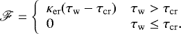 (1)
(1)
In Eq. (1) κer is a constant of proportionality that we call the erosion coefficient. Both the erosion coefficient and the critical stress depend on the materialproperties of the solid, for example, its composition and porosity. Equation (1) is purely empirical. This and similar erosion equations have been used for a long time – since the pioneering work by Shields (1936) – in studies of the erosion of river beds (see, e.g., Subhasish 2014 for an introduction). To find an estimate of the threshold stress can be quite a difficult task. For river beds a commonly used assumption is that the threshold stress is set by gravity and friction. For small planetesimals gravity is expected to play almost no role. The threshold stress should be set by surface forces.
For the erosion coefficient we used measurements from the experiments performed by Demirci et al. (2019). They studied the wind erosion of a bed of spherical glass beads in a setting that resembles protoplanetary disks moderately well. Near the erosion threshold, they measured a mass loss rate of about 0.6 kg m−2 s−1. This and the critical shear stress value set by the data from Demirci et al. (2019) (sum of gravity and cohesion) results in κer ~ 150 s m−1, given that τw − τcr ~ 4 × 10⁻⁴ at the threshold friction velocity. As seen in Eq. (1), the magnitude of κer is responsible for setting the efficiency of the rate of mass change. Thus, once experiments with conditions that resemble true protoplanetary disk settings are performed,  should be adjusted accordingly.
The wall shear stress exerted by the flow on the solid surface is defined as
 (2)
(2)
where μ = ρν is the dynamic viscosity, with ρ denoting the gas density and ν the kinematic viscosity. We chose our y axis along the wall normal direction and u is the stream-wise component of the velocity. We approximated Eq. (2) as
 (3)
(3)
where δ is the thickness of the boundary layer around a solid with size L, and U is the typical velocity of the mean flow. If the boundary layer is laminar (see, e.g., Landau & Lifshitz (1987), chapter IV), its thickness can be estimated as
 (4)
(4)
In terms of protoplanetary disk parameters, the wall shear stress defined in Eq. (3) becomes
 (5)
(5)
where the density and the kinematic viscosity of the disk are set according to the adopted protoplanetary disk model (e.g., the minimum mass solar nebula, Hayashi 1981). The parameter U in this case is defined as the speed difference between the gas and the planetesimal, in other words, the headwind. For a planetesimal on an eccentric orbit, the headwind is not a constant but depends on the details of the planetesimal’s orbit. For a planetesimal, in a orbit with zero inclination at perihelion, the headwind is given by (Adachi et al. 1976)
 (6)
(6)
where η is the proportionalto the ratio of the squares of the mean thermal speed of the gas molecules and the Keplerian speed (Adachi et al. 1976). The value of η is estimated to be approximately 10−3. In Eq. (6),  is the Keplerian speed at a distance, r, from the central star with solar mass, M⊙.
The critical shear stress that a protoplanetary disk solid can withstand is determined by the strength of its surface layer. Skorov & Blum (2012) model the tensile strength of ice-free outer layers of comet nuclei given that they are agglomerates of dust aggregates. They conclude that the effective tensile strength of such a layer is
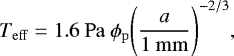 (7)
(7)
where ϕp = 1 − P is the volume filling factor and a is the size of the aggregate. Baer et al. (2011) present the bulk porosity, P, of more than 50 main-belt asteroids as P ~ 0.1−0.7. Taking P = 0.4 as the average porosity, the effective tensile strength of a 1 mm dust aggregate is τcr = 0.96 Pa. We also compared the wall shear stress exerted by the gas to the critical shear stress determined by experiments presented in Paraskov et al. (2006). They performed experiments on centimeter-sized dust aggregates in a wind tunnel, where they studied the effect of gas flow on the aggregates, which consisted of about 500 μm dust granules. They found that in the case of a planetesimal on an eccentric orbit, τcr = 25 Pa.
Figure 1 shows the comparison between the wall shear stress from our boundary layer model and the critical shear stress from Paraskov et al. (2006) (marked with black dashed line) and Skorov & Blum (2012) (marked with orange dashed line) as a function of orbital distance. The eccentricity of the planetesimal orbit is taken as e = 0.1 in a minimum mass solar nebula model. The four solid curves in Fig. 1 correspond to different planetesimal sizes. Overall, τw increases with decreasing planetesimal size and with decreasing distance from the central star. Thus, erosion due to gas flow is likely to be most efficient in the inner protoplanetary disk.
The wall shear stress as defined in Eq. (5) is a function of the disk density and viscosity and the Keplerian velocity, which are all functions of the radial coordinate of the planetesimal, r. The velocity in addition also depends on the eccentricity of the orbit as stated in Eq. (6). Finally, τw depends on the size of the planetesimal itself. Based on Eqs. (5) and (6) we expect that erosion due to the wall shear stress exerted by the gas flow increases with orbital eccentricity and is most effective in the inner disk. To understand the relationship between the wall shear stress and r, e, and L we can turn to Fig. 2, where we show our model predictions for the wall shear stress as a function of orbital eccentricity and planetesimal size at r = 0.2 au, r = 1 au, and r = 5 au. The black curves correspond to τw = 0.96 Pa, which is thecritical shear stress from Skorov & Blum (2012). According to Fig. 2a, at r = 0.2 au most planetesimal sizes seem to experience erosion. Once the realistic eccentricity of the planetesimal with the given size is taken into account as well, we can conclude that large planetesimals (~ 100 km) are only likely to experience erosion in the inner regions of the disk, given the presence of a large planet to excite the eccentricities. Planets tend to migrate as they interact with the gas disk (Walsh et al. 2012; Morbidelli et al. 2012; Batygin & Laughlin 2015; Ida et al. 2018; Johansen et al. 2019). As they migrate, they can shepherd planetesimals in the inner disk and excite their eccentricities (Tanaka & Ida 1999). Smaller planetesimals are likely to be eroded by the gas flow as well, as shown in Fig. 2a. Figure 2b shows that beyond r = 1 au planetesimals are not expected to be eroded, since the wall shear stress only exceeds τcr where the planetesimals are likely too small to acquire high enough eccentricities in realistic protoplanetary disk settings. Already at a distance of 5 au, it is highly unlikely that any planetesimal would be eroded by gas flow, as shown in Fig. 2c. Consequently, the ideal regime for erosion due to gas flow is in the inner r ≈ 1 au of protoplanetary disks. Erosion due to gas flow is most significant for small planetesimals of ~ 100 m and large planetesimals of ~100 km on eccentric orbits.
It is non-trivial to estimate the time it takes for a planetesimal to erode away because as the planetesimal erodes, its size changes and so does the flow around it. As a result, the wall shear stress changes as well. Here, we present only an estimate that is based on the wall stress calculated from the initial size of the planetesimal such that the erosion time is
 (8)
(8)
where the total planetesimal mass is
 (9)
(9)
where ρ∙ is the material density of the solid and the volume of the planetesimal is  . The area of the planetesimal in Eq. (8) is
  . We take ρ∙ = 5.4 × 10² kg m−3, which is the approximate bulk density of 67P/Churyumov-Gerasimenko (Pätzold et al. 2019). The erosion time is defined only in regions where τw >τcr. Given that a planetesimalis within the regime where erosion due to gas flow is possible, the erosion is very fast, as shown in Fig. 3. The figure also shows that ter is a strong function of planetesimal size, such that it decreases with decreasing L.
As shown in Fig. 3, the erosion happens on a short timescale, whereas the radial drift timescale is on the order of ~102−104 yr in the inner disk (Youdin 2010). As a result, if the planetesimals come into gravitational contact with a migrating planet and thus acquire excited eccentricities, they erode away almost instantaneously, without experiencing radial drift.
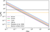 |
Fig. 1 Scaling of the wall shear stress exerted on planetesimals with varying sizes as a function of orbital distance, r. Here, we assume an orbital eccentricity of e = 0.1. The black dashed line marks the 25 Pa limit for erosion given by Paraskov et al. (2006). The orange dashed line marks the 0.96 Pa limit of the tensile strength of dust layers on comets given by Skorov & Blum (2012). The solid curves with varying colors correspond to varying planetesimal sizes. |
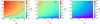 |
Fig. 2 Wall shear stress as a function of planetesimal size, L, and orbital eccentricity, e, at an orbital distance of (a) r = 0.2 au, (b) r = 1 au, and (c) r = 5 au. The black solid curve corresponds to τw = 0.96 Pa, which we take as the critical shear stress that a planetesimal can withstand before it begins to erode (Skorov & Blum 2012). |
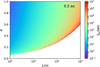 |
Fig. 3 Erosion time as a function of planetesimal size, L, and orbital eccentricity, e, at an orbital distance of r = 0.2 au. The erosion time is defined only, where τw > τcr. |
3 Numerical model
To model the stress on the planetesimal we have developed a new code using the lattice Boltzmann method, which is described in Appendix A in detail. Usually, most codes used in astrophysics do not allow us to solve for flows with arbitrary boundaries, which is necessary in this problem. The immersed boundary method has been used in Mitra et al. (2013) to calculate flows around spherically shaped planetesimals facing a headwind. However, during erosion the shape of the body changes dynamically, thus we used the lattice Boltzmann method. Here, we did not implement erosion in our code and did not solve the flow for a dynamically changing boundary, but calculated the wall shear stress for just the initial shape and size of the planetesimal. We still used the lattice Boltzmann method, since it has the possibility of extending our calculations to the dynamicallychanging case.
We built a two-dimensional code to simulate the flow around a planetesimal and measured the wall shear stress exerted onto its surface. In order to understand how the flow properties influence the outcome, we then compared the results as a function of the Reynolds number. This is a non-dimensional number and is a measure of the balance between inertial and viscous forces defined as
 (10)
(10)
Through the Reynolds number of the numerical model (see Eq. (A.7)), one can scale the numerical setup to physical protoplanetary disk values. The Reynolds number can be written as
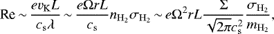 (11)
(11)
where λ is the mean free path of the gas, Ω is the Keplerian angular frequency, and  is the surface density of the disk. In Eq. (11), the sound speed is denoted with cs and its value is set according to the minumum mass solar nebula (MMSN) model at a distance of r = 1au. The number density of hydrogen molecules is
  . For the collisional cross section of the hydrogen molecule, we used
  from Chapman & Cowling (1970). The mass of the molecule is
  . In the minimum mass solar nebula Re thus scales as
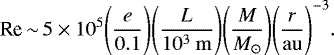 (12)
(12)
The relationship of Re to planetesimal size and eccentricity at an orbital distance of r = 0.2 au is shown in Fig. 4. The black curve corresponds to the limit set by the critical wall shear stress (τcr = 0.96 Pa), below which gas erosion does not occur. Thus, Fig. 4 shows that the relevant Reynolds numbers for the erosion of planetesimals by the gas flow at r = 0.2 au are Re ~ 106−1011.
The time for the flow to pass the planetesimal is
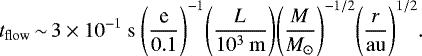 (13)
(13)
We compared this to the typical rotation timescale of 67P/Churyumov-Gerasimenko of trot ~ 12 h (Jorda et al. 2016). Given that tflow < trot, the flow adapts to the instantaneous direction of the planetesimal. In the case where tflow > trot, the flow sees the planetesimal shape in an average sense. We note, however, that rotation is not considered here.
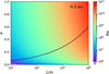 |
Fig. 4 Reynolds number as a function of planetesimal size and eccentricity at an orbital distance of r = 0.2 au according to the minimum mass solar nebula model. The black curve corresponds to the critical shear stress limit of τcr = 0.96 Pa (Skorov & Blum 2012). |
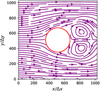 |
Fig. 5 Streamlines of the flow around a circle (marked with red) given Re ≈ 128. The streamlines separate in front of the obstacle and two eddies appear behind it. |
3.1 Flow structure
The numerical model provides us with a flow profile around the solid obstacle. Given a small Reynolds number, the flow that develops around an obstacle is laminar (Landau & Lifshitz 1987). A laminar flow results in smooth, parallel streamlines that separate around the given obstacle. As the Reynolds number increases the laminar flow becomes unstable, such as the one presented in Fig. 5, where Re ≈ 128 and two eddies form behind the solid.
3.2 Wall shear stress profile around solid surface
We studied how the flow affects different parts of the solid by looking at the profile of the wall shear stress along the surface. As the mass flux presented in Eq. (1) is proportional to the wall shear stress, this gives a direct indication of which parts of the obstacle will erode more efficiently. We plot the wall shear stress normalized by the mean stress,  , along the surface in Fig. 6. The figure shows that the parts of the solid that are expected to be eroded the least are near the stagnation points of the flow. The wall shear stress is highest near the top of the circle, after which it decreases slightly again at the very top. As expected from the symmetry of the model setup, the wall shear stress profile is symmetric along the horizontal bisector that passes through the midpoint of the circle.
To understand how changing the Reynolds number of the flow affects the erosion rate, we compared  for varying values of Re around the surface in Fig. 7. We see that the pattern of the exerted stress changes somewhat as a function of the Reynolds number. The maxima of the curves increase when comparing low Reynolds number flows (Re < 1) to the ones with Re > 1. The maxima saturate to similar wall shear stress values as instabilities set in (Re > 1).
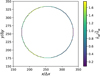 |
Fig. 6 Wall shear stress over the surface of the obstacle normalized by the mean wall shear stress along the whole surface. The Reynolds number of the flow is Re ~ 8. As the wall shear stress is proportional to the mass flux, the erosion is most efficient near the top and bottom of the obstacle (marked with red) and least efficient near the stagnation points of the flow (marked with purple). |
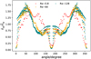 |
Fig. 7 Wall shear stress along the surface of the obstacle as a function of angle. The angle of 0° corresponds to the stagnation point on the upstream side of the surface in Fig 6. The different colors correspond to different Reynolds numbers. The pattern of erosion as a result of the wall shear stress exerted by the gas is not a significant function of the Re. |
4 Summary and discussion
Our results show that planetesimals can erode by the action of the gas disk in the inner parts of protoplanetary disks, r ≲1 au. As giant planets migrate through the disk and shepherd the planetesimals in front of them, they leave them with excited eccentricities (Tanaka & Ida 1999), which facilitates their erosion. We find that gas erosion affects small planetesimals of ~ 100 m on orbits with eccentricities larger than 0.1 and large planetesimals of ~ 100 km on orbits with eccentricities above 0.5. Outside of r ~1 au, most disk solids are not largely affected by gas erosion. We also find that if gas erosion is effective, the erosion time of a given planetesimal is short.
To illustrate the erosion profile along planetesimals, we developed a numerical code using the lattice Boltzmann method (see Appendix A). From the numerical model we found that, based on the distribution of the wall shear stress along the solid surface, erosion is fastest near the top and bottom of the obstacle and slowest near the stagnation points of the flow. We also found that the Reynolds number of the flow does not significantly alter the pattern of erosion along the surface within the range of Reynolds numbers considered here. Our results lead us to predict that no planetesimal will be found in eccentric orbits in the inner parts of a protoplanetary disk.
This conclusion is subject to some caveats that we discuss below. Firstly, we estimated the wall shear stress via the ratio of the headwind velocity and the thickness of the boundary layer. The latter can have quite complex behavior. As the planetesimal faces the headwind, there must be a stagnation point at the front. If we assume that the boundary layer remains laminar, its thickness grows as the square root of the distance from the stagnation point measured along the direction of the flow along the planetesimal surface. Let us use the symbol ξ for this coordinate, that is,  . However, this dependence is not true close to the stagnation point. Here, the boundary layer thickness becomes a non-zero constant set by the flow at the stagnation point (Landau & Lifshitz 1987). As ξ increases, we surmise that the wall shear stress increases, reaches a maximum value, and then decreases roughly as
  , since δ increases in the same manner. This qualitative behavior of the wall shear stress is seen in Fig. 6. However, this picture does not hold for large planetesimals or for large Reynolds numbers. In the case of large planetesimals the boundary layer becomes unstable at the critical value of ξ. This critical value depends on the mean flow, U, and possibly other details, such as the curvature of the planetesimal surface, how smooth or rough the surface is, and upon the porosity of the material. For ξ larger than this critical value there is no known simple dependence of the boundary layer thickness on ξ. For very large ξ and thus large planetesimals, the boundary layer can be turbulent and the empirical relation δ ~ ξ1∕5 may hold. To estimate whether a planetesimal erodes at all we need to determine the maximum wall shear stress. As this estimation is challenging, we chose to use the laminar boundary layer and use the minimum value of the stress thus obtained as our estimate of the stress. Hence, we may grossly underestimate the wall shear stress, particularly for large planetesimals. Thus, it is possible that in reality the planetesimals erode even faster than we estimate here.
Secondly, as the planetesimal erodes, its shape and size changes. This in turn changes the wall shear stress. We have ignored this effect in our estimates. A more accurate estimate, following Ristroph et al. (2012), will be presented in a future work. However, as we have explained before, for large planetesimals we expect our estimate to provide a lower limit to the wall shear stress. As the size of the planetesimal decreases, our description of the boundary layer as a laminar one becomes more accurate, thus we expect that the inclusion of the dynamical boundary change will make the planetesimal erode even faster than estimated here.
Thirdly, we note that for planetesimals on circular orbits, the headwind is in general too small to cause any erosion. However, as η (the ratio of the thermal speed of gas molecules and the Keplerian speed) is very small, even a small eccentricity will give rise to erosion. We expect that planetesimals in the inner disks can survive only if they are on nearly circular orbits. In the case of a large eccentricity, two additional effects need to be considered, which are not present in our model. One is that the variation of gas density in the orbit can be quite large. The density is highest where the speed is largest hence we expect erosion will increase further. The second new effect is that the headwind can become so large that it becomes supersonic. As far as we know, there is no easy way to estimate the wall stress in such a situation. The lattice Boltzmann method we used in this paper will not work for supersonic flows either. Numerical methods following Rusanov (1976) can be used. Developing numerical methods for supersonic erosion should be a high priority for future studies of planetesimal erosion.
Finally, the estimate of the threshold stress has a large amount of uncertainty. Our estimates are based on experiments performed with pebble piles but planetesimals are also expected to have significant amounts of ice in them. The presence of ice may increase the threshold stress manyfold. Furthermore, in a large pile the material inside may become more compact by sintering. Thus the threshold stress for the inner material may be significantly larger than that of the outer layer. Thus, we may find that the erosion is very effective in removing the surface layer of planetesimals but becomes less effective as the inner layers are exposed. We expect our results will encourage further work on this topic
Acknowledgements
We thank the anonymous referee for their input and comments that helped improve the manuscript. N.S. would like to thank H. Capelo for inspiring discussions. N.S. was funded by the “Bottlenecks for particle growth in turbulent aerosols” grant from the Knut and Alice Wallenberg Foundation (2014.0048). A.J. thanks the Swedish Research Council (grant2014-5775), the Knut and Alice Wallenberg Foundation (grants 2012.0150,2014.0017), and the European Research Council (ERC Consolidator Grant724687-PLANETESYS) for research support.
Appendix A Lattice Boltzmann method
The lattice Boltzmann method relies on kinetic theory (Sukop & Thorne 2007). The fluid is described as particles that exchange momentum and energy through advection and collision. These particles are described by the probability distribution function, f(x, v, t) = f, which represents the population of particles with position, x, and velocity, v, at time, t. The system is then described with the Boltzmann equation, which, given that there is no external force acting on the system, can be written as
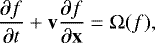 (A.1)
(A.1)
where Ω(f) is the collision operator.
In the lattice Boltzmann method the continuous Boltzmann equation is discretized in both velocity and physical space. The lattice Boltzmann equation is then solved on a lattice, where the particles are restricted to movement along discrete directions between the nearest and next-nearest neighbors of a two-dimensional Cartesian lattice. The particle velocities are thus described by ea, where a are the direction indexes. As shown in Fig. A.1, we used the two-dimensional D2Q9 model, such that a = 1, 2,..., 9, and e5 represents a particle at rest (marked as the gray node on Fig. A.1).
The advection term in Eq. (A.1) is implemented as a streaming process, where the probability distributions propagate along the discrete velocity vectors. The collision term in Eq. (A.1) is most widely approximated with the Bathnagar-Gross-Krook collision operator (Bhatnagar et al. 1954). Thus, the lattice Boltzmann equation becomes
![Mathematical equation: \begin{equation*} f_a(\mathbf{x}+\mathbf{e}_a \Delta t, t+\Delta{t})=f_a(\mathbf{x},t)-\frac{\Big[f_a(\mathbf{x},t)-f^{\rm{eq}}_a(\mathbf{x},t)\Big]}{\tau},\end{equation*}](/articles/aa/full_html/2020/07/aa35763-19/aa35763-19-eq28.png) (A.2)
(A.2)
where fa(x, t) describes the directional distribution function. According to Eq. (A.2), particles fa (x, t) move to neighboring lattice nodes at time t + Δt with velocity ea, which represents the streaming part of the method. The collision of the particles is described by the second term on the right-hand side of Eq. (A.2), where τ is the relaxation time and  is the equilibrium distribution function given by
![Mathematical equation: \begin{equation*} f^{\rm{eq}}_a(\mathbf{x},t)=w_a \rho \Bigg[1+3\frac{\mathbf{e}_a \cdot \mathbf{u}}{c^2}+\frac{9}{2} \frac{(\mathbf{e}_a \cdot \mathbf{u}^2)}{c^4}-\frac{3}{2}\frac{\mathbf{u}^2}{c^2} \Bigg].\end{equation*}](/articles/aa/full_html/2020/07/aa35763-19/aa35763-19-eq30.png) (A.3)
(A.3)
In Eq. (A.3), wa represents the weights associated with each direction, such that
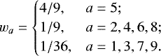 (A.4)
(A.4)
In Eq. (A.3), ρ = ρ(x, t) and u = u(x, t) are the macroscopic fluid density and velocity, and c is the lattice speed.
The macroscopic fluid density and velocity are calculated using the weighted sums of the probability distribution function’s moments, such that the macroscopic fluid density becomes
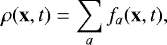 (A.5)
(A.5)
and the macroscopic fluid velocity is
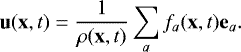 (A.6)
(A.6)
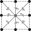 |
Fig. A.1 Illustration of the streaming step in the lattice Boltzmann method. The particle distributions are streamed into the central lattice node from neighboring nodes with lattice velocities of ea. |
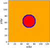 |
Fig. A.2 Example model set-up, where the solid obstacle (red) is surrounded by the gas flow (orange). In between the two lie the surface points (blue), such that the solid points do not directly come into contact with the flow. |
A.1 Initial and boundary conditions
The initial conditions of the numerical model are set via the parameters that make up the Reynolds number, which is defined as
 (A.7)
(A.7)
in terms of the parameters of the lattice Boltzmann model. In Eq. (A.7) u′ is the velocity of the fluid in units of the lattice speed, c. In our model the lattice speed is set to c = 1. The planetesimal size, L′, is measured in units of the cell size, which we set as Δx = 1. The lattice viscosity is proportional to the relaxation time, such that
 (A.8)
(A.8)
Figure A.2 shows an example set-up, where the solid obstacle is a circle (marked with red), which is surrounded with surface nodes (marked with blue). The surface nodes act as the boundary between the obstacle and the fluid nodes (marked with orange). The lattice Boltzmann equation presented in Eq. (A.2) is solved on the fluid but not on the solid nodes. The dynamics on the surface nodes are determined by the no-slip boundary condition.
The no-slip boundary condition ensures that particles hitting the surface nodes are bounced back, such that there is no flow into the solid obstacle. The boundary conditions of the model are periodic in the vertical direction such that the distribution functions leaving at the top of the simulation box are the same as the ones at the bottom. Thus, the boundary condition in the vertical direction is such that
 (A.9)
(A.9)
 (A.10)
where y0 and yNy+1 are virtual lattice nodes that act as ghost zones around the simulation domain. In the horizontal direction we apply the Dirichlet boundary condition, such that we set the velocity to a constant value at the inlet and the outlet of the simulation domain.
A.2 Wall shear stress
The wall shear stress is calculated using the shear stress tensor defined as
 (A.11)
In the lattice Boltzmann method this is calculated as
 (A.12)
where  is the non-equilibrium part of the distribution function (Jäger et al. 2017). The force felt by the surface is then the shear tensor multiplied by the surface normal vector,
  , such that
 (A.13)
Finally, the wall shear stress is the magnitude of the force such that
 (A.14)
References
- Adachi, I., Hayashi, C., & Nakazawa, K. 1976, Prog. Theor. Phys., 56, 1756 [NASA ADS] [CrossRef] [Google Scholar]
- Baer, J., Chesley, S. R., & Matson, R. D. 2011, AJ, 141, 143 [NASA ADS] [CrossRef] [Google Scholar]
- Batygin, K., & Laughlin, G. 2015, Proc. Natl. Acad. Sci., 112, 4214 [Google Scholar]
- Bhatnagar, P. L., Gross, E. P., & Krook, M. 1954, Phys. Rev., 94, 511 [CrossRef] [Google Scholar]
- Bukhari Syed, M., Blum, J., Wahlberg Jansson, K., & Johansen, A. 2017, ApJ, 834, 145 [NASA ADS] [CrossRef] [Google Scholar]
- Chapman, S., & Cowling, T. G. 1970, The Mathematical Theory of Non-uniform Gases. An Account of the Kinetic Theory of Viscosity, Thermal Conduction and Diffusion in Gases (Cambridge: Cambridge University Press) [Google Scholar]
- D’Angelo, G., Weidenschilling, S. J., Lissauer, J. J., & Bodenheimer, P. 2014, Icarus, 241, 298 [NASA ADS] [CrossRef] [Google Scholar]
- Demirci, T., Kruss, M., Teiser, J., et al. 2019, MNRAS [Google Scholar]
- Grishin, E., Rozner, M., & Perets, H. B. 2020, ArXiv e-prints [arXiv:2004.03600] [Google Scholar]
- Guilera, O. M., de Elía, G. C., Brunini, A., & Santamaría, P. J. 2014, A&A, 565, A96 [NASA ADS] [CrossRef] [EDP Sciences] [Google Scholar]
- Güttler, C., Blum, J., Zsom, A., Ormel, C. W., & Dullemond, C. P. 2010, A&A, 513, A56 [NASA ADS] [CrossRef] [EDP Sciences] [Google Scholar]
- Hayashi, C. 1981, IAU Symp., 93, 113 [Google Scholar]
- Ida, S., Tanaka, H., Johansen, A., Kanagawa, K. D., & Tanigawa, T. 2018, ApJ, 864, 77 [NASA ADS] [CrossRef] [Google Scholar]
- Jäger, R., Mendoza, M., & Herrmann, H. J. 2017, Phys. Rev. E, 95, 013110 [CrossRef] [Google Scholar]
- Johansen, A., & Youdin, A. 2007, ApJ, 662, 627 [NASA ADS] [CrossRef] [Google Scholar]
- Johansen, A., Ida, S., & Brasser, R. 2019, A&A, 622, A202 [NASA ADS] [CrossRef] [EDP Sciences] [Google Scholar]
- Jorda, L., Gaskell, R., Capanna, C., et al. 2016, Icarus, 277, 257 [NASA ADS] [CrossRef] [Google Scholar]
- Landau, L., & Lifshitz, E. 1987, Fluid Mechanics (Oxford, UK: Pergamon Press) [Google Scholar]
- Mitra, D., Wettlaufer, J. S., & Brandenburg, A. 2013, ApJ, 773, 120 [NASA ADS] [CrossRef] [Google Scholar]
- Morbidelli, A., Lunine, J. I., O’Brien, D. P., Raymond, S. N., & Walsh, K. J. 2012, Ann. Rev. Earth Planet. Sci., 40, 251 [NASA ADS] [CrossRef] [Google Scholar]
- Paraskov, G. B., Wurm, G., & Krauss, O. 2006, ApJ, 648, 1219 [NASA ADS] [CrossRef] [Google Scholar]
- Pätzold, M., Andert, T. P., Hahn, M., et al. 2019, MNRAS, 483, 2337 [NASA ADS] [CrossRef] [Google Scholar]
- Ristroph, L., Moore, M. N. J., Childress, S., Shelley, M. J., & Zhang, J. 2012, Proc. Natl. Acad. Sci., 109, 19606 [CrossRef] [Google Scholar]
- Rozner, M., Grishin, E., & Perets, H. B. 2019, ArXiv e-prints [arXiv:1910.02941] [Google Scholar]
- Rusanov, V. V. 1976, Ann. Rev. Fluid Mech., 8, 377 [CrossRef] [Google Scholar]
- Shields, I. 1936, PhD thesis, University of Berlin, Berlin, Germany [Google Scholar]
- Simon, J. B., Armitage, P. J., Li, R., & Youdin, A. N. 2016, ApJ, 822, 55 [NASA ADS] [CrossRef] [Google Scholar]
- Skorov, Y., & Blum, J. 2012, Icarus, 221, 1 [NASA ADS] [CrossRef] [Google Scholar]
- Subhasish, D. 2014, Fluvial Hydrodynamics (Berlin: Springer) [Google Scholar]
- Sukop, M. C., & Thorne, T. D. J. 2007, Lattice Boltzmann Modeling (Berlin: Springer) [Google Scholar]
- Tanaka, H., & Ida, S. 1999, Icarus, 139, 350 [NASA ADS] [CrossRef] [Google Scholar]
- Wahlberg Jansson, K., Johansen, A., Bukhari Syed, M., & Blum, J. 2017, ApJ, 835, 109 [NASA ADS] [CrossRef] [Google Scholar]
- Walsh, K. J., Morbidelli, A., Raymond, S. N., O’Brien, D. P., & Mandell, A. M. 2012, Meteorit. Planet. Sci., 47, 1941 [NASA ADS] [CrossRef] [Google Scholar]
- Wilkinson, M., Mehlig, B., & Uski, V. 2008, ApJS, 176, 484 [CrossRef] [Google Scholar]
- Youdin, A. N. 2010, EAS Pub. Ser., 41, 187 [Google Scholar]
- Youdin, A. N., & Goodman, J. 2005, ApJ, 620, 459 [NASA ADS] [CrossRef] [Google Scholar]
- Youdin, A., & Johansen, A. 2007, ApJ, 662, 613 [NASA ADS] [CrossRef] [Google Scholar]
All Figures
|
Fig. 1 Scaling of the wall shear stress exerted on planetesimals with varying sizes as a function of orbital distance, r. Here, we assume an orbital eccentricity of e = 0.1. The black dashed line marks the 25 Pa limit for erosion given by Paraskov et al. (2006). The orange dashed line marks the 0.96 Pa limit of the tensile strength of dust layers on comets given by Skorov & Blum (2012). The solid curves with varying colors correspond to varying planetesimal sizes. |
| In the text | |
|
Fig. 2 Wall shear stress as a function of planetesimal size, L, and orbital eccentricity, e, at an orbital distance of (a) r = 0.2 au, (b) r = 1 au, and (c) r = 5 au. The black solid curve corresponds to τw = 0.96 Pa, which we take as the critical shear stress that a planetesimal can withstand before it begins to erode (Skorov & Blum 2012). |
| In the text | |
|
Fig. 3 Erosion time as a function of planetesimal size, L, and orbital eccentricity, e, at an orbital distance of r = 0.2 au. The erosion time is defined only, where τw > τcr. |
| In the text | |
|
Fig. 4 Reynolds number as a function of planetesimal size and eccentricity at an orbital distance of r = 0.2 au according to the minimum mass solar nebula model. The black curve corresponds to the critical shear stress limit of τcr = 0.96 Pa (Skorov & Blum 2012). |
| In the text | |
|
Fig. 5 Streamlines of the flow around a circle (marked with red) given Re ≈ 128. The streamlines separate in front of the obstacle and two eddies appear behind it. |
| In the text | |
|
Fig. 6 Wall shear stress over the surface of the obstacle normalized by the mean wall shear stress along the whole surface. The Reynolds number of the flow is Re ~ 8. As the wall shear stress is proportional to the mass flux, the erosion is most efficient near the top and bottom of the obstacle (marked with red) and least efficient near the stagnation points of the flow (marked with purple). |
| In the text | |
|
Fig. 7 Wall shear stress along the surface of the obstacle as a function of angle. The angle of 0° corresponds to the stagnation point on the upstream side of the surface in Fig 6. The different colors correspond to different Reynolds numbers. The pattern of erosion as a result of the wall shear stress exerted by the gas is not a significant function of the Re. |
| In the text | |
|
Fig. A.1 Illustration of the streaming step in the lattice Boltzmann method. The particle distributions are streamed into the central lattice node from neighboring nodes with lattice velocities of ea. |
| In the text | |
|
Fig. A.2 Example model set-up, where the solid obstacle (red) is surrounded by the gas flow (orange). In between the two lie the surface points (blue), such that the solid points do not directly come into contact with the flow. |
| In the text | |
Current usage metrics show cumulative count of Article Views (full-text article views including HTML views, PDF and ePub downloads, according to the available data) and Abstracts Views on Vision4Press platform.
Data correspond to usage on the plateform after 2015. The current usage metrics is available 48-96 hours after online publication and is updated daily on week days.
Initial download of the metrics may take a while.